7-1964
Design and operation of a flat linear induction
pump
Delwyn Donald Bluhm
Iowa State UniversityR. W. Fisher
Iowa State UniversityJ. W. Nilsson
Iowa State UniversityFollow this and additional works at:
http://lib.dr.iastate.edu/ameslab_isreports
Part of the
Engineering Commons
This Report is brought to you for free and open access by the Ames Laboratory at Iowa State University Digital Repository. It has been accepted for inclusion in Ames Laboratory Technical Reports by an authorized administrator of Iowa State University Digital Repository. For more information, please [email protected].
Recommended Citation
Bluhm, Delwyn Donald; Fisher, R. W.; and Nilsson, J. W., "Design and operation of a flat linear induction pump" (1964).Ames Laboratory Technical Reports. 92.
Abstract
A five pole, one slot per phase, full pitch, twelve coil, wye connected, three phase linear induction pump has been designed for operation with 400 C sodium. The design incorporated a graded winding in order to reduce the net pulsating component of the magnetic flux density wave and a pump duct using copper side bars. The small laboratory-size pump was designed in two steps: stator design and winding design. First, the stator and core dimensions were established on the basis of maximum pressure development and maximum power at the design flow and slip. Maximum pressure output was a requirement of the intended pump application. The condition of maximum power output was used in order to provide a good pump efficiency. Second, the parameters for the induction pump equivalent circuit were determined for several winding methods. The winding method which offered 3920 ampere turns per phase (equivalent to a flow rate of 4. 88 gpm, a pressure of 60 psi, a line voltage of 250 volts, and a wave length of 21.2 cm as calculated in the first step) was selected. The theoretical performance characteristics of the flat induction pump were computed using the equivalent circuit parameters for a winding with 60 turns per coil. The measurement of developed pressure (0 to 42. 13 psi), sodium flow rate (0 to 9. 93 gpm), and power input (0 to 103. 9 watts) after installation of the pump in an operational sodium circulating loop provided an experimental determination of the pump performance characteristic. In addition, the effect of pump duct temperature on sodium flow rate and a differential transformer system used to locate the sodium level in manometer columns were briefly discussed .
Disciplines Engineering
IOWA STATE UNIVERSITY
DESIGN AND OPERATION OF A FLAT LINEAR INDUCTION PUMP
by
Delwyn Donald Bluhm, R. W. Fisher and J. W. Nilsson
PHYSICAL SCIENCES REflJ>ING R
~
&~~~ ~£[ID®~&1J®~W
RESEARCH AND
DEVELOPMENT
REPORT
Engineering and Equipment (UC-38} TID-4500, September 1, 1964
UNITED STATES ATOMIC ENERGY COMMISSION Research and Development Report
DESIGN AND OPERATION OF A FLAT LINEAR INDUCTION PUMP
by
Delwyn Donald Bluhm, R. W. Fisher and J. W. Nilsson
July, 1964
Ames Laboratory at
Iowa State University of Science and Technology F. H. Spedding, Director
IS-991
This report is distributed according to the category Engineering and Equipment (UC-38), as listed in TID-4500, September 1, 1964.
r - - - -
LEGAL NOTICE---.
This report was prepared as an account of Government sponsored work. Neither the United States, nor the Commission, nor any person acting on behalf of the Commission:
A. Makes any warranty or representation, expressed or implied, with respect to the accuracy, completeness, or usefulness of the information contained in this report, or that the use of any information, apparatus, method, or process disclosed in this report may not infringe privately owned rights; or
B. Assumes any liabilities with respect to the use of, or for damages resulting from the use of any information, apparatus, method, or process disclosed in this report.
As used in the above, "person acting on behalf of the Commission" includes any employee or contractor of the Commission, or employee of such contractor, to the extent that such employee or contractor of the Commission, or employee of such contractor prepares, disseminates, or provides access to, any information pursuant to his employment or contract with the Commission, or his employment with such contractor.
Printed in USA. Price
$
3. 00 Available from theTABLE OF CONTENTS
LIST OF SYMBOLS
Optimum Stator Structure
Winding Design
ABSTRACT
I. INTRODUCTION
II. ELECTROMAGNETIC PUMPS
III. REVIEW OF DESIGN THEORY
A. Optimum Stator Structure
B. Windings
IV. THEORETICAL DESIGN OF PUMP
A. Optimum Stator Structure
B. Windings
C. Theoretical Performance Characteristics
V. INVESTIGATIONS
A. Equipment
B. Experimental Procedure
VI. EXPERIMENTAL RESULTS
VII. CONCLUSIONS AND SUMMARY
VIII. LITERATURE CITED
IX. APPENDIX
A B ~ d f F Fa Fm g H I
Im, im
LIST OF SYMBOLS
Optimum Stator Structure
rms ampere conductors per unit length
instantaneous gap flux density
amplitude of gap flux density
equivalent pump duct diameter
frequency
instantaneous value of armature mmf wave
amplitude of armature mmf wave
magnetizing component of F
total magnetic gap
head loss
rms stator phase current
amplitude and instantaneous yalues of magnetizing component
of Is per unit length
amplitude and instantaneous values of liquid current wave,
power component of Is per unit length
amplitude and instantaneous values of total equivalent stator
surface current density per unit length
amplitude and instantaneous values of duct current wave,
power component of Is per unit length
kinematic viscosity of fluid
winding distribution factor
winding factor, kd kp
K pump parameter,
pump parameter to give maximum value of zh and z0 at constant
s and X
pump parameter for optimum design, s0
=
se, zh=
z0 maximum,X constant
1 distance measured in direction of induced currents
n number of poles
NPH total series turns per phase
p average pressure developed per unit length of pump
(p)actual actual average pressure developed, (xp - P£)
P£ hydraulic friction loss (experimentally determined)
P power loss in the liquid metal per unit length
Pi input power to liquid metal
P0 ideal power output in the liquid metal per unit length
(P0)actual actual power output in the liquid metal (total)
power loss in the pump duct wall per unit length
q number of phases
Q total flow
Reynolds number
resistance of liquid parallel to Ir
combined resistance of top and bottom pump duct walls
slip for maximum efficiency at constant X
slip for maximum pressure at constant Is' X and K
slip for maximum developed power at constant X and K
t internal thickness of pump duct parallel to magnetic field
thickness of pump duct wall
v velocity of liquid metal in pump duct
relative velocity between liquid and synchronous field
w
X
X
velocity of magnetic field
internal width of pump duct parallel to current flow
distance measured in direction of flow
P
2 twwall loss parameter, Pw
t
head utilization factor, non-dimensional part of formula for p
maximum value of zh with variable K
maximum value of zh with variable s
output utilization factor, non-dimensional part of formula
z0k maximum value of z0 with variable K
z08 maximum value of z0 with variable s
a,~ phase angles
(~)actual actual operating efficiency
~e electrical efficiency
~em maximum electrical efficiency
~h hydraulic efficiency
8
p
CT
cos
8
E~
f
g
I
internal phase angle between Is and Ir + Iw
viscosity of liquid metal
wavelength or double pole pitch
resistivity of liquid
resistivity of pump duct wall material
density of liquid metal
internal power factor
Winding Design
area of gap orthogonal to magnetic field (i.e., L wB) square
inches
cross sectional area of conductor, square inches
cross sectional area of copper side bars, square inches
circuits in parallel
depth of slot occupied by conductors, inches
conductor free depth of slot, inches
equivalent diameter of copper side bars (i.e.
-1-)
.,.
inchesline to line voltage, volts
phase to neutral voltage, volts
frequency, cps
total magnetic gap, inches
rms stator phase current, amperes
magnetizing current, amperes
winding distribution factor
L
(MLC)
n
s
t
t w
w
length of magnetic field, pump or pump duct over wound region,
inches
mean length of conductor, inches
number of poles
primary conductors in series per phase
number of phases
primary resistance per phase, ohms
equivalent resistance of fluid per phase referred to stator,
ohms
equivalent resistance of duct walls per phase referred to
stator, ohms
slip,
number of stator slots containing copper
total slots in iron
internal thickness of pump duct parallel to magnetic field,
inches
thickness of pump duct wall, inches
internal width of pump duct parallel to current flow, inches
effective field width (i.e. iron width x stacking factor),
·inches
slot width, inches
primary leakage reactance, ohms at f
magnetizing reactance, ohms at f
p
~u
Pw
resistivity of liquid, microhm inches
resistivity of copper, microhm inches
DESIGN AND OPERATION OF A FLAT LINEAR INDUCTION PUMP···
Delwyn D. Bluhm, R. W. Fisher and J. W. Nilsson
ABSTRACT
A five pole, one slot per phase, full pitch, twelve coil, wye
connected, three phase linear induction pump has been designed for
operation with 400 C sodium. The design incorporated a graded
wind-ing in order to reduce the net pulsating component of the magnetic flux
density wave and a pump duct using copper side bars. The small
laboratory-size pump was designed in two steps: stator design and
winding design. First, the stator and core dimensions were
establish-ed on the basis of maximum pressure development and maximum power
at the design flow and slip. Maximum pressure output was a
require-ment of the intended pump application. The condition of maximum
power output was used in order to provide a good pump efficiency.
Second, the parameters for the induction pump equivalent circuit were
determined for several winding methods. The winding method which
offered 3920 ampere turns per phase (equivalent to a flow rate of 4. 88
gpm, a pressure of 60 psi, a line voltage of 250 volts, and a wave
length of 21.2 em as calculated in the first step) was selected. The
theoretical performance characteristics of the flat induction pump
were computed using the equivalent circuit parameters for a winding
with 60 turns per coil. The measurement of developed pressure (0 to
42. 13 psi), sodium flow rate (0 to 9. 93 gpm), and power input (0 to 103. 9
watts) after installation of the pump in an operational sodium circulating
loop provided an experimental determination of the pump performance
characteristic. In addition, the effect of pump duct temperature on
sodium flow rate and a differential transformer system used to locate
the sodium level in manometer columns were briefly discussed .
.,_
.,.
I. INTRODUCTION
Devices which rely on the force that is produced whenever a current
carrying solid conductor is imbedded in a magnetic field are well known
to today's engineers and scientists. Not so well known are the two
groups of devices in which the current is carried either in a conductive
gas or a conductive liquid.
An example of a device using a conducting gas is the MHD
(Magneto-hydrodynamic) generator (1). The gas is made conductive by partial
ionization and is forced to cut a magnetic field. Electrodes
perpendic-ular to the field draw off the induced currents. Electromagnetic pumps
and flowmeters are two very good examples of devices.using conductive
liquids. The conductive liquids are usually molten metals at high
temperatures. The electromagnetic pump provides the current and ~gnetic
field in the conductive liquid. The resulting force which causes the
liquid to be pumped is the useful output. The electromagnetic flowmeter
operates on the same principal as the MHD generator except
that the conductive mediums are different. The induced EMF at the
electrodes is proportional to the rate of flow of the conductive liquid.
This work deals primarily with electromagnetic pumps. These pumps
have become increasingly important in the last few years due to the
expanded use of molten metals as heat-transfer mediums for nuclear power
plants. Pumps developed for this purpose are normally very large. For
example,an A. C. linear induction pump for Argonne's Experimental Breeder
Reactor II (2) has a capacity of 5,000 gpm of 700 F sodium at 40 psi
less frequently used to circulate liquid metals and alloys in corrosion test loops (3) and to feed aluminum to a die-casting machine (4).
The object of this work was to design and determine the performance
II. ELECTROMAGNETIC PUMPS
In 1907 Northrup (5) developed a hydrostatic pressure of several
inches of water via the interaction of a 600 ampere current and a
magnetic field in mercury. He postulated that this effect could be
utilized in an ammeter for measuring large currents.
The movement of a liquid metal by using a sliding and rotating
magnetic field was proposed by Chubb (6) in 1915. Bainbridge (7) tested
an alternating current conduction pump in 1926. Einstein and Szilard
proposed an annular linear induction pump for use with alkali metals in
1928. Several working models of this pump rated at about 2 kw were
operated with mercury and liquid alloys of sodium and potassium. The
design equations for this type of pump using liquid bismuth were
pre-sented in a report by Feld and Szilard (8) in 1942.
The flat linear induction pump is only one of many types of
electro-magnetic pumps for liquid metals. The principal of operation is the same
for all electromagnetic pumps. It is the source of the current and
magnetic field that changes. Electromagnetic pumps can be divided in
two main categories; they are the conduction pumps and the induction
pumps.
Conduction pumps may be operated either on alternating or direct
current. Either type pump may be identified by the electrodes, brazed
to the pump duct wall, which supply the current from an external source
to the liquid metal. Conduction pumps have one primary advantage over
the other electromagnetic pumps; they can be used to pump even the
high density, and high viscosity. The current flowing through the liquid
metal may be made as large as is necessary to overcome the effects of the
heavy metals. The biggest disadvantage of these pumps is the requirement
of extremely large currents, usually several thousand amperes at volta~es
of one or two volts.
A direct current conduction pump can be operated either with a
permanent magnet or an electromagnet to produce the magnetic field. The
disadvantage of the awkward excitation requirements, as mentioned earlier,
is partially overcome by the use of a relatively efficient homopolar
generator with liquid metal brushes. The use of conventional rectifiers
is not recommended for the larger pumps since they are inefficient,
bulky, and expensive. Another requirement (and not always a disadvantage)
for satisfactory operation of a direct current pump is the wetting of
the duct wall by the liquid metal. The performance characteristics of
the direct current conduction pump are excellent as the pump is applicable
in systems requiTing wide variations in power, pressure, and flow. In
efficiency too, the direct current pump is unsurpassed by the other types
of electromagnetic pumps.
In order to avoid the use of a homopolar generator, an alternating
current conduction pump with its associated step-down transformer is
sometimes used. The immediate problems encountered with this pump are:
lamination of magnetic circuit to reduce eddy-currents and iron losses
and thereby improve the normally low efficiency; physically laTger pump;
poor power factor; and noisy operation. The alternating current
with size at a constant frequency. However, larger pumps may be built
if the frequency is sufficiently lowered. Normally, the reliable
step-down transformer is employed near or is part of ~he pump,while alternate
sources of supply may be located remotely.
The second category of electromagnetic pumps, the induction pumps,
always have alternating current induced in the molten metal by a
travel-ing or pulsattravel-ing magnetic field. These pumps are normally, with one
exception, used only with the typical light metals with higher
conduc-tivities so that the induced currents will be sufficiently large. A
classification of the most common types is:
Single-phase annular
Polyphase helical
Polyphase flat linear
Polyphase annular linear
Rotating magnet
The single-phase annular induction pump is similar to a transformer
with stationary primary winding but a moveable secondary winding. The
liquid metal acts as the secondary winding, and it is pumped by the
interaction of radial primary magnetic field in the annular gap and
the circulating induced current in the liquid. This pump is generally
used only for small pumping requirements because of its inherent low
efficiency and poor power factor. For larger pumping capacities the
The polyphase helical induction pump employs a rotating magnetic
field produced in the same manner as a squirrel cage induction motor.
The squirrel cage is replaced by a cylindrical liquid metal duct in an
increased air gap surrounding a "blocked" cylindrical iron core. Helical
guide vanes are placed in the duct to impart axial motion to the liquid
which is rotating from the action of the rotating magnetic field produced
by the three-phase stator winding. The function of end rings is now
served partially by the liquid and partially by two copper rings,silver
soldered to the duct at each end of the core. A helical induction pump
of this type normally is used in applications requiring high pressure
and low flow.
The most popular polyphase induction pump is the flat linear type.
The resulting linear fluid motion is an improvement upon the helical
induc-tion pump when large flows are required. The flat linear inducinduc-tion pump
is most easily described as a helical pump which has been cut open axially
along one side and finally straightened into a flat rectangular shape.
The duct is now located between two axially laminated structures. To
' improve pump performance,copper side bars are usually added to each side
of the duct; they function as end rings in a conventional induction motor.
The traveling field is produced by the polyphase multipole stator
wind-ings located on either one or both of the laminated iron structures. The
losses in this pump may be substantially reduced by grading the magnetic
field in the end sections. Grading allows the magnetic field to gradually
increase from near zero at the ends to the uniform value over the fully
An important feature of this pump is the possible removal of the stator
structures and windings without disturbing the liquid metal system.
The annular linear pump (or Einstein-Szilard pump) can be thought of
as being formed from the flat linear type by bending the latter into a
cylindrical shape. The radially laminated, cylindrical core, now on the
inside of an annular duct, has no windings. The windings,which are
pan-cake-like coils,are located in the circular slots of the stator
surround-ing the pump duct. Copper side bars are not needed since the induced
currents in the liquid metal flow in circular closed-loop paths. The
reduction of end effects by field grading is essential for good
perform-ance. As compared to the flat linear pump, the annular pump offers lower
hydraulic loss, stronger and less complicated construction, lower heat
loss, easier field grading, higher leakage reactance, and a more
compli-cated winding removal procedure.
Rotating field induction pumps induce an alternating current in the
liquid metal through the use of mechanically rotated permanent magnets
or electromagnets. All of the polyphase induction pumps with rotating
magnetic fields can be modified to form a rotating magnet pump. The
usual arrangement is to use rotating magnets for pumps with loop or helix
pump ducts. Copper side bars are required. This type of induction pump
has several-advantages over the other types, such as a stronger available
field providing the possibility of pumping high-resistivity metals, the
near unity power factor operation of induction motors, self-cooled magnets,
good efficiency and variable pole pitch. The drawbacks include the use of
The linear induction type of electromagnetic pump was selected since
it has proven its ability to operate continuously at temperatures near
1000 C for as long as 5000 hours (9). This is a very important capability
when a pump is to be used in corrosion test loops for circulating metals
with high melting points. This selection was also made since it was hoped
that this work would justify the use of small flat linear induction pumps
in laboratory applications where the pumping requirements are normally
very small. In the literature the flat linear induction pump was most
commonly employed at large flows for high efficiency while the single
phase induction pump and the rotating magnet induction pump were the two
types most frequently designed for laboratory use. The efficiencies of
these two types of pumps are generally low at the low flow rates where
they are employed. The use of the flat linear induction pump offers the
advantage of a simpler fabrication technique than with the single phase
induction pump; however, the efficiency is slightly less. It offers
several advantages over the rotating magnet pump,such as the elimination
of moving parts and a simplified pump duct removal procedure. Even
though the efficiency of a flat linear induction pump decreases at low
flow, proper design of the pump should yield an acceptable .efficiency.
In fact,this efficiency should compare favorably with the efficiencies
of the other small pumps under similar operating conditions.
Normally, the efficiency of linear induction pumps for corrosion
loops is unimportant. However, efficiency is a consideration in test
loops which are to be operated under design conditions of flow rate and
with an efficiency of 0.12% (9) or lower could cause the heat input to
the molten metal to be excessive. This fact necessitated the design of
a more efficient flat linear induction pump at a preselected flow rate.
The pump was designed specifically for a working fluid of sodium. Sodium
is one of the best metals for use with linear induction pumps since it is
a typical light metal with low resistivity, low density, and low
viscosity.
The availability of an operational sodium loop provided a means of
III. REVIEW OF DESIGN THEORY
Flat linear induction pumps are sometimes thought to be analogous to
squirrel cage induction motors. This is true when considering only the
basic principles of the operation of each; however, the similarity ends
there. Linear motion rather than rotary motion is required from these
pumps, and this causes many different winding design problems. There are
many compromises between electrical, physical, and hydraulic requirements
which increase the losses and decrease the power factor. For example:
high fluid velocity yields a minimum pump size with maximum power factor
and larger hydraulic losses; tooth saturation limits the magnetic field
strength; deep slots required for cooling of coils reduce the power factor
and air gap flux density; and heat insulation surrounding the pump duct
increases the air gap and further reduces the power factor and flux
density.
The pump design theory is presented in two parts. The first part
deals with the development of equations for currents in the duct and
Liquid, pressure developed, power output, and efficiency after particular
values of stator ampere turns or magnetic field strength have been
assumed to be available. Some of these equations may be maximized with
respect to slip or to a factor called the pump parameter which depends on
the physical dimensions of the pump. The stator structure is called an
optimum structure for a given set of pumping requirements when it has
been optimized with respect to slip or pump parameter for maximum pressure
developed, power output or efficiency,depending on what capabilities
selecting a winding configuration which will produce the ampere turns or
magnetic field strength assumed in the first part.
The design of a flat linear induction pump is quite involved due to
the large number of variables. The variables of major concern are liquid
metal, pump duct material, temperature of operation, wavelength, duct
thickness and width, total magnetic gap, electrical frequency, total
number of poles, flow rate, pressure developed, power output in fluid,
and overall efficiency. Many of these variables are assumed or selected
in order that the other parameters may be calculated from equations
derived for maximum pressure, power output or efficiency. If these
results are physically realizable, the assumed, selected, and calculated
values are used in the design.
It is extremely difficult to theoretically account for the many
losses in linear induction pumps. Equations derived for the power losses
in the liquid metal, the duct wall, and the stator winding give a
reason-able indication of pump efficiency since other losses are normally small
in comparison. The "rotor" reactance in the following sections is
assumed negligible. It is further assumed that the net pulsating
compo-nent of the magnetic flux is zero; this is a good assumption if the
winding is properly graded (i.e. partially wound at the pump ends causing
the field to gradually increase from zero).
A. Optimum Stator Structure
The following is a summary of flat linear induction pump design
in the field of electromagnetic pumping and has written many reports covering the design of various types of electromagnetic pumps.
The traveling wave equation of the equivalent stator surface current density or current sheet can be written in the form
is = Is sin 2 Tr ( ~ ft) (1)
The mutual magnetic flux in the liquid metal is derived from a magnetiz-ing current wave
im = Im sin 2 Tr (-L - ft
-a )
).
Since the currents in the liquid and duct walls are in phase, they are
ir + iw
=
(Ir+
Iw) sin 27T (X -
ft+
{3)
The rotor and magnetizing currents are different in phase by
a
+/3
Therefore
= J!_
2.
The amplitude of the mmf wave for a three phase distributed frac-tional pitch winding is
Since
F
a=
32
=
I= 2.70
kw
amp-turns/phase
pole
=
A 2
The traveling wave equation of the mmf wave is
F = Fa sin 2 Tr (
~
- ft -~
)The total stator surface current density wave as a function of Fa can be
obtained by differentiating Equation 9 with respect to x.
is =
..2!!..
A
F a sin 27r(~
- ft)Comparing Equation 10 with Equation
=~F
2., 3~JZ
Is
A
aA
2or using equation (6)
If q
=
3I s
=
1 yields
~
A
A
=2 2q
I
=
12.fi
3./2The result is
(10)
kwA
(11) q (12) (13)The correspondence between Fm and Im (Equation 2) in the fully wound
region is similar to that which exists between F (Equation 9} and is
(Equation 10). Therefore
The flux density is
F
=
1m
p.o
=
_A_
27rB m
=
B g cos 2., (~ - ft
-a
+ 1r)m
A
X
Im cos 27r
(T-
ft-a
+Tr) (14)P.o
A
Im2 ., g (15)
The components of I are very important as they show the division of
useable and unuseable current between the liquid metal and pump duct wall.
It is clear that
Bm lvr Bm w(v8 - v) Bm SV 8 t
Ir
=
=
(16)Rr p w/t p
Since
Equations 15 and 16 may now be combined to
Im 271' g
p
271' gp
1=
P.o
~
= P.o~ 2 =-Ir sv t sft sK
(17)
where the pump parameter, K, is defined
P.o
A
2 ftK =
z.,.
gp
(18)Likewise
But
1 vs Bm w vs 2 Bm ~ vsI w = = =
Rw
Pw w/2 ~ Pw(19)
From Equations 16 and 19
Iw
p
2tw X- - =
=
-Ir s Pw t s (20)
where the wall loss parameter, X, is defined
X= (21)
Excluding stator leakage reactance, the internal power factor from
Equa-tions
4
and 5 is found to becos
8
=
cos tan- 1 ImIr
+
Iw(22)
where
tan
8
=
Im=
1 1(1
+
_!_)
Ir
+
Iw sK K (s+
X)s
(23)
when the values of Equations 17 and 20 are used.
By trigonometric substitutions
Is
Im
=
Is sin8 = [ 2 X 2J ,__
1
+
s2 K (1+ -
8- ) '2and
X
I I + X I = I cos
8
= I ~-...:8:o.eK~....~o(~l-+.:..._...:S::...c)...,...-.,...~ Ir + _.=
r -s- r s s(I
+ s2 K2 (l +~
)2]~
sK Is
I r = ~[-l_+_s_2_K_2_(_1_+-~;~) 2--=]- ~
Similarly
sK Iw + Ir = I + _s_ I = Is cos
8
= Is [w X w 1
+
s2(1
+
~
)
(25)
(26)
The average pressure developed in the pump duct per unit of length
in the fully wound region of the induction pump is simply Ir Bm
Bm2
ilB :aJrwJ'L Ir Bm 1-Lo SVs
p
=
area tw=
2 t=
Im Ir=
4Tr tg 2
p
Eliminating Im and Ir in Equation 27 using Equations 24 and 25 yields
p
=
}L0 ).
4., tg
sK I 2 s
(27)
(28)
When the average pressure p (Equation 28) is maximized with respect to
s, the maximum value of p occurs when
(29)
The ideal power output per unit length in the liquid metal is
and the actual total power output in the liquid metal after accounting
for hydraulic losses or after determination of (P) actua 1 from
experi-mental data is
(Po>actual
=
(p)actual twv (31)Thus the actual operating efficiency is
("J) actual total input power (Po> actual (32)
The ideal power loss per unit length in the liquid metal, due to
r
2Rlosses of the induced currents, is
I
2
Bm2 s 2 v8 2 t2p
w B 2 2 v 2 tw sp
=
(-r-) R=
= m s=
svs ptw (33)../2
r 2p2
t 2p
The ideal input power to the liquid metal is
(34)
Also the ideal power loss per unit length in the pump duct, due to the
r
2R losses of the induced currents, isHence the ideal electrical
"le
=
4
Bm22
t 2 w
P.2
w efficiency Po=
becomes 1-s X Pi+ Pw 1+
-s-The combined theoretical efficiency is
"'t
=
'?e '?hThe maximum ideal electrical efficiency of
'?em
=
1 - 2 se(35)
(36)
(37)
occurrs when the slip is
s
=
se=
(X2 +X)~
- X (39)Likewise the slip for maximum power output, P0 , is
1
+
2X (40)The non-dimensional part of Equation 28 is
sK
=
sK sin28
1 + s 2 K2 (1+~)
2(41)
and is called the head utilization factor.
When Equation 28 is substituted into Equation 30, the
non-dimen-sional part of resulting expression is
sK (1-s) sK (1-s) sin2
8
(42)which is referred to as the output utilization factor.
The significance of the head utilization, zh, and output utilization,
z0 , factors may not be immediately obvious. Note that both factors may
be thought of as functions of two variables (i.e. slip, s, and pump
parameter, K); however, it should be re~embered that scan vary only
over the range of values from 0 to 1.0. The wall loss parameter, X,
is constant by prior selection of the duct size, duct material, and
working fluid. By maximizing zh and z0 with respect to s or K, the
power output in the liquid metal (Equation 30) and the pressure
developed in the duct per unit length (Equation 28) will also be
zh is maximized. Likewise if high pm-1er output is required, z0 is
maximized. The requirement of high pressure output was established
in this work.
When zh is maximized with respect to slip by substituting sh for
s in Equation 41, the result is designated by zhs· Similarly maximum
z0s is used when z0 is maximized with respect to slip by substituting s0
for s in Equation 42.
The maximum values of Equations 41 and 42 with K as the variable
occur when
and these values are
1
K
=
Kz =-_..-;:.-=-s +X
1
zhk =
2 (1
+
...]5_) szok = 1-s
=
2 (1
+
.JL)
s ~'1e
(43)
(44)
(45)
In this work,since a pump with a good pressure rise was require~ the
design could be based on strictly a maximum zhs occurring at sh from
Equation 29. However, note that basing the design on the optimum K
(i.e. Kz) offers a unique method of simultaneously maximizing zh to zhk and
Z0 to zok·· A good power output yields a better overall pump efficiency.
It should be mentioned that for a given slip, s', there exists a Kz' and
a Zhk'; likewise givens" there exists a Kz" and a zhk"· If s" is greater
than s', zhk" will be greater than zhk'· The largest zhk occurrs at s
=
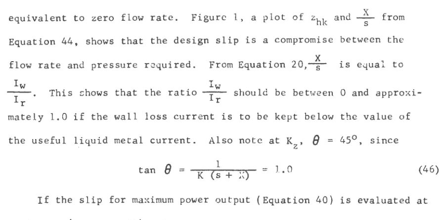
equivalent to zero flow rate. Figure 1, a plot of zhk and X s from
Equation 44, shows that the design slip is a compromise between the
flow rate and pressure r~quired. From Equation 20,--s-X is equal to
Iw
I .
r
Iw
This :::hows that the ratio ~ should be between 0 and
appro:xi-mately 1.0 if the wall loss current is to be kept below the value of
the useful liquid metal current. Also note at K ,
8
= 45°, sincez
tan
8
-=K-(r-s-+-:---:;..,...~)-1=
1 • 0 (46)If the slip for maximum power output (Equation 40) is evaluated at
optimum K (Equation 43) and at some preselected X, it is found that this
operating point is also one of maximum ideal electrical efficiency, i.e.
s
=
s0=
(x2+
X)~
- X ; se combining Equations 39 and 43 yieldsK
=
K ze=
1(39)
(47)
The equation of z0 can now be simplified by substituting for s and K from
Equations 39 and 47 respectively, to
This shows that the optimum value of the output utilization factor z0 is
equal to o~e half of the ideal electrical efficiency and that both z05
and Zok occur at the same slip. In the case of the head utilization
factor, it can be shown that zhs (occurring at sh) and zhk (occurring
at K2 ) cannot occur together; thus there is not a single optimum value
[image:32.601.95.543.111.334.2]Iii
a: 0.3
f2
~
Z
_I
_:...1~hk-2 I
+X-s
K - K • _...;.I __
-
z
s +X
O
0 0.1 02 0.3 0.4 0.5 0.6 0.7 OS
WALL LOSS PARAMETER
DIVIDED BY SLIP,
A:
b.
s
Ir
0.9 1.0
Figure 1. The variation of the maximum head utilization factor, zhk'
[image:33.599.123.500.50.702.2]B. Windings
The proper winding design will provide the field strength required
to meet the flow rate and slip used in the stator design calculations.
A particular winding configuration is checked by calculating the total
theoretical input impedance and the stator phase current at an assumed
input .voltage and slip. If the resulting ampere turns are sufficient,
this particular winding design would be acceptable. In order to find the
theoretical input impedance and stator phase current, the equivalent
circuit of the pump must be determined. Cage and Collins (11) assumed
that the equivalent circuit of an induction motor could be modified to
compensate for the case of a liquid metal rotor in a_pump duct. They
made the following modifications: the rotor leakage reactance was assumed
to be negligibly small; the power loss in the fluid channel walls was
added in parallel with the magnetizing reactance and the primary iron
loss was neglected since saturation in the iron is lo.w. An outline of
their results is shown below.
The primary resistance, Rl, per phase is
Rl Pcu Nl (MLC)
Primary leakage
=
Ac cp
reactance, xl, is obtained
2f qwB N 2 1
xl
=
---1-o-=7=----where the coil end leakage is
L s1 k 2
¢
c = _2_7T'_n_2
;;;.__w....t:~-from(49)
(50)
and the stator slot leakage is
The magnetizing reactance,
Xm•
is=
6. 06 x 1o-s
_f_<_N.=.l_k ... P;__kd=-)-2_A...;B;__ n2 g(52)
(53)
The equivalent resistance of pump duct walls referred to the primary on
a per phase basis is
w Rc
=
3p
w--:::"2-t;...w_-=L-When referred to the primary, the equivalent fluid resistance, R2 , is
(w
+
0.075 w)tL
+
Pcu0.64
nZ
(54)
(55)
Figure 2 shows the typical single phase equivalent circuit of a polyphase
flat linear induction pump with all rotor quantities referred to the
stator.
When designing windings for a flat linear induction pump, the
grad-ing of the magnetic field must be considered. It has been shown by
Blake (12) that end effects (i.e. abrupt changes in the magnetic field
at the ends of a linear pump with nongraded windings) cause the flux to
have a pulsating component. This component in turn adds a pulsating
component of current in the liquid; the current does not increase the output power but does increase the power loss in the liquid metal by the factor
(1 +
~)
over that of a pump with an ideally graded field. [image:35.601.91.532.40.430.2]Eg
IL
jXm
Rc
I
Figure 2. Single phase equivalent circuit of polyphase flat linear induction pump
R2
-
s
N [image:36.595.72.703.178.361.2]added heat loss to the liquid metal is too large even at relatively
large slips. For example,at a slip of 0.8 the power loss in the liquid
metal is nearly tripled.
These abrupt changes in the magnetic field at the ends of the pump
are overcome by many different methods of grading the winding. This
gradually increases the flux from zero at the ends to the uniform value
in the middle region. The windings may be graded over the entire length
of the pump, but this necessitates the separate design of each coil.
\•lindings may also be graded over just the end regions of the pump, thus
allowing the flux in the fully wound region to be of the ideal form.
A good example of the latter method is the double layer winding with
IV. THEORETICAL DESIGN OF PUMP
Based on the design theory of flat linear induction pumps and the
immediate performance requirements, it was decided that the pump under
design should be a five pole, one slot per pole per phase, full pitch,
twelve coil, wye connected, three phase pump with a double layer winding
on just one stator. This winding configuration automatically offers two
half wound end poles and three fully wound central poles.
Initially the designer of a linear induction pump is usually given
or must select certain operating conditions such as the working fluid,
temperature, duct material, flow rate, hydraulic losses in pump duct
acceptable, and approximate output pressure required-for the intended
application. The restrictions of hydraulic losses and pump duct
cavita-tion almost fix the overall reduction in area from the pipe to the pump
duct. And since the pipe area is known, so is the duct area. The ratio
of internal duct width and thickness is also restricted; virtually
es-tablishing these dimensions and the magnetic gap. From the duct area
dnd flow rate the fluid velocity in the pump region is determined. Now
the hydraulic losses can be checked. If these losses are satisfactory,
these dimensions may be used. It would be desirable to make the duct
thickness and the magnetic gap very small for maximum field
considera-tions; however, the resulting large hydraulic losses could not be
tolerated. Conversely, making the duct square and the resulting gap
large to reduce hydraulic losses would decrease the magnetic field in
The dimensions above and equations from design theory may now be
used to design an optimum stator structure. The optimum structure offers
maximum pressure development, maximum power, or maximum efficiency at the
given operating conditions. In this work the requirement of maximum
pressure development at a good efficiency was selected on the basis of
the intended installation of the pump in an operational sodium loop. The
factor zhs was not used since only the pressure output would be maximized.
Good efficiency would be obtained only by having a good power output.
Therefore, two methods of optimization~
0
=
z0s=
Zok• zh=
zhk andz0
=
z0k, zh=
zhk)were checked. Both methods simultaneously offereda maximum zh for high pressure output and a maximum z0 for good power
output after assuming or calculating the operating slip. The calculated
slip by the first method was found to be unsatisfactory for these pump
conditions. The second method (where z0 = z0k,zh = zhk• and K = Kz)was
the one actually used to design the flat linear induction pump.
The design of the pump was accomplished in two steps. First, as
discussed in the two preceding paragraphs, the optimum stator structure
for sodium at 400 C was established from calculations for maximum
utiliza-tion factors. Second, the parameters for the flat linear induction pump
equivalent circuit were determined for several winding configurations.
Based on these equivalent circuits, the winding method was determined
that most nearly offered the ampere turns assumed in the first step.
A. Optimum Stator Structure
The induction pump was designed for operation with sodium metal at
area from 0.75-inch schedule 40 inconel pipe to the duct was made slightly
less than three to one in accordance with Watt (13). Larger reductions
could cause cavitation (i.e. a condition existing when inlet pressure
falls below the vapor pressure of the fluid and resulting small cavities
of vapor collapse in the pump duct). The design performance criterion
was approximately five gallons per minute flow rate of molten sodium.
The various dimensions and material properties used were
f = 60 cps
g = 0. 794 ern
k
=
1/302 stokes~ = 1
t
=
0.318 erntw
=
0.158 ernw = 3.81 ern
~
=
0.00284 poise (14)p
= 21.93 microhm ern (14)Pw
= 98.1 microhm ern (15)u
=
0.857 grams per cc (14)In order to obtain a strong field, a small air gap, g, was selected;thus
the internal thickness, t, of the pump duct was also small. The internal
width, w, was chosen so that the ratio of _!_ would be greater than 10.
The resultant f111id velocity was approximately 260 em per second at the
design flow rate using the equation
v=~
wt
At this velocity the Reynolds number was 46,250 using the equation
vd
R e
=
~(56)
(57)
and the resulting theoretical hydraulic loss was satisfactory at 0.46 psi
per foot of pump duct.
Initially an attempt was made to optimize the output utilization
factor, z0 , for maximum output at the slip of maximum efficiency and tO
maximize the head utilization factor, zh, at Kze· Using Equation 21
the wall loss parameter, X, is 0.223. The slip, found from Equation 39
with X
=
0.223, is s=
se=
0.300. The pump parameter K=
Kze=
1.91is determined from Equation 47 with X
=
0.223. From Figure l withX
-s;-
=
0.744 observe that zhk=
0.287 which is a relatively low maximumzh. Finally the wavelength, A , is found to be 29.6 em via Equation 18.
The velocity of the magnetic field is computed from the Equation vs
=
fA;thus vs = 1778 em per second. At se, v
=
1241 em per second whichgreatly exceeds the assumed fluid velocity of 260 em per second. In
addition this high fluid velocity, equivalent to 23.4 gpm, probably
could never be attained experimentally due to the severe hydraulic losses.
Now assume that this pump was built, but let the operation be such that
v
=
260 em per second or s = 0.855. Thus K = Kze = 1.91, sI
se,and 42,zh
=
0.311 and z0=
0.045. This may appear to be a satisfactorydesign. However, before selecting a design consider a pump operated at
the design value of slip.
At this point it was apparent that for the design to be practical
the slip must be increased, but the extent of this increase was not
known. In this case both utilization factors were maximized at optimum
K since this method allowed different slips to be tried. It was then
necessary to find a slip which satisfied the conditions of optimum K
and a liquid velocity of 260 em per second. First note that
v
vs
=
-r:s-
= f ). (58)and therefore
). = --::-f
-:(~~
--s-:-)- (59)The optimum K is obtained from Equation 43. Combining Equation 18,
the pump parameter, with the Equations 43 and 59 yields the following
1
_ _..;;; __ =
ftX+ s 2Tr
gp
52 - 2
8
+
1 s+
8
- X = 0(60)
8
8
where
8=
2Tr ge.
fJl-o
v2 tEquation 60, a quadratic, is easily solved for the slip s
= 0.81.
Sincev
=
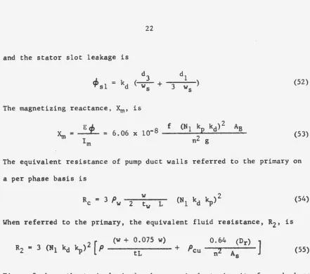
260 em per second was approximate, a design slip of 0.80 was assumedshows the value of zhk• in this case 0.392, to be very near the maximum
value since X is never zero. The corresponding value of z0k was 0.078.
The optimum K (Equation 43) is now found to be 0.976. This value of
K is shown to produce a maximum zh in Figure 3 by plotting values of zh
from Equation 41 at various values of K. When this value is
substi-tuted into Equation 18, the result is ~= 21.2 em. It is obvious
now that the design and operation o~ the pump at the same slip is
beneficial. The second design method yielded a higher zh and increased
Z0 by almost a factor of two. The wavelength was shorter by the latter
method which allowed the five pole pump to be 54.8 em long rather than
75.8 em long; this was a very significant result. Thus the overall
length of the five pole pump was 54.8 em with equal slot and tooth
dimensions of 1.766 em. The nominal stator width was determined by
the combined thickness of 91 laminations of 24 gauge hot rolled high
silicon magnet core iron insulated from each other with 0.004-inch mica
sheet.
The stator structure design for the linear induction pump was still
not completely determined since the slot depth was unknown. However,
all necessary dimensions were available for the design of the pump duct.
This is shown in Figure 4.
B.
WindingsThe next logical step in the design of the flat linear induction
pump was the determination of the exact winding configuration (i.e. the
required number of turns per coil and the electrical connections). It
~
~0.3
z
0
ti
~0.2
§
Q
c
Ql
L&J
:J:
.5
It<
z
h •
I
+
t1t< 1
(I
+t
)I
• • 0.8
X • 0.223
1.0
1.5
2.0
3.0
PUMP PARAMETER, K
Figure 3. The variation of the head utilization factor with the pump parameter
w
[image:44.597.170.532.158.443.2]~-"""'"•
~
! [
---
... .. ---
=
. .
~
i
- --- - s"~ ---~··---
-r
- - ~·- _j~
-f -----
~
7d
?
I I ' -~
1
L
.~
-- ---·"
4 0 •N0-000"-'·
_z.,
I I
I
l _ j _I I I I ·""'
' '
---.-1""-'C.ONS\....
.,.._· ,. '/•~ ~~~';.s;.~ .~6~ c~~~~~T''·""rv ..
~- A-.A
PUMP :a&.C..T\ON
NO"T&~; I. '-e'"""Or-T""" 0~ PIOE !l>ec,TIOW~ ...,,'-'- V.etr.£.V Pat.lO•N.-, Tl.lS.
1"-la.-.T•OM .,.. pUMP bVC."T \....n-0 L-OOP·
2 . ~0\....C•a COPPa.lt. Bu . . . ._~ T~ OuMP ~ec..,-oc.
MI.__ ..,_&1.-'T•~• 'l=OQI ... T · ••'-\.l&lk ::::.0'-0.111..,.
Figure 4. Pump duct for flat linear induction pump
w
[image:45.593.44.718.38.521.2](0.0808-inch diameter) heavy formvar insulated copper magnet wire. Since the liquid flow can be throttled to the design rate and the ultimate test
loop can withstand pressures up to 100 psi, a design gross pressure of
60 psi at 0.8 slip and 250 volts line voltage was used. Based on the
performance of other pumps the actual pressure developed by the pump was
expected to be from 40 to 80 percent of this design figure.
The required number of ampere turns per phase was determinE!d from the equation formed by the substitution of Equation 12 for Is into
Equation 28. This result, after Equation 28 is multiplied by x to
convert p to gross pressure, is
( 4 p t g n2 ~
288
J.L
o
x ?.h~
) (61)
The solution of Equation 61 with p
=
60 psi, t=
0.318 em, g=
0.794 em,n = 5 poles, ~ = 21.2 em, - 4-J-Lo 1.451 x lo-7, x
=
31.8 em (fullywound region), and zh = zhk = 0.392 yields NpH I= 3,920 ampere turns
per phase.
The various constants, dimensions, and physical properties used in
the following winding design calculations are
Ac 0.0049 in. 2
As 0.0625 in. 2
f 60 cps
g 0.311 in.
kd 1.0
kp 1.0
(MLC) 12.5 in.
q 3
sl 15
ss 15
t 0.125 in.
tw 0.0625 in.
w 1.5 in.
WB = (2. 660) (0.9) in. ws = 0.695 in.
p
= 8.64 microhm in. (14)Pcu
= 1.65 microhm in. at 400 C (15)Pcu
=
0.827 microhm in. at 75c
(16)Pw
=
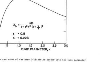
38.6 microhm in. (15)The first winding configuration tried was one consisting of 120 turns
per coil with one coil in series per phase and four circuits in parallel
per phase. Using Equation 49 with cp
=
4 circuits in parallel andN1
=
240 series conductors per phase, the primary resistance, R1 , is0.127 ohms. The primary leakage reactance,
x
1 , is found to be 1.08 ohmsfrom Equations 50, 51, and 52 where d1 = 2.16 in. and d3
=
0.34 in. It is necessary to change the slot depth, d1+
d3 , for different windingdesigns since a space free of conductors is required for forced air
cooling of the pump. When the area of the gap, AB
=
LwB=
51.6 in., issubstituted into Equation 53, the magnetizing reactance,
Xm•
isequivalent fluid resistance, R2 , are 3.72 ohms from Equation 54 and
2.14 ohms from Equation 55 respectively.
It should be mentioned here that the assumption of negligible rotor
reactance has been shown by Blake (12) to be good if the ratio of ~
is less than 0.1. The ratio ~ for this particular induction pump
is 0.015.
The magnitude of the total pump impedance per phase,
I ztl
=
2.14 ohms,is determined from the equivalent circuit, Figure 2, using alternating
current circuit analysis at the design slip of 0.8. Dividing the phase
voltage, E~= 144 volts, by
IZrl
yields the total phase current,I,
of 67.4 amperes. Thus the resultant ampere turns per pbase for thiswind-ing configuration are 8, 080 which are more than is required. The current
per coil must also be checked since the maximum allowable current for
12 gauge wire is 20 amperes. In this example the current per coil is
16.8 amperes.
Several other winding configurations were investigated before one
was found with an ampere-turn rating approaching the design value of
3,920. The results of these investigations are summarized in Table 1.
Based on the data shown in Table 1, the 60 turns per coil winding
method was obviously the only one meeting all of the specifications.
Even though this method provided slightly more than 3,920 ampere turns
per coil, it was adjudged unnecessary to further reduce the turns per
No. of
turns/coil
120
80
60
No. of
turns/coil
120
80
60
No. of series turns/phase
120
160
240
s
I
z-r
I
ohms
0.8 2.14
0.8 4.04
0.8 8. 72
cp Rl ohms
4 0.127
2 0.338
1 1.01
Ec/>
Ivolts amperes
144 67.4
144 35.6
144 16.5
xl ohms 1.08 2.08 4.11 xm ohms 2.17 3.86 8.68
Coil current amperes
16.8
17.8
16.5
Rc Rz
ohms ohms
3. 72 2.14
6.60 3.81
14.87 8.56
[image:49.595.76.640.129.546.2]a-Figure 5 shows the complete flat linear induction pump design. Note that the stator without windings, sometimes called the "core", is almost
the same size as the stator with windings; however, it has no slots.
The electrical winding connections are shown pictorially in Figure 6.
C. Theoretical Performance Characteristics
The theoretical performance characteristics of the induction pump
were computed using the equivalent circuit parameters for a winding
with 60 turns per coil. The stator phase current was determined as
before except the slip was determined from the equation
Q
s
=
1 - --=-2 4.,..._---=3~5- (62)as the flow rate changed. In this case the phase voltage was also
varied. Thus to each value of flow rate and line voltage there was a
corresponding unique value of stator phase current.
If the stator phase current, I, is substituted into Equation 12,
the value of the stator surface current per unit length, Is, is obtained.
The dimensions and material constants are as listed on page 26. The pump parameter, K, is 0.976. The stator surface current, Is, is then used in
the evaluation of the gross pressure developed over the fully wound region
of the pump stator via Equation 28 multiplied by x = 31.8 em (i.e. the length of the fully wound region). When the hydraulic losses, Pf' in the
pump duct are deducted from the gross pressure, xp, the resulting value
is the actual theoretical pressure developed, (p) ac ua t 1 , by the induction
pump. Equations 31 and 32 provide the actual power output in the
~
~
~
,.
+
+
t
'
1I
:-:::
.. , ..
,!"~::~
I
I
ll
· - - · - - - -Zt.!IW 'l"
• 4"LG, ~'!'UCTUD'b~CT\.OWNCO.) -,'i, ~11.-L. T~~U TOOT~
(Toe&e.&"IVE •""-!lit .... c
I C. ~.,jOt,..$
~
'
/ /,... .
/ ·~
----1---_/
~ ~ 1
l"a,F
I
~I!TI.. .. ..,.IN.\·
T,Cf><O~~
L _ _ _ __ _ _ _ _ _ __ _ _ _ _ _ - - - 1 - - - '
=
UO -~-UTOONc~··-•T) :::t:; .
1=•8Eit""6.~R T~ p,,-1!1,,_ e.~L T CRO~·--c• 0<-1
~'
n / o.ooi T<. ""<•rJ
~ ~ ~
1
~~~
-~
~[~v
~;~~~~~:~=~--T
-I~~
,! \ coae••~
U
i'li:
I, l • ...-E\IER't' "H ... La.lroii ... TIO,_.l! ~;~=~e:c!;:v.,,, ..
ONIE. L 6.lAII\llli.TION 00.0. ~ ....OT Ell TENC)
..
~ oen .. L T~o~tt.u aooT
(TOR-e:HW•IO-~£ .. ~ • • ·~,..-.. 3TUO'T\.IC"D 80TI.t liit.:tO~·)
.~ .... ~~~
Figure 5. Stator and core design for flat linear induction pump
~·
~
.-\._ -,.~ ,_O,t.11"-llo.T•LN 'T""o":
~ CE NOT E'•TElo.~_ec
(T '0' P eoT .... PI&'-.... :
w
[image:51.599.72.694.80.483.2]c
c
a
b~
c
'A.,
2
b
b a
....
----'A.----~c
bn n n
a
c
b
a
c
bc' c" c'"
Figure 6. Winding connections for flat linear induction pump
[image:52.601.68.537.49.705.2]