Truck to door sequencing in multi door cross docking system with dock repeat truck holding pattern

(1)

* Corresponding author Tel. : +61488122440 E-mail: [email protected] (A. Ardakani) 2020 Growing Science Ltd.

doi: 10.5267/j.ijiec.2019.10.001

International Journal of Industrial Engineering Computations 11 (2020) 201–220

Contents lists available at GrowingScience

International Journal of Industrial Engineering Computations

homepage: www.GrowingScience.com/ijiec

Truck-to-door sequencing in multi-door cross-docking system with dock repeat truck holding pattern

Allahyar Ardakania*_{, Jiangang Fei}a _{and Pedram Beldar}b

a_{National Center for Ports and Shipping, Australian Maritime College, University of Tasmania, Tasmania, Australia} b_{Department of Industrial and Mechanical Engineering, Qazvin Branch, Islamic Azad University, Qazvin, Iran} C H R O N I C L E A B S T R A C T

Article history: Received May 22 2019 Received in Revised Format August 29 2019

Accepted October 12 2019 Available online October 12 2019

Cross-docking is a logistics strategy that consolidates the products of different inbound trucks according to their destinations in order to reduce the inventory, order picking, and transportation costs. It requires a high level of collaboration between inbound trucks, internal operations, and outbound trucks. This article addresses the truck-to-door sequencing problem. Truck-to-door sequencing has been studied by some researchers in different titles such as scheduling and sequencing of inbound and outbound trucks of the cross-dock center. However, previous studies have not considered repeat truck holding pattern. Therefore, it is important to determine the doors and the sequence of the inbound and outbound trucks that should be assigned in a cross-dock center. This paper focuses on optimizing truck-to-door sequencing with consideration of repeat truck holding pattern in inbound trucks in order to minimize makespan. Two methods are considered to solve this problem, including mathematical modeling and a heuristic algorithm. In the first method, a mixed integer-programming model is developed to minimize the makespan. Then, GAMS software is used to solve small-scale problems. In the second approach, a heuristic algorithm is developed to find near-optimal solutions within the shortest time possible and the algorithm is used to solve large-scale problems. The results of the mathematical model and the heuristic algorithm are slightly different and show the good quality of the presented heuristic algorithm.

Keywords: Cross-docking

Dock Repeat Truck Holding Pattern

Heuristic Algorithm Truck-to-door Sequencing Multi-door

Makespan

1. Introduction

(2)

Cross-docking is divided into three-decision levels, which are strategic (Long term), tactical (mid-term), and operational levels (short term). Different research questions have been raised in these decision levels, but the operational level is the most attractive part for scholars and has been developed into the five research areas (Boysen & Fliedner, 2010; Van Belle et al., 2012). Dock-door assignment or Truck-to-door assignment tries to allocate trucks to doors optimally, and the time is considered not important.

Truck scheduling includes the time dimension but does not take into account the order of trucks. Truck sequencing only considers the sequence of trucks. Truck-to-door scheduling only takes into account at which door and at what time the truck should be docked. Truck-to-door sequencing tries to address which door and in which order the truck should be docked when an inbound truck arrives at the cross-dock center (Ladier & Alpan, 2016; Van Belle et al., 2012).

When the problem of truck-to-door sequencing is mentioned, two different questions should be answered: at which door and in which order the trucks should be docked. Several scholars only answered the first question which has been called as truck-to-door assignment (Nassief et al., 2016; Yu & Egbelu, 2008), while others answered the second question, which has been considered as truck sequencing (Dondo & Cerdá, 2013; Fazel Zarandi et al., 2016; Larbi et al., 2009; Yazdani et al., 2015). Most studies tried to solve the cross-docking problems with one inbound and outbound door (Boloori Arabani et al., 2011; Cóccola et al., 2015; Liao et al., 2012; Maknoon & Baptiste, 2009; Yu & Egbelu, 2008), which is impractical in the real world (Wisittipanich & Hengmeechai, 2017). In general, the literature on truck-to-door sequencing focuses on the order or sequence of trucks and the doors which trucks should be assigned, In order to simulate real cross-dock operations, scholars should consider planning and scheduling problems with a realistic number of trucks and doors (Dondo & Cerdá, 2014; Shahin Moghadam et al., 2014; Wisittipanich & Hengmeechai, 2017). Li et al. (2004) presented research as a two-phase parallel machine scheduling problem with earliness and tardiness in an integer programming model. In this model, the jobs were trucks and doors were machines. This research aimed to process the trucks close to their due date and minimize the total deviation. McWilliams and his co-authors presented several studies related to truck-to-door sequencing (McWilliams, 2005, 2009, 2010; D. L. McWilliams, 2009; McWilliams. et al., 2005, 2008) in Paracel industry that included the scheduling of inbound trucks which after unloading, the products were transferred to the outbound trucks with conveyors. The research aimed to minimize the period with different assumptions. As a method, the author used a Genetic Algorithm (GA) in the simulation. In another study, McWilliams (2005) used a Simulated Annealing (SA) to solve the same problem. In continue of their research, they relaxed the assumption of the same size parcel and unloading time for all the inbound trucks, but the objective was the same (McWilliams et al., 2008).

(3)

cargo shipment, and total capacity at the cross-dock center. This paper aimed to find the optimal sequence of trucks in order to minimize the operational cost of shipments and unfulfilled shipments.

Konur and Golias (2013) presented a bi-level optimization problem for pessimistic and optimistic approaches. The arrival time of inbound trucks are unknown, and in order to sequence the inbound trucks Genetic algorithm was proposed. Kuo (2013) developed a model intending to solve the sequencing and assignment of the inbound and outbound trucks simultaneously. In order to minimize the makespan, a variable neighborhood search algorithm was used. Madani-Isfahani et al. (2014) conducted a study with multiple cross-dock, assuming that each truck could be assigned only to one door, and there was one temporary storage with unlimited capacity. The aim was to minimize the makespan. The metaheuristic algorithm, such as simulated annealing and firefly algorithms was used to solve the problem. In continue, Wisittipanich and Hengmeechai (2017) proposed a truck scheduling problem in the multi-door cross-docking terminal. They presented a Mixed Integer Programming (MIP) model for minimizing the makespan and then solved the model with a modified PSO Meta-heuristic algorithm. In continue, Molavi et al. (2018) presented a truck scheduling model in a cross-docking area with consideration of fixed due dates. The proposed model was a MIP model, and in order to solve, they considered a hybrid genetic algorithm-reduced variable neighborhood search. The objective of the research was minimizing the delayed shipments and delivery cost of retained products.

To the best of our knowledge with reviewing the literature and according to the literature provided by Ladier and Alpan (2016), Wisittipanich and Hengmeechai (2017), and Ye et al. (2018) on truck-to-door sequencing, this paper is the first study that focuses on truck-to-door sequencing problem with consideration of pre-emption and continues the research presented by Wisittipanich and Hengmeechai (2017). A truck holding pattern can help managers have freedom in changing the sequence of trucks when they are faced with an uncertain environment. The paper is organized as follows. The problem is described in details in the next section, after which a section related to assumptions has been presented. A Mixed integer model is proposed and solved with GAMS software. Also, because the problem is NP-hard in a strong sense, a heuristic algorithm is developed. Finally, numerical result, conclusion, and future research are presented.

2. Problem Description

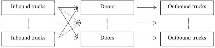
[image:3.612.95.447.608.687.2]

This study has been carried out to make a model according to the problem suggested by Yu (2002). Makespan refers to the time when the first product is unloaded from an inbound truck to the time when the last product is loaded in an outbound truck in cross-dock center. It must also be noted that secondary activities, such as labeling, and preparation, are not considered in this model. When inbound trucks enter the cross-dock center, all their products are unloaded. Then, products are transferred to outbound doors by the transfer system (conveyers or workers) and loaded in the outbound trucks. Here, there are several doors in the cross-dock center (Fig. 1). The inbound trucks enter the cross-dock center are assigned to inbound doors. Inbound trucks can move between doors, but the outbound doors are fixed. When assigned to outbound doors, each outbound truck stays in the same door until its capacity becomes full. Then, products are shipped to their respective destination. There is no space in the model for temporary storage.

Fig. 1. Assignment of inbound and outbound trucks to doors Inbound trucks

Inbound trucks

Doors

Outbound trucks

(4)

2.1. Assumptions

The following assumptions are considered in this model:

1. Inbound and outbound trucks are presented in a cross-dock at a certain time t=0. They can be assigned to various doors simultaneously.

2. All inbound products must be transferred to outbound trucks without storage. This transfer is usually applied to fresh or frozen food products requiring temperature control.

3. The number of receiving products equals the number of shipping products. 4. There is no priority for products regarding loading and unloading.

5. It is also possible to unload receiving products as much as outbound trucks capacity. In other words, inbound truck 1 has 100 units of product 2 and 30 of product 3. The outbound truck only needs 80 units of product 1. Only the same 80 units are transferred, and the inbound truck leaves the doors and waits for the next assignment.

6. Inbound trucks stay at entrances only when the outbound trucks’ needs are satisfied. Outbound trucks have no time limit for staying at exits.

7. No time is considered for secondary operations like product identification and labeling. Hence, it is assumed that immediately after the entrance of inbound truck, it can transfer its load to the dock and outbound truck.

8. Loading and unloading time of all products are the same for inbound and outbound trucks. 9. Delay time for changing all inbound and outbound trucks is the same and constant.

10.Constant time is considered for transferring products from an inbound truck to the outbound equal to one unit of time.

11.If trucks are displaced between two doors, docks change considered rather than truck change. Its value is different from the trucks changes.

3. Mathematical Modelling

The above assumptions were used for modeling the problem. Also, it was assumed that the number of inbound and outbound trucks must be more than the number of doors to simulate a real-world problem.

3.1. Parameters

n Number of products

m Number of doors

q Number of inbound trucks

u Number of outbound trucks

k Index for products where k



1, 2, , n



,

l l Index for doors where l l, 



1, 2, , m



,

i h Index for inbound trucks where i



1,2, , q



,

j e Index for outbound trucks where j



1, 2, , u



, i k

r Number of units of product k loaded in the inbound truck i

, j k

s Number of units of product k needed for outbound truck j

, l l

t  Transportation time from door l to door l.

d Truck changeover time

v Transportation time of products from inbound doors to outbound doors

3.2. Binary Variables

, , i j l

Y Binary variable taking value 1 if any product transferred from inbound truck i to outbound truck j

(5)

, , i h l

Z Binary variable taking value 1 if inbound truck i precedes inbound truck h at the door l, and 0 otherwise. i q h i,

, j e

W Binary variable taking value 1 if outbound truck j precedes outbound truck e; and 0 otherwise. ,

j u e j

, i l

H Binary variable taking value 1 if inbound truck i visits door l; and 0 otherwise.

, j l

L Binary variable taking value 1 if the outbound truck j is assigned to the door l, and 0 otherwise.

, , i l l

G  Binary variable taking value 1 if inbound truck i visit door l before the door l; and 0 otherwise. ,

l m l l .

3.3. Continuous Variables

1 ,

i l

E Continuous variable for starting time of unloading the inbound truck i at the door l.

2 ,

i l

E Continuous variable for finishing time of unloading the inbound truck i at the door l.

1

j

F Continuous variable for starting time of loading outbound truck j.

2

j

F Continuous variable for finishing time of loading outbound truck j. max

C Continuous variable for makespan

3.4. Integer Variables

, , , i j k l

X Integer variable for the number of units of product k transferred from inbound truck

i to outbound truck j at the door l. Xi j k l, , , .

3.5. Mixed Integer Programming Model

In this section, the mathematical model is presented:

minCmax (1)

subject to:

, , , , 1 1

u m

i j k l i k j l

X r

 





i k, (2)

, , , ,

1 1

q m

i j k l j k i l

X s

 





j k, (3)

, , , , ,

1

*

n

i j k l i j l

k

X M Y







i j l, , (4)

, , ,

1

*

u

i j l i l

j

Y M H

 



i l, (5)

, 1 1 m j l l L  



j (6)

, , ,

1

*

q

i j l j l

i

Y M L

 



j l, (7)

2 1

, , , , ,

1 1

u n

i l i l i j k l

j k

E E X

 

(6)





1 2

, , , 3 , , , ,

i l i l l l i l l i l i l

E E t M G H H  i l m l l, , (9)





1 2

, , , 2 , , , ,

i l i l l l i l l i l i l

E  E t M G H H  i l m l l, , (10)





1 2

, , 3 , , , ,

i l h l i h l i l h l

E E  d M Z H H i q h i l, , (11)





1 2

, , 2 , , , ,

h l i l i h l i l h l

E E  d M Z H H i q h i l, , (12)

2 1

, , ,

1 1 1

q n m

j j i j k l

i k l

F F X

  

 



j (13)





1 2

, , ,

3

j e j e j l e l

F F  d M W L L j u e j l, , (14)





1 2

, , ,

2

e j j e j l e l

F F  d M W L L j u e j l, , (15)





2 1

, , , , , ,

1

n

j i l i j k l i j l

k

F E v X M Y



  



  i j l, , (16)

2

max j

C F j (17)

The objective, as presented by Eq. (1), is to minimize makespan. Constraint (2) states that the total number of product k transferred from inbound truck i to all outbound trucks at door l is the same as the number of product k first loaded in inbound truck i. Similarly, constraint (3) states that total number of product k transferred from all inbound trucks to each outbound truck j at door l is the same as the number of product k required for each outbound truck j. Constraint (4) establishes proper relationship between transfer variable Yi,j,l and decision variable Xi,j,k,l. Constraint (5) states that a product will be transferred

from the truck i to truck j at door l if inbound truck i is assigned to door l. Constraint (6) states that each outbound truck j is only assigned to a door and stays in the same station until it is fully loaded. Constraint (7) states that if outbound truck j is assigned to door l, it will be possible to load product to the outbound truck. Constraints (8), (9), and (10) control the assignment and entering and leaving time of inbound trucks. It should also be mentioned that constraints (9) and (10) indicate the repeat truck holding pattern in inbound trucks. Constraint (11) and (12) control the sequence and entering and leaving time for inbound trucks. Constraints (13) to (15) control the sequence and leaving time for the outbound trucks. Constraint (16) shows the relationship between the leaving time of outbound trucks and entering time of inbound trucks if a product is transferred. Constraint (17) considers the completion time as the same as the time of the last outbound trucks leaving outbound doors.

4. Solution method

Heuristic Algorithm

(7)

trucks and updating the table is carried out to the satisfaction of inbound and outbound trucks. Heuristic algorithms with six SC are as follow:

1. SC1: maximum products transfer

2. SC2: maximum ratio between products transfer 3. SC3: maximum fit between products transfer

4. SC4: maximum products transfer regarding priority condition 5. SC5: maximum products transfer ratio regarding priority condition 6. SC6: maximum fit between products transfer regarding priority condition

SC 1, 2, and 3 comply with the same trend except for the time when the algorithm seeks for selecting the same number of trucks as doors. In each reiteration, the most suitable trucks are selected based on selection criteria. SC 4, 5, and 6 are partially changed versions of SC 1, 2, and 3. They follow the same rules as SC 1, 2, and 3 but have a priority condition regarding the assignment. In reiterations of this algorithm, if there is a set of trucks meeting priority condition, SC 1, 2, and 3 will be computed for the trucks. Then, the best trucks are selected among them. Otherwise, in reiterations, the algorithm will automatically change into algorithms 1, 2, and 3. It should be noted that our study considers a different problem based on the presented method by Yu (2002). The main difference is in the selection of each pair as we have more than one door, so we need to select trucks according to the number of doors. The method for updating the trucks as we have repeat truck holding pattern. Finally, in order for calculating the makespan because it is completely related to a penalty that will pay for changing trucks.

Priority conditions

In priority condition, assume that a certain type of product is only placed along with the sequences of an algorithm in an inbound truck. This indicates that all outbound trucks requiring that product are paired with the inbound truck carrying that product. For instance, assume that we have four inbound trucks, four outbound trucks, and two doors. In algorithm reiterations, product 3 is only loaded on inbound truck 4. Trucks 1, 2, and 3 do not carry product 3. Outbound trucks 2 and 3 need product 3. Outbound truck 1 and 4 do not need product 3. Hence, outbound trucks 2 and 3 must be paired with inbound truck 4. The same rules must also be considered for outbound trucks. Assume that an outbound truck receives only one type of product. Other outbound trucks do not need that product, however. All inbound trucks with that particular product are paired with that outbound truck needing that product.

4.1. SC 1 -maximum products transfer

For the heuristic algorithm, we calculate the total number of products which can be transferred from inbound trucks to outbound trucks for all pairs. Then, we select the pair with a maximum number of products transferred from inbound trucks to outbound trucks. It must be noted that the number of inbound trucks is selected based on the number of existing doors. For instance, if we have three doors, three trucks must also be selected in each reiteration unless there is no inbound or outbound truck to be selected. Upon the selection of the best set of trucks, the number of products remained in inbound trucks and the number of products required for outbound trucks is updated for the following reiterations. These reiterations will continue until the satisfaction of inbound and outbound trucks.

Heuristic Algorithm with SC 1

(8)



, ,



1

,

N

ij i k j k

K

min r s

 





(18)

ij

 : Total product units transferred from an inbound truck i and outbound truck j

, i k

r : Total units of product k loaded in the inbound truck i in algorithm reiterations

, j k

s : Total units of product k required in outbound truck j in algorithm reiterations

Step 2: If all _ijequal 0, the algorithm is stopped. A response is obtained for the model. Otherwise, if there is any non-zero _ij, those pairs (as the same number as doors) with maximum _ij are selected. If some cases have the same amount, the most suitable pairs are selected after calculation.

Step 3: The number of products remained for inbound and outbound trucks is updated and then go back to Step 1.

4.2. Heuristic Algorithm with SC 2 -Maximum Ratio between Products Transfer

Here, the between-pair ratio _ijis expanded for selecting pairs. The ratio _ij for inbound trucks i and outbound truck j is defined as follow:

, ,

0 0

1

, ,

,

min

max ,

i k j k

r or s

N

i k j k

i k K

ij N

j k K

r s

  

 

 

 

 

 

 

 



 



(19)

ij

 : Ratio for inbound trucks i and outbound truck j pair

, i k

, j k

Given that if the denominator is 0, the total term will be considered 0.

Pairs ratio ij can be considered as the correlation between inbound trucks i and outbound truck j. ij

ratio interval is between 0 and 1. _ij=0 indicates that there is no relationship between inbound and outbound trucks. On the other hand, the outbound truck needs no product from the inbound truck. Yet,

ij

 =1 indicates that the number and type of products are the same for inbound and outbound trucks.

Step 1: For each pair of inbound trucks i and outbound truck j, inbound trucks i and outbound truck j

ratio is calculated by Eq. (19).

(9)

Step 3: The number of products remained for inbound and outbound trucks is updated and then go back to Step 1.

4.3. Heuristic Algorithm with SC 3 -Maximum Fit between Products Transfer

Pairs fit _ijwas established for SC 3. It can be considered as a correlation between inbound and outbound trucks. Yet, it differs from SC 2 in that _ijprovides the same weight from the type of products regardless of number of products loaded.

ij

 ratio interval is between 0 and 1. _ij=0 indicates that there is no relationship between inbound and outbound trucks. On the other hand, the outbound truck needs no product from the inbound truck. Yet,

ij

 =1 indicates that the number and type of products are the same for inbound and outbound trucks. _ij

fit for inbound and outbound pairs is stated as follow:

, ,

0 0

1

, , , ,

min max

1 , ,

i k j k

r N

K r o s

K r or s

N

i k

i

k

k j

j

i k j

r s

  

 

 

 

 

 

 

 





(20)

ij

 : Inbound truck i and outbound truck j pair fit

, i k

, j k

Denominator indicates a number of products loaded in the inbound truck i and outbound truck j.

Given that if the denominator is 0, the total term will be considered 0.

Step 1: For each pair of inbound truck i and outbound truck j, inbound truck i and outbound truck j fit is calculated by Eq. (20).

Step 2: If all _ij=0, the algorithm is stopped. A response is obtained for the model. Otherwise, if there is any non-zero_ij, those pairs (as the same number as doors) with maximum _ij are selected. If some cases have the same amount, we will calculate this problem and select the best result.

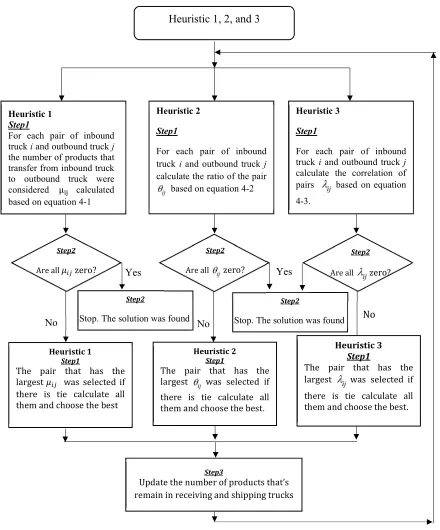
Step 3: We update the number of products remained for inbound and outbound trucks and went back to Step 1. As also mentioned in previous sections, heuristic algorithms 1, 2, and 3 follow the same trends. Yet, they apply different rules for selecting the best pairs. Fig. 2 illustrates a heuristic algorithm function in a stepwise manner in a flowchart.

(10)

Step 2: If a pair satisfying priority condition is identified, we go to 2-a. Otherwise, we go to 2-b.

2-a: We use a heuristic algorithm with SC 1 on pairs satisfying priority condition. Then, we go to section 1. Also, it should also be noted that if you have to select three pairs and three doors, yet you have two pairs based on priority condition, you obtain the third pair from 2-b.

2-b: We use a heuristic algorithm with SC 1.

[image:10.612.65.505.172.702.2]

Step 3: We update the number of products remained for inbound and outbound trucks. Then, we go to step 1.

Fig. 2. Flowchart of the heuristic algorithm with SC 1, 2, and 3 adopted from (Yu & Egbelu, 2008)

Heuristic 1, 2, and 3

Heuristic 1 Step1

For each pair of inbound truck i and outbound truck j

the number of products that transfer from inbound truck to outbound truck were considered μ calculated based on equation 4-1

Heuristic 2

Step1

calculate the ratio of the pair based on equation 4-2

Heuristic 3

Step1

calculate the correlation of pairs based on equation 4-3.

Step2

Are all 𝜇 zero?

Step2

Stop. The solution was found

Heuristic 1 Step1

The pair that has the largest 𝜇 was selected if there is tie calculate all them and choose the best

Step3

Update the number of products that’s remain in receiving and shipping trucks

Step2

Stop. The solution was found

Heuristic 2 Step1

The pair that has the largest was selected if there is tie calculate all them and choose the best. Yes

No

Yes

No No

Step2

Are all zero?

Step2

Are all zero?

Heuristic 3

Step1

(11)

4.5. Heuristic Algorithm with SC 5-Maximum Products Transfer Ratio in Priority Condition

It is precisely the same heuristic algorithm with SC 2; except pairs satisfying priority condition in algorithm reiterations. Priority conditions are considered for these pairs. They are executed in heuristic algorithm 2 for pairs. Otherwise, a heuristic algorithm with SC 5 changes into heuristic algorithm 2 in that reiteration.

Step 1: We identify all pairs meeting priority condition. That is, if only a certain product exists in only one truck, we identify all pairs requiring that product for loading and if a product is received by a truck, all trucks able to load to that truck.

2-a: We use a heuristic algorithm with SC 1 on pairs satisfying priority condition. Then, we go to section 1. Yet, it must also be noted that if, say, you have to select three pairs and three doors yet you have two pairs based on priority condition, you obtain the third pair from 2-b.

4.6. Heuristic Algorithm with SC 6-Maximum Products Transfer regarding Priority Condition

It is exactly the same heuristic algorithm with SC 3; except pairs satisfying priority condition in algorithm reiterations. Priority conditions are considered for these pairs. They are executed in a heuristic algorithm with SC 3 for pairs. Otherwise, a heuristic algorithm with SC 6 changes into heuristic algorithm 3 in that reiteration.

Step 1: We identify all pairs meeting priority condition. That is, if only a certain product exists in only one truck, we identify all pairs requiring that product for loading and if a product is received by a truck, all trucks able to shipload to that truck.

2-a: We use a heuristic algorithm with SC 1 on pairs satisfying priority condition. Then, we go to section 1. It must also be noted that if, say, we have to select three pairs and three doors yet we have two pairs based on priority condition and we obtain the third pair from 2-b.

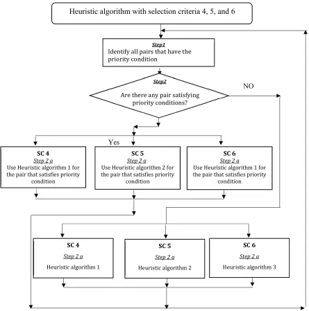
Fig. 3 illustrates a heuristic algorithm with selection criteria 4, 5, and 6 functions in a stepwise manner in a flowchart.

5. Makespan

(12)

[image:12.612.65.510.44.493.2]

Fig. 3. Flowchart of the heuristic algorithm with SC 4, 5, and 6 adopted from (Yu & Egbelu, 2008).

5.1. Notation

:

T Makespan

 2i l, :

E _{When inbound truck i in the inbound truck sequence leaves the receiving door.}

2_:

j

F _{When outbound truck j in the outbound truck sequence leaves the outbound door.} n: Number of products

:

m Number of doors.

q: Number of Inbound trucks. u: Number of outbound trucks.

, : i k

r Number of units of product k loaded in the inbound truck i.

, : j k

s Number of units of product k needed for outbound truck j. d: Truck changeover time.

:

v Transportation time of products from inbound doors to outbound doors Yes

Heuristic algorithm with selection criteria 4, 5, and 6

Step1

Identify all pairs that have the priority condition

Step2

Are there any pair satisfying priority conditions?

NO

SC 4

Step 2 a

Use Heuristic algorithm 1 for the pair that satisfies priority

condition

SC 5

Step 2 a

condition

SC 6

Step 2 a

condition

SC 4

Step 2 a

Heuristic algorithm 1

SC 5

Step 2 a

Heuristic algorithm 2

SC 6

Step 2 a

(13)

, : l l

t  Transportation time from door l to door l.

5.1.1. Variables

C: Binary variable taking value 1 if an inbound truck moves between doors; and 0 otherwise.

, , , i j k l

X : Integer variable for the number of units of product k transferred from inbound truck i to outbound truck j.

, : i j

Y Binary variable taking value 1 if any product transferred from inbound truck i to outbound truck j at door l; and 0 otherwise.

5.2. Makespan Calculation

Makespan is obtained by finding the leaving time for inbound and outbound trucks. Stepwise computation method is explained in the following.

Step 1. The leaving time for inbound trucks is calculated based on the sequence of inbound trucks. The leaving time for the first scheduled inbound truck i from door l is determined as follow:

 21 ,  

1

N

l i k

K

E r





(21)

The leaving time of the scheduled truck _{ }2 1 ,l

E from door l is precisely the same as the time taken to unload the first inbound truck.

Step 2. The leaving time for inbound trucks is calculated based on the sequence of inbound trucks. The leaving time for the first scheduled inbound truck i from door l is determined as follow:

 2,  2 1 ,





,  

1

1 _{l l} N 2

i l i l i k

K

E E _ d C t C r i q

 

      



  (22)

The leaving time of the scheduled truck _{ }2 , i l

E from door l is exactly the same as the time taken to unload next trucks as well as the leaving time of the first truck and the time of movement between doors and trucks changeover.

The leaving time for outbound trucks is related to the sequence of trucks leaving the doors. To calculate the departure time of j-th outbound trucks scheduled, equations 23, 24 and 25 are used.





2

1, 2

j

F max

 

(23)

  



 





2



1 ₁max_{i R} Y i j Ei l, V 

 

   (24)

 2  

2 1 ,

1

N

i l j k

K

E d s

 _



  



(25)

After calculating the above cases, 2

j

F with the highest value is selected.

5.3. Numerical results

(14)

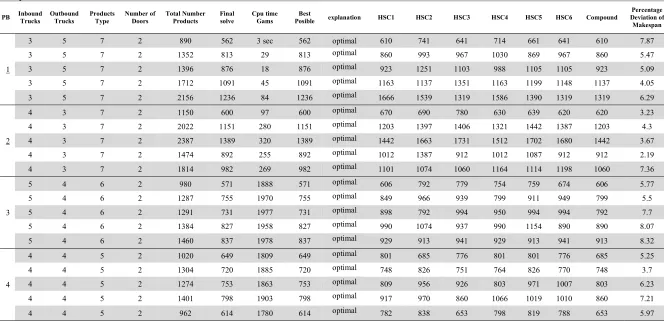
algorithm solved these 20 test sets, and the results are presented in the same table. These problems were used to evaluate the performance of the mathematical models. We also evaluated the performance of the heuristic algorithm and compared the results. Accordingly, numerical tests were applied to evaluate performance in Table 1. As seen in Table 1, the minimum deviation as compared to the optimal software response is 2.19%, and the maximum is 11.34%.

The second test includes problems in a larger size. Results regarding their performance are presented in Table 2. As it can be seen in Table 2, in instance number five, a total number of the sequence are equal to (m!)×(n!)×(q!)×(u!)=6!×5!×4!×3! =12441600 that shows the problem is NP-HARD. Based on the results of evaluating the mathematical model, we realized that as the problem size increases, the software is no longer capable of solving these problems.

Consequently, the software was given the 2000s with smaller sizes to solve the respective problems. Finally, test problems were in the largest size that could be solved by GAMS, but responses provided in the 2000s were not optimum. It is also noteworthy that the heuristic algorithm provided results in less than 10s. Results of Table 2 include the optimal response presented by GAMS as well as a heuristic algorithm. In addition, the deviation percentage of results obtained from the best heuristic algorithm or optimal software result is reported in Table 2. The heuristic algorithm was also executed by MATLAB programming language and by a computer with the processing power of 2.4GHz Intel Core i7 and 6GB RAM.

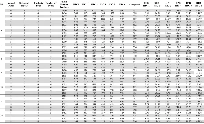
In the next step, we solved problems which could not be solved by GAMS. In this section, 40 problems were generated. The performance index used for comparing the algorithm results isRelative Percentage Difference (RPD). In calculating this index, each problem was solved by a heuristic algorithm with six SC. Since the target function value was different for each problem, it could not be directly compared. Hence, the relative deviation percentage was applied for problem-solving. After solving all problems for each size, the best response obtained for each problem (i.e. the least makespan.) was computed as Minsol.

Then, the relative deviation percentage was computed by the following formula. Results are presented in Table 2.

100

sol sol

sol

Alg Min RPD

Min



  (26)

To obtain more accurate results, ANOVA was also used. Regression analysis was done, i.e. analyzing and modeling the relationship between a response variable and one or more independent variables. It differs from the regression in two terms: 1) independent variables are qualitative (classified), and 2) there is no assumption about the nature of the relationship. That is, the model does not guarantee any indices for variables.

ANOVA is applied to compare group means. To do so, we consider H0 and H1. H0 represents equal means

between more than two groups. H1 represents the constraint of at least one of them with others. Based on

H0, the respective factor does not create a significant difference between the mean and distribution place

of data. When H0 is rejected (and, as a result, H1 is approved), it can be concluded that the respective

factor is effective and can create a significant difference between the least mean of a group and other groups (Tables 3 and 4).

(15)

[image:15.792.74.738.92.413.2]

Table 1

Examples results in small size

PB Inbound _Trucks Outbound _Trucks Products _Type Number of _Doors Total Number _Products Final _solve Cpu time_Gams _PosibleBest explanation HSC1 HSC2 HSC3 HSC4 HSC5 HSC6 Compound Deviation of Percentage Makespan

1

3 5 7 2 890 562 3 sec 562 optimal 610 741 641 714 661 641 610 7.87

3 5 7 2 1352 813 29 813 optimal 860 993 967 1030 869 967 860 5.47

3 5 7 2 1396 876 18 876 optimal 923 1251 1103 988 1105 1105 923 5.09

3 5 7 2 1712 1091 45 1091 optimal 1163 1137 1351 1163 1199 1148 1137 4.05

3 5 7 2 2156 1236 84 1236 optimal 1666 1539 1319 1586 1390 1319 1319 6.29

2

4 3 7 2 1150 600 97 600 optimal 670 690 780 630 639 620 620 3.23

4 3 7 2 2022 1151 280 1151 optimal 1203 1397 1406 1321 1442 1387 1203 4.3

4 3 7 2 2387 1389 320 1389 optimal 1442 1663 1731 1512 1702 1680 1442 3.67

4 3 7 2 1474 892 255 892 optimal 1012 1387 912 1012 1087 912 912 2.19

4 3 7 2 1814 982 269 982 optimal 1101 1074 1060 1164 1114 1198 1060 7.36

3

5 4 6 2 980 571 1888 571 optimal 606 792 779 754 759 674 606 5.77

5 4 6 2 1287 755 1970 755 optimal 849 966 939 799 911 949 799 5.5

5 4 6 2 1291 731 1977 731 optimal 898 792 994 950 994 994 792 7.7

5 4 6 2 1384 827 1958 827 optimal 990 1074 937 990 1154 890 890 8.07

5 4 6 2 1460 837 1978 837 optimal 929 913 941 929 913 941 913 8.32

4

4 4 5 2 1020 649 1809 649 optimal 801 685 776 801 801 776 685 5.25

4 4 5 2 1304 720 1885 720 optimal 748 826 751 764 826 770 748 3.7

4 4 5 2 1274 753 1863 753 optimal 809 956 926 803 971 1007 803 6.23

4 4 5 2 1401 798 1903 798 optimal 917 970 860 1066 1019 1010 860 7.21

(16)

[image:16.792.72.743.112.520.2]

Table 2

Examples results in large size

PB Inbound _Trucks Outbound _Trucks Products _Type Number of _Doors Number Total

Products HSC1 HSC 2 HSC 3 HSC 4 HSC 5 HSC 6 Compound RPD

HSC 1 HSC 2 RPD HSC 3 RPD HSC 4 RPD HSC 5 RPD HSC 6 RPD

5

6 5 4 3 2030 932 990 1123 1155 1340 1361 932 0.00 6.22 20.49 23.93 43.78 46.03 6 5 4 3 1456 749 815 698 749 1127 866 698 6.81 16.76 0.00 7.31 61.46 24.07 6 5 4 3 1697 1141 952 789 1003 900 692 692 39.35 37.57 14.02 44.94 30.06 0.00 6 5 4 3 1549 959 780 949 1122 858 989 780 18.67 0.00 21.67 43.85 10.00 26.79 6 5 4 3 1246 642 794 720 776 813 778 642 0.00 23.68 12.15 20.87 26.64 21.18

6

5 5 5 3 1033 502 643 530 526 681 519 502 0.00 28.09 5.58 4.78 35.66 3.39 5 5 5 3 2128 912 1070 1049 1168 1231 1190 912 0.00 17.32 15.02 28.07 34.98 30.48 5 5 5 3 1574 863 1051 897 804 1018 1148 804 6.84 30.72 11.57 0.00 26.62 42.79 5 5 5 3 1122 509 572 655 711 683 679 509 0.00 12.38 28.68 39.69 34.18 33.40 5 5 5 3 1489 787 973 707 798 1053 993 707 10.17 37.62 0.00 12.87 48.94 40.45

7

5 6 4 4 1371 700 596 559 738 620 752 559 20.14 6.62 0.00 32.02 10.91 34.53 5 6 4 4 1399 729 595 698 725 629 707 595 18.38 0.00 17.31 21.85 5.71 18.82 5 6 4 4 1151 473 591 515 412 593 515 412 12.90 43.45 25.00 0.00 43.93 25.00 5 6 4 4 1312 601 699 600 605 536 618 536 10.82 30.41 11.94 12.87 0.00 15.30 5 6 4 4 1226 530 559 606 544 520 585 520 1.89 7.50 16.54 4.62 0.00 12.50

8

6 6 6 4 1703 657 794 801 912 756 797 657 0.00 20.85 21.92 38.81 15.07 21.31 6 6 6 4 1848 810 841 847 851 993 1010 810 0.00 3.83 4.57 5.06 22.59 24.69 6 6 6 4 1912 766 790 856 607 700 836 607 20.76 30.15 41.02 0.00 15.32 37.73 6 6 6 4 2069 648 843 960 648 919 1120 648 0.00 30.09 48.15 0.00 41.82 72.84 6 6 6 4 1599 696 972 873 627 827 895 627 9.91 55.02 39.23 0.00 31.90 42.74

9

6 7 4 4 1563 568 854 733 636 759 729 568 0.00 50.35 29.05 11.97 33.63 28.35 6 7 4 4 1620 695 834 770 709 1090 804 695 0.00 20.00 10.79 2.01 56.83 15.68 6 7 4 4 1402 514 651 591 529 539 726 514 0.00 26.65 14.98 2.92 4.86 41.25 6 7 4 4 1695 628 730 541 676 797 667 541 13.85 34.94 0.00 24.95 47.32 23.29 6 7 4 4 1798 654 870 746 825 865 900 654 0.00 33.03 14.07 26.15 32.26 37.61

10

7 7 4 4 2623 813 1122 1153 798 1220 1145 798 1.85 40.60 44.49 0.00 52.88 43.48 7 7 4 4 1785 705 795 675 639 869 652 639 9.36 24.41 5.63 0.00 35.99 2.03 7 7 4 4 1946 712 958 883 723 791 933 712 0.00 34.55 24.02 1.54 11.10 31.04 7 7 4 4 1617 700 764 830 794 998 867 700 0.00 9.14 18.57 13.43 42.57 23.86 7 7 4 4 1505 710 892 727 693 845 935 693 2.39 28.72 4.91 0.00 21.93 34.92

11

8 7 4 4 1658 674 851 803 812 953 793 674 0.00 26.26 19.14 20.47 41.39 17.66 8 7 4 4 1911 779 918 799 687 861 903 687 11.81 33.62 16.30 0.00 25.33 31.44 8 7 4 4 1275 487 709 743 523 702 662 487 0.00 45.59 52.57 7.39 44.15 35.93 8 7 4 4 1311 504 564 543 490 699 673 490 2.78 15.10 10.82 0.00 42.65 37.35 8 7 4 4 1741 637 801 660 795 823 676 637 0.00 25.75 3.61 24.80 29.20 6.12

12

(17)

[image:17.612.65.530.70.113.2]

Table 3

ANOVA results

Source DF SS MS F P

Algorithm 5 19591 3918 20.10 0.000

Error 234 45605 195

[image:17.612.68.531.144.211.2]

Total 239 65196

Table 4

Individual 95% CIs For Mean Based on Pooled StDev and grouping Information

Table 5

Fisher 90% Individual confidence intervals all pairwise comparisons

Algorithms Lower Center Upper

HSC1 and HSC2 13.36 18.52 23.67

HSC1 and HSC3 7.24 12.39 17.55

HSC1 and HSC4 1.15 6.31 11.46

HSC1 and HSC5 18.55 23.70 28.86

HSC1 and HSC6 19.71 24.86 30.02

HSC2 and HSC3 -11.28 -6.12 -0.97

HSC2 and HSC4 -17.37 -12.21 -7.06

HSC2 and HSC5 0.03 5.18 10.34

HSC2 and HSC6 1.19 6.34 11.50

HSC3 and HSC4 -11.24 -6.09 -0.93

HSC3 and HSC5 6.15 11.31 16.46

HSC3 and HSC6 7.31 12.47 17.62

HSC4 and HSC5 12.24 17.39 22.55

HSC4 and HSC6 13.40 18.55 23.71

HSC5 and HSC6 -4.00 1.16 6.31

Based on the results of the algorithms, we found that P-value<α in Table 3. Hence, H0 representing equal

samples’ means is rejected. We used the Least Significant Difference (LSD) for further examination. This method is applied to the paired comparison of factor levels’ means. As compared to other methods, the advantage of this method is that it includes all states. First, we conducted LSD calculations and the paired comparison of algorithms.

, 2

1 1

6.18 N a

i j

LSD t MSE

n n

 _

 

  _  _

 

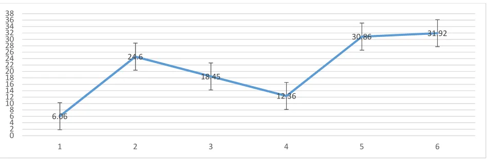
Before determining LSD, the diagram of means’ heuristic algorithms with six SC is displayed in Fig. 2.

Fig. 2. Means comparison

6.06

24.6

18.45

12.36

30.86 31.92

0 2 4 6 8 10 12 14 16 18 20 22 24 26 28 30 32 34 36 38

1 2 3 4 5 6

Level N Mean StDev Grouping

HSC1 40 6.06 8.49 A

HSC2 40 24.67 13.76 D

HSC3 40 18.45 14.19 C

HSC4 40 12.36 13.92 B

HSC5 40 30.86 16.04 E

[image:17.612.65.537.240.400.2] [image:17.612.67.541.542.698.2]

(18)

This diagram shows the mean difference in the heuristic algorithm.

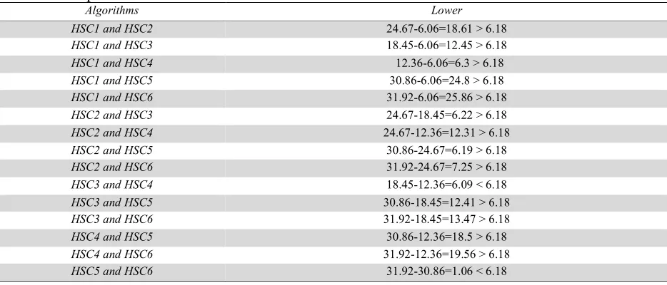
[image:18.612.67.534.136.336.2]

Now, we conduct a paired comparison. According to the results in Table 6, SC1 is the best compared to other SCs, and after that, SC4 is better than the others.

Table 6

APaired comparison

Algorithms Lower

HSC1 and HSC2 24.67-6.06=18.61 > 6.18

HSC1 and HSC3 18.45-6.06=12.45 > 6.18

HSC1 and HSC4 12.36-6.06=6.3 > 6.18

HSC1 and HSC5 30.86-6.06=24.8 > 6.18

HSC1 and HSC6 31.92-6.06=25.86 > 6.18

HSC2 and HSC3 24.67-18.45=6.22 > 6.18

HSC2 and HSC4 24.67-12.36=12.31 > 6.18

HSC2 and HSC5 30.86-24.67=6.19 > 6.18

HSC2 and HSC6 31.92-24.67=7.25 > 6.18

HSC3 and HSC4 18.45-12.36=6.09 < 6.18

HSC3 and HSC5 30.86-18.45=12.41 > 6.18

HSC3 and HSC6 31.92-18.45=13.47 > 6.18

HSC4 and HSC5 30.86-12.36=18.5 > 6.18

HSC4 and HSC6 31.92-12.36=19.56 > 6.18

HSC5 and HSC6 31.92-30.86=1.06 < 6.18

6. Conclusion and future research

This paper has considered truck-to-door sequencing with repeat truck holding pattern in a multi-door cross-docking system. The most important feature of this paper is to consider a repeat truck holding pattern in truck-to-door sequencing, and it is the first study that uses repeat truck holding pattern in solving truck-to-door sequencing problems. One of the ways to increase the stability of cross-dock planning against disruptions and uncertainty is repeat truck holding the pattern in inbound trucks to save time for unloading so the outbound trucks can leave the outbound doors on time, but in this study, we only considered repeat truck holding pattern without consideration of uncertainty in arrival time. This study is a basic model in this area. The objective of the presented model was to identify the proper sequence of inbound and outbound trucks in a multi-door cross-dock center and to assign the products simultaneously to minimize the total completion time. Overall, the heuristic algorithm with SC1 and SC4 compared with other SCs are in better condition and provide better solutions in most test problems. On average, the solutions are within 5.66 % away from the optimal solution. The percentage deviation from optimal solutions ranged from 2.19% to 8.32%. For future research, considering the uncertainties in arrival time, unloading time, and facility breakdown inside the cross-dock center can help simulate the real environment. In addition, an integrated model can be developed to consider the internal and external processes together. Finally, the presented heuristic can be improved in terms of finding the nearest results to the optimal solution.

References

Boloori Arabani, A. R., Fatemi Ghomi, S. M. T., & Zandieh, M. (2011). Meta-heuristics implementation for scheduling of trucks in a cross-docking system with temporary storage. Expert Systems with Applications, 38(3), 1964-1979.

(19)

Cóccola, M., Méndez, C. A., & Dondo, R. G. (2015). A branch-and-price approach to evaluate the role of cross-docking operations in consolidated supply chains. Computers & Chemical Engineering, 80, 15-29.

Dondo, R., & Cerdá, J. (2013). A sweep-heuristic based formulation for the vehicle routing problem with cross-docking. Computers & Chemical Engineering, 48, 293-311.

Dondo, R., & Cerdá, J. (2014). A monolithic approach to vehicle routing and operations scheduling of a cross-dock system with multiple dock doors. Computers & Chemical Engineering, 63, 184-205. Fazel Zarandi, M. H., Khorshidian, H., & Akbarpour Shirazi, M. (2016). A constraint programming

model for the scheduling of JIT cross-docking systems with preemption. Journal of Intelligent Manufacturing, 27(2), 297-313.

Konur, D., & Golias, M. M. (2013). Analysis of different approaches to cross-dock truck scheduling with truck arrival time uncertainty. Computers & Industrial Engineering, 65(4), 663-672.

Kuo, Y. (2013). Optimizing truck sequencing and truck dock assignment in a cross docking system.

Expert Systems with Applications, 40(14), 5532-5541.

Ladier, A.-L., & Alpan, G. (2016). Cross-docking operations: Current research versus industry practice.

Omega, 62, 145-162.

Larbi, R., Alpan, G., & Penz, B. (2009). Scheduling transshipment operations in a multiple inbound and outbound door crossdock. Paper presented at the Computers & Industrial Engineering, 2009. CIE 2009. International Conference on.

Li, Y., Lim, A., & Rodrigues, B. (2004). Crossdocking—JIT scheduling with time windows. Journal of the Operational Research Society, 55(12), 1342-1351.

Liao, T. W., Egbelu, P. J., & Chang, P. C. (2012). Two hybrid differential evolution algorithms for optimal inbound and outbound truck sequencing in cross docking operations. Applied Soft Computing, 12(11), 3683-3697.

Lim, A., Ma, H., & Miao, Z. (2006). Truck Dock Assignment Problem with Time Windows and Capacity Constraint in Transshipment Network Through Crossdocks, Berlin, Heidelberg.

Madani-Isfahani, M., Tavakkoli-Moghaddam, R., & Naderi, B. (2014). Multiple cross-docks scheduling using two meta-heuristic algorithms. Computers & Industrial Engineering, 74, 129-138. doi: https://doi.org/10.1016/j.cie.2014.05.009

Maknoon, M. Y., & Baptiste, P. (2009). Cross-docking: increasing platform efficiency by sequencing incoming and outgoing semi-trailers. International Journal of Logistics Research and Applications, 12(4), 249-261.

McWilliams, D.L. (2005, 4-7 Dec. 2005). Simulation-based scheduling for parcel consolidation terminals: a comparison of iterative improvement and simulated annealing. Paper presented at the Proceedings of the Winter Simulation Conference, 2005.

McWilliams, D.L. (2009). Genetic-based scheduling to solve the parcel hub scheduling problem.

Computers & Industrial Engineering, 56(4), 1607-1616.

McWilliams, D.L. (2010). Iterative improvement to solve the parcel hub scheduling problem. Computers & Industrial Engineering, 59(1), 136-144.

McWilliams, D. L. (2009). A dynamic load-balancing scheme for the parcel hub-scheduling problem.

McWilliams, D. L., Stanfield, P. M., & Geiger, C. D. (2005). The parcel hub scheduling problem: A

simulation-based solution approach. Computers & Industrial Engineering, 49(3), 393-412.

McWilliams., Stanfield, P. M., & Geiger, C. D. (2008). Minimizing the completion time of the transfer operations in a central parcel consolidation terminal with unequal-batch-size inbound trailers.

Miao, Z., Lim, A., & Ma, H. (2009). Truck dock assignment problem with operational time constraint within crossdocks. European Journal of Operational Research, 192(1), 105-115.

(20)

Nassief, W., Contreras, I., & As’ad, R. (2016). A mixed-integer programming formulation and Lagrangean relaxation for the cross-dock door assignment problem. International Journal of Production Research, 54(2), 494-508.

Shahin Moghadam, S., Fatemi Ghomi, S. M. T., & Karimi, B. (2014). Vehicle routing scheduling problem with cross docking and split deliveries. Computers & Chemical Engineering, 69, 98-107. Van Belle, J., Valckenaers, P., & Cattrysse, D. (2012). Cross-docking: State of the art. Omega, 40(6),

827-846.

Wisittipanich, W., & Hengmeechai, P. (2017). Truck scheduling in multi-door cross docking terminal by modified particle swarm optimization. Computers & Industrial Engineering, 113, 793-802.

Yazdani, M., Naderi, B., & Mousakhani, M. (2015). A Model and Metaheuristic for Truck Scheduling in Multi-door Cross-dock Problems. Intelligent Automation & Soft Computing, 21(4), 633-644. Ye, Y., Li, J., Li, K., & Fu, H. (2018). Cross-docking truck scheduling with product unloading/loading

constraints based on an improved particle swarm optimisation algorithm. International Journal of Production Research, 1-21. doi: 10.1080/00207543.2018.1464678

Yu, W. (2002). Operational strategies for cross docking systems. (Retrospective Theses and Dissertations. 413. ).

Yu, W., & Egbelu, P. J. (2008). Scheduling of inbound and outbound trucks in cross docking systems with temporary storage. European Journal of Operational Research, 184(1), 377-396.