9614
|
www.ecolevol.org Ecology and Evolution. 2018;8:9614–9623.1
|
INTRODUCTION
Complex systems are constantly adapting through interactions among components, with feedback loops that can generate system- level behaviors that are not simply the sum of the parts (Levin, 1998).
Accordingly, the dynamics of complex systems are difficult to pre-dict using reductionist- based models. Despite the variability within complex systems, there exist system- level properties that are more stable than the individual components that comprise them. Coupled nonlinear interactions can create positive feedback loops over Received: 11 June 2017
|
Revised: 4 May 2018|
Accepted: 20 May 2018DOI: 10.1002/ece3.4297
O R I G I N A L R E S E A R C H
A method to detect discontinuities in census data
Chris Barichievy
1,2|
David G. Angeler
3|
Tarsha Eason
4|
Ahjond S. Garmestani
4|
Kirsty L. Nash
5,6|
Craig A. Stow
7|
Shana Sundstrom
8|
Craig R. Allen
9This is an open access article under the terms of the Creative Commons Attribution License, which permits use, distribution and reproduction in any medium, provided the original work is properly cited.
© 2018 The Authors. Ecology and Evolution published by John Wiley & Sons Ltd. 1Zoological Society of London, London, UK
2Institute for Communities and Wildlife in
Africa, University of Cape Town, Cape Town, South Africa
3Department of Aquatic Sciences and
Assessment, Swedish University of Agricultural Sciences, Uppsala, Sweden 4U.S. Environmental Protection Agency, Office of Research and Development, National Risk Management Research Laboratory, Cincinnati, Ohio 5Centre for Marine Socioecology, Hobart, TAS, Australia
6Institute for Marine and Antarctic
Studies, University of Tasmania, Hobart, TAS, Australia
7NOAA Great Lakes Environmental Research
Laboratory, Ann Arbor, Michigan
8School of Natural Resources, University of Nebraska, Lincoln, Nebraska
9U.S. Geological Survey, Nebraska Cooperative Fish and Wildlife Research Unit, University of Nebraska, Lincoln, Nebraska
Correspondence
Chris Barichievy, Zoological Society of London, Regents Park, London, UK Email: [email protected]
Funding information
United States Geological Survey; Nebraska Game and Parks Commission; University of Nebraska Lincoln; United States Fish and Wildlife Service; Wildlife Management Institute
Abstract
The distribution of pattern across scales has predictive power in the analysis of com-plex systems. Discontinuity approaches remain a fruitful avenue of research in the quest for quantitative measures of resilience because discontinuity analysis provides an objective means of identifying scales in complex systems and facilitates delinea-tion of hierarchical patterns in processes, structure, and resources. However, current discontinuity methods have been considered too subjective, too complicated and opaque, or have become computationally obsolete; given the ubiquity of discontinui-ties in ecological and other complex systems, a simple and transparent method for detection is needed. In this study, we present a method to detect discontinuities in census data based on resampling of a neutral model and provide the R code used to run the analyses. This method has the potential for advancing basic and applied eco-logical research.
K E Y W O R D S
relatively discrete spatial and temporal scales. These “self- reinforcing assembly states” (Stallins, 2006) are variously described as: “attrac-tors” (Baas, 2002; Harrison, Massey, & Richards, 2006; Thompson et al., 2001), “stability domains” (Gunderson, 2000) or “domains of scale” (Wiens, 1989) or “scales of opportunity” (Garmestani, Allen, & Gunderson, 2009). Nevertheless, all of these terms refer to specific spatial or temporal windows within which pattern and process are tightly coupled relative to the other scales of the system. The result is a limited set of frequencies in both space and time at which dom-inant patterns and processes operate, reflected as the discontinu-ous distribution of pattern when compared across scales of analysis (Figure 1). Analyzing the dynamics of the cross- scale pattern over space and time allows inference about changes in a system’s relative resilience and other system properties (Allen & Holling, 2008).
Much of the discontinuity literature is based on the examination of body mass distributions because the scale at which an organism perceives the environment and procures resources is a function of its size (Calder, 1984). The body mass of an animal is an integrated measure of selective pressures affecting the evolution of a species and is highly allometric with many life history traits (Peters 1983). Organism body size affects speed and distance of travel (Harestad & Bunnel, 1979), processing of food, thermoregulation, physical structure, and the required quantity and aggregation of resources (Peterson, Allen, & Holling, 1998). Resources and habitat structure are not evenly distributed across the landscape; rather their avail-ability varies among spatial and temporal scales (Wiens, 1989). Heterogeneously distributed resources across scales generate mul-timodal body size distributions, which is evidence of a discontinu-ity. Species are clustered at scales where resources are available and separated from neighboring body size aggregations by discon-tinuities corresponding to scales where resources are limited or highly variable in space and time (Nash, Allen, Angeler et al., 2014). Researchers have argued that discontinuities are a signature of hi-erarchical complex adaptive systems (Holling, 1992) and have been
identified in ecological and other complex systems, including city and firm size distributions and economic data (Garmestani, Allen, & Bessey, 2005; Garmestani, Allen, Mittelstaedt, Stow, & Ward, 2006; Sundstrom, Angeler, Garmestani, García, & Allen, 2014).
Discontinuity research has direct application to ecosystem man-agement (Angeler et al., 2016). Because discontinuity analyses ob-jectively identify the scales at which pattern and process manifest, it is possible to examine the relationship between these scales and system features such as ecological resilience (Allen, Gunderson, & Johnson, 2005; Angeler, Allen, & Johnson, 2012; Baho et al., 2015; Stow, Allen, & Garmestani, 2007; Sundstrom, Allen, & Barichievy, 2012), invasion and extinction risk (Allen, 2006; Allen et al., 2005; Angeler et al., 2012; Raffaelli, Hardiman, Smart, Yamanaka, & White, 2016), and as an early warning signal of a regime shift (Spanbauer et al., 2016). For example, ecological resilience emerges in part from the distribution of ecological functions as provided by species. When a system has a high diversity of functions within each scale and a high redundancy of function across scales, it is better able to buffer disturbances (Peterson et al., 1998; Scheffer et al., 2015). Similarly, species with body sizes that place them close to a discon-tinuity are more likely to successfully invade a new ecosystem, or alternatively, are more likely to be driven to extinction (Allen, 2006; Allen et al., 2005; Angeler et al., 2012). Finally, identifying the prox-imity of a system to a regime shift is a fundamental goal in systems ecology, and it has been demonstrated that the number and location of discontinuities in community body size distributions are highly conservative through time, so significant shifts in the discontinuous distributions serve as an early warning signal of an impending sys-tem regime shift (Spanbauer et al., 2016).
1.1
|
Methods available for discontinuity analysis
Numerous methods have been used to identify discontinuities in datasets (Skillen & Maurer, 2008). In general, these methodscompare the difference between adjacent ranked observations, for instance, the difference in body mass size between rank- ordered species (Allen et al., 2005; Holling, 1992; Siemann & Brown, 1999; Stow et al., 2007). Early discontinuity research utilized a body mass difference index, in which differences between rank- ordered body masses were compared, and a discontinuity was defined as a dif-ference between two values that were greater than specified cri-terion. Relative measures were needed because direct comparisons between absolute values of ranked body masses are not meaningful. For example, a five- gram difference between two shrew species is more meaningful than a five- gram difference between deer species, simply because of the size of the animals, thus, a scaling exponent or log transformation was used. Another option was subjective transformations (Holling, 1992) in which bird body masses were transformed by 1.3 and mammals by 1.1, and a difference index was calculated as HI = (M(n+1)−M(n−1))/M(n))γ, where M is the mean body
mass of the species index n in a fully censused community (Restrepo, Renjifo, & Marples, 1997). Alternatively, Siemann and Brown (1999) log- transformed the data, and the difference was calculated as SB = log10((M(n+1))/(M(n))). Although informative, these difference index methods suffer from inherent subjectivity.
Various resampling methods were developed to detect disconti-nuities more objectively. The Discontinuity Index developed by Stow et al. (2007) tested the vector norm of the observed data against a population of hypothetical Discontinuity Index values. The hypo-thetical population was created by resampling a hypohypo-thetical null distribution of uniform distances with the same sample size as the observed dataset. The result is a single value describing the proba-bility that the Discontinuity Index of the dataset is higher than that created randomly. Straightforward and robust, the Discontinuity Index (Stow et al., 2007) is useful as a general metric describing the dataset but does not identify where the discontinuities are located along the rank- ordered axis.
The Gap Rarity Index (GRI) (Restrepo et al., 1997) utilized a neu-tral null model that was repeatedly sampled as: gap(n) = log10(M(n+1))− log10(M(n)), where M is the mean body mass of the species n in a fully censused community. The resampling creates a hypothetical distribution of gaps against which the gaps within the real data are tested. The GRI has been the most widely used method to date in discontinuity analysis of census data (Nash, Allen, Baricjievy et al., 2014; Sundstrom et al., 2012; Wardwell 2008) and is preferred due to its simplicity of inference. The GRI uses a neutral model, based on a standard kernel density estimator, that is generated to approx-imate a unimodal continuous distribution and is used to analyze for evidence of multimodality (Silverman, 1981). Practically, this sets up a null hypothesis against which the real data are compared to test for departure from some form of central tendency, which is expected from equilibrium systems (viz. Allen, Forys, & Holling, 1999; Forys & Allen, 2002). Discontinuities are defined as areas between suc-cessive, ranked body masses significantly exceeding that generated by the continuous null distribution. This test for departure is carried out using a resampling approach, which allows for robust compar-ison, incorporates the effects of sample size, and accounts for the
associated uncertainty of whether a discontinuity is real or simply a sampling artifact. However, the major limitation of the GRI algorithm is that it uses arbitrary constants which are not a dataset- specific es-timate, but rather a constant used in the original programming which has unclear biological origins and so cannot be rigorously applied across different types of complex systems.
Other statistical approaches are hierarchical cluster analysis (HCA) and classification and regression trees (CART), including the Bayesian version thereof (Chipman, George, & McCulloch, 1998). These three methods use various algorithms to find the “best” clus-tering based on minimizing a cost function. BCART is notably the most reliable method, where the tree generating algorithm min-imizes within- group entropy, which is consistent with the premise of the discontinuity theory. BCART is relatively robust to variations in tuning, provides repeatable results, and was used successfully to show regime shifts in paleo- diatom community assemblages (Spanbauer et al., 2016) and the resilience of plankton communities at macroecological scale (Baho et al., 2015).
HCA, CART, and BCART are optimal for clustering and classifi-cation of large multivariate datasets; however, these methods are also difficult to interpret in the context of discontinuity analyses. The algorithms essentially partition variance and are not testing any hypothesis or null model. They are useful in partitioning data into subpopulations of data with latent variables; however, we are uti-lizing univariate data where the datum is a proxy for the scale of pattern and process. Therefore, there is no ecologically meaningful inference that can be made on the results of variance partitioning methods, and so the “significance” of a cluster of body masses is difficult to understand. Stow et al. (2007) have advocated finding consensus using multiple methods. The determination of what con-stitutes a significant cluster will always be a challenge and remains a contentious issue when identifying the location of discontinuities. Thus, there is a need for a contemporary, intuitive method to detect discontinuities from census data. We present here an application that compares the observed distribution with that generated from a neutral null, formulated from a Gaussian distribution. We then uti-lize a bootstrapping approach to test to compare the observed data versus that generated from the neutral null to quantitatively assess the likelihood that differences between body masses are generated randomly, or are likely to represent a discontinuity. Although most closely aligned to the GRI as an approach to discontinuity analysis, the method presented here is novel in that it does not utilize any fixed conversion or tuning parameters and therefore can be used across multiple systems in which the user may want to test for dis-continuities; it is intuitive to understand the outputs; and it will be publicly available as an R script to allow straightforward application across studies.
2
|
METHODS
approach that compares rank- ordered differences in data to differ-ences generated through resampling the neutral null. We then com-pare the observed data to the bootstrapped samples and calculate the percentile of the bootstrap distribution to infer the likelihood that the gap is not through random chance.
2.1
|
Data requirements
The DD is designed for census data, as opposed to sample data. We use body size as an example, but researchers working in other types of complex systems have chosen proxies that represent an integration of system- specific drivers, such as firm size or city size (Sundstrom et al., 2014) and biomass (Angeler et al., 2012). Abundance measures are not required, just presence data such as the bird or mammal species assemblages found in boreal forests, grasslands, and arid areas as found in Holling (1992). Although our method may be appropriate for determinate growth species, further research is required for indeterminate growth species such as fishes (Nash, Allen, Barichievy et al., 2014).
2.2
|
The neutral null
Kernel density estimates of log10-transformed data (m) are gener-ated for bandwidth values (h) ranging from 0 to half of the range in the dataset. We used half of the range as this avoids too many edge effects being introduced by the smoothing function and makes the computation more efficient; however, this can be changed if neces-sary by the user. A lower bound of zero was used as body masses can only be positive so it is not sensible to generate a model that predicts negative body mass. We utilized a bandwidth increment of 0.001 (i.e., h(j + 1) = h(j) + 0.001 for j = 1… n). The estimates are eas-ily calculated in R using the base package and the density function (Equation 1 and 2), with the bandwidth bounded to be greater than 0 (0 < h<∞).
where K is the standard normal density function
and h is the bandwidth at index j, against which the masses of vector
m, at index i are calculated. A kernel density estimator generates, for a given bandwidth, a smoothed curve that integrates to 1, which shows the “density” of data points at the particular value.
The output is a set of smoothed kernel density functions of vary-ing bandwidths rangvary-ing from 0 to half of the data range. For each of these kernel density estimates, the second derivative test is uti-lized to determine whether the function is unimodal. The neutral null model is selected as the kernel density estimate with the smallest bandwidth that is unimodal.
We have used the Gaussian function as the smoothing function as it speaks to the common ecological expectation that there is a
limited range of scales of resource distribution, implying an optimum scale at which an animal can exploit resources. For instance, in the absence of reinforcing process rates, we would not expect multiple scales or hierarchical pattern and process. Instead, an equilibrium of pattern and process would be reached (Wu & Loucks, 1995) which would manifest as processes being distributed over a continuous, unimodal distribution within the bounds of realistic system scales. There may be utility in having a uniform distribution as a neutral null model, but the ecological implication of a uniform distribution is that there is no optimum scale at which pattern is more or less likely to occur. Currently, the ecological meaning behind using a uni-form distribution as a null hypothesis is not evident, but the method presented does allow for user- defined neutral nulls to be generated and tested.
2.3
|
Resampling and calculating the percentile
The neutral null represents a null hypothesis of an “optimal” body size for a given system. This neutral model is redrawn without re-placement (we used 5,000 times), with the same sample size as the observed data. For instance, if there are 60 species in the commu-nity, a sample size of 60 is resampled without replacement 5,000 times. For each draw, the sampled data are rank- ordered and the dif-ferences between each of the rank- ordered, simulated body masses are calculated. By doing this multiple times, a distribution of gap sizes is generated for each rank- ordered gap. Each of the observed differences is compared to the resampled distribution of the same rank, and the percentile (the value below which a given percentage of observations in a group of observations fall) of the resampled gap distribution is calculated. The gap percentile is then used as a meas-ure of how likely the observed difference between census points is to those which can be considered randomly sampled from the neutral null distribution. Decisions regarding what percentile to ac-cept as a gap are akin to alpha value assessment in any frequentist method, and inference can be made accordingly.2.4
|
Comparison of existing methods
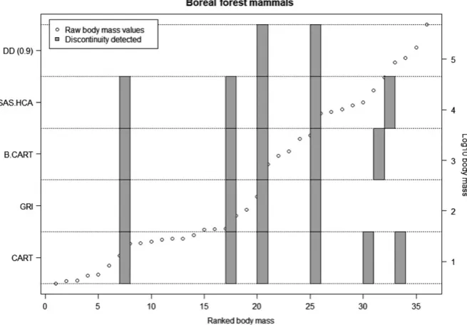
To illustrate whether the DD algorithm presented here is consist-ent with the methods used in the discontinuity literature, we com-pared the outputs of the DD algorithm to those from the GRI, CART, BCART, and HCA for datasets previously published in discontinuity studies. These datasets are body mass distributions for boreal forest mammals (N = 36), boreal forest birds (N = 101), boreal prairie mam-mals (N = 53), boreal prairie birds (N = 108) (raw data, including home ranges, are available in Holling, 1992), as well as Kalahari mammals and fynbos birds (Allen, 1997).
2.5
|
Sensitivity analysis
The DD must be robust to common research challenges of realistic census sizes (number of species in a community), and the method must be verified for incomplete census data (sample data). We (1)
̂
f(hj)(m)= 1
nhj ∑n
(i=1)
K (m
−mi hj
)
,
(2)
K(x)=e
−12x 2
√
tested three hypotheses: The DD algorithm can reliably detect gaps in data that encompasses (a) multiple scales, (b) under condi-tions of reduced census success, and (c) under condicondi-tions of low species richness.
To approximate realistic ecological scenarios, we simulated a dataset similar in scale and composition to the Holling (1992) bo-real bird body mass dataset from which a species pool of 102 birds yielded ten discontinuities which separated 11 clusters of similarly sized birds. Gaussian mixture models were used to generate data of known multimodal distributions across scales of analysis. The mul-timodal distributions represent the multiple and discrete scale do-mains from which a sample is drawn. For these sensitivity analyses, test data were drawn from a Gaussian mixture model with ten modes with means and variances increasing evenly on a log scale. A hypo-thetical census of 100 data points (simulating species average body masses sampled from a multimodal distribution) was generated with equivalent weights in the mixture.
One thousand test datasets with differing sample sizes and cen-sus success (ability to detect all species in the community) were gen-erated and tested for discontinuities using the DD. This gengen-erated a population of discontinuities from which the effects of sample size and census success could be tested. Because each experimental dataset was an independent simulation, it was necessary to objec-tively cluster discontinuity values together to measure the effect of changing simulation parameters on the location of discontinuities. If the algorithm reruns an analysis on the same dataset, yet the discon-tinuities are identified in different places, the algorithm is not robust, by running repeated analysis of the same dataset we explicitly tested
for this. To do this, the DD was run on all test datasets, and then, independent estimations of discontinuities were clustered together using the mClust package which uses a Bayes clustering algorithm that selects clusters based on the BIC (Bayes information criteria ~ similar to an Akaike information criteria) value was used to deter-mine the best- fit number of clusters. The distribution of disconti-nuities per cluster was then compared under varying conditions of census success and sample size to determine the sensitivity of DD to real- world constraints in the census:
• The population of discontinuities was compared among samples with equal sample size. Sample success was simulated by randomly deleting a proportion of the sampled population. Comparisons were made between proportions sampled from 0.75 to 1. • The population of discontinuities was compared among samples
with unequal sample size. Sample success is assumed to be 1, with sample sizes varying from 20 to 100 samples (increments of 10 values) in the proxy dataset.
3
|
RESULTS
R code for implementing the DD is provided in the Supporting in-formation. The DD method presented in the paper successfully identified known gaps from multimodal mixture models (Figure 2). When comparing the DD results to previous methods (i.e., CART, BCART, HCA, and GRI), we found consistency across many of
the methods. This is evident in both the Boreal foret mammals dataset (Figure 3) and other sample datasets (Figure 4, data from Holling, 1992). The similarity between the GRI and the DD is to be expected, as they are fundamentally similar approaches. Both GRI and DD are more conservative than the variance partition-ing approaches of HCA, CART, and BCART, identifypartition-ing fewer discontinuities.
The method detects discontinuities accurately and precisely under increased sample sizes and census success (Figure 5, top right); however, under relatively lower sample sizes and low census success (Figure 5 bottom left), there is less precision and accuracy in the location of the discontinuities.
4
|
DISCUSSION
The discontinuity detector provides an objective, repeatable method to find discontinuities in census data. This method provides an easy approach for determining scales in research studies which has great utility for complex system- centered research such as predicting in-vasion and extinction, evaluating ecosystem function across scales, and assessing system resilience (Allen & Holling, 2008; Allen et al., 1999, 2005; Sundstrom et al., 2012). The method may, therefore, be useful for addressing management challenges that derive from envi-ronmental change (Angeler et al., 2016).
The DD method presented here improves on the original GRI method by removing a subjective transformation constant, which
makes inference simpler and the method more transparent. The use of the neutral null allows for a hypothesis testing approach as opposed to simply the clustering approach used in alternative methods, which makes for stronger inference around the nature of the discontinuity.
We should also note that while it is unlikely that the method will miss gaps that are in fact real, it is sensitive to detecting er-roneous gaps. Accordingly, interpretation of the results of the DD must be made considering type 2 errors. Overall, the DD algorithm is more conservative than the variance partition methods (HCA, CART, BCART), which is a result of comparing the observed data to a unimodal neutral null (Figure 3). A major challenge in detect-ing discontinuities in census data is that there exists no unambig-uous null model or standard for comparison. Standard statistical procedures arise from trying to make a population- level inference from a (proportionally) small sample. In the investigation of dis-continuities from census data, one is making inference on an ex-tremely small population from a very large (proportional) sample; hence, the concepts from traditional statistical investigations are not fully transferable. We utilize a null hypothesis of a continuous unimodal distribution to simulate a central tendency. The method presented here does allow for varying null models to be used; however, any null model that is used as a basis for comparison can only ever be hypothetical, which opens methodological questions surrounding the null model choice as opposed to the discontinu-ities themselves. Therefore, the ecological meaning behind a uni-form null or skewed null model, for example, would need to be defined prior to the test.
[image:6.595.133.461.50.278.2]How well the census represents what’s in the community and how many species are in a community will affect the precision of the DD in detecting the discontinuities. This is because the variance in the location of the resampled distribution is a function of the number of samples from which the resampling is drawn. If only ten samples are taken from a distribution, the variability in the gaps between in-dividual samples is higher than when there are around 100 samples.
Practically, this may limit the application of the DD for species- poor systems (such as a desert) but, if the census largely accounts for the species in the community, the method will be effective in detecting discontinuities.
The DD method provides a quick, easy to use and, most impor-tantly, transparent method to objectively detect discontinuities in cen-sus data. Such a method will allow for increased discontinuity research F I G U R E 5 Sensitivity analysis of the discontinuity detector algorithm under conditions of varying sample size and sampling success. The
in the various fields of ecology and other complex system science af-fording the ability to build upon this burgeoning area of study.
ACKNOWLEDGMENTS
This research arose from a workshop series, “Understanding and managing for resilience in the face of global change,” which was funded by the USGS John Powell Center for Synthesis and Analysis, and the USGS National Climate Change and Wildlife Center. We thank the Powell Center for supporting collaborative and interdis-ciplinary research efforts. GLERL contribution number 1880. The Nebraska Cooperative Fish and Wildlife Research Unit is jointly supported by a cooperative agreement between the United States Geological Survey, the Nebraska Game and Parks Commission, the University of Nebraska Lincoln, the United States Fish and Wildlife Service, and the Wildlife Management Institute. The views ex-pressed in this article are those of the authors and do not necessarily represent the views or policies of the U.S. Environmental Protection Agency. Any use of trade names is for descriptive purposes only and does not imply endorsement by the U.S. Government.
CONFLIC T OF INTEREST
None declared.
AUTHORS’ CONTRIBUTION
CB was the primary author. CB and KN tested the application. DA, TE, AG, KN, CS, SS, and CA provided development discussion, cri-tique of the method, and contributed significantly to the writing of the manuscript. CA provided the source code for original Neutral Null and obtained permission from the author and helped to develop the theory behind the method.
DATA ACCESSIBILIT Y
All data used are freely available from Holling (1992): Https://esa-journals.onlinelibrary.wiley.com/doi/abs/10.2307/2937313. Source code supplied as Supporting information in this manuscript.
ORCID
Chris Barichievy http://orcid.org/0000-0003-4088-953X
Kirsty L. Nash http://orcid.org/0000-0003-0976-3197
REFERENCES
Allen, C. R. (1997). Scale, Pattern and Process in Biological Invasions.
Dissertation submitted in partial submission for Doctorate of Philosophy. Gainesville, FL: University of Florida
Allen, C. R. (2006). Predictors of introduction success in the South Florida
avifauna. Biological Invasions, 8, 491–500. https://doi.org/10.1007/
s10530-005-6409-x
Allen, C. R., Forys, E. A., & Holling, C. (1999). Body mass patterns predict
invasions and extinctions in transforming landscapes. Ecosystems, 2,
114–121. https://doi.org/10.1007/s100219900063
Allen, C. R., Gunderson, L., & Johnson, A. (2005). The use of disconti-nuities and functional groups to assess relative resilience in
com-plex systems. Ecosystems, 8, 958–966. https://doi.org/10.1007/
s10021-005-0147-x
Allen, C. R., & Holling, C. S. (Eds.). (2008). Discontinuities in ecosystems and other complex systems. New York, NY: University of Columbia Press. 272 pp. https://doi.org/10.7312/alle14444
Angeler, D. G., Allen, C. R., Barichievy, C., Eason, T., Garmestani, A. S., Graham, N. A., … Nash, K. L. (2016). Management applications of
dis-continuity theory. Journal of Applied Ecology, 53, 688–698. https://
doi.org/10.1111/1365-2664.12494
Angeler, D. G., Allen, C. R., & Johnson, R. K. (2012). Insight on inva-sions and resilience derived from spatiotemporal discontinuities of
biomass at local and regional scales. Ecology and Society, 17(2), 32.
http://www.ecologyandsociety.org/vol17/iss2/art32/
Baas, A. C. (2002). Chaos, fractals and self- organization in coastal geomorphology: Simulating dune landscapes in vegetated
envi-ronments. Geomorphology, 48, 309–328. https://doi.org/10.1016/
S0169-555X(02)00187-3
Baho, D., Tavşanoğlu, Ü., Šorf, M., Stefanidis, K., Drakare, S., Scharfenberger, U., … Angeler, D. (2015). Macroecological patterns of resilience revealed through a multinational, synchronized
ex-periment. Sustainability, 7(2), 1142–1160. https://doi.org/10.3390/
su7021142
Calder, W. (1984). Size, function, and life history, Harvard[19] International Commission on Radiological Protection: University Press, London, 1984. Report of the Task Group on Reference Man, Pergamon. Chipman, H. A., George, E. I., & McCulloch, R. E. (1998). Bayesian CART
model search. Journal of American Statistical Association, 93, 935–
948. https://doi.org/10.1080/01621459.1998.10473750
Forys, E. A., & Allen, C. R. (2002). Functional group change within and across scales following invasions and extinctions in the Everglades
ecosystem. Ecosystems, 5, 339–347. https://doi.org/10.1007/
s10021-001-0078-0
Garmestani, A. S., Allen, C. R., & Bessey, K. M. (2005). Time- series analy-sis of clusters in city size distributions. Urban Studies, 42, 1507–1515. https://doi.org/10.1080/00420980500185314
Garmestani, A. S., Allen, C. R., & Gunderson, L. (2009). Panarchy: Discontinuities reveal similarities in the dynamic system structure of
ecological and social systems. Ecology and Society, 14(1), 15. http://
www.ecologyandsociety.org/vol14/iss1/art15/
Garmestani, A. S., Allen, C. R., Mittelstaedt, J. D., Stow, C. A., & Ward, W. A. (2006). Firm size diversity, functional richness, and resilience. Environment and Development Economics, 11, 533–551. https://doi. org/10.1017/S1355770X06003081
Gunderson, L. H. (2000). Ecological resilience–in theory and application. Annual Review of Ecology, Evolution, and Systematics, 42, 5–439. Harestad, A. S., & Bunnel, F. (1979). Home range and body weight–a
re-evaluation. Ecology, 60, 389–402. https://doi.org/10.2307/1937667
Harrison, S., Massey, D., & Richards, K. (2006). Complexity and
emer-gence (another conversation). Area, 38, 465–471. https://doi.
org/10.1111/j.1475-4762.2006.00711.x
Holling, C. S. (1992). Cross- scale morphology, geometry, and
dynam-ics of ecosystems. Ecological Monographs, 62, 447–502. https://doi.
org/10.2307/2937313
Levin, S. A. (1998). Ecosystems and the biosphere as complex
adap-tive systems. Ecosystems, 1, 431–436. https://doi.org/10.1007/
s100219900037
Nash, K. L., Allen, C. R., Angeler, D. G., Barichievy, C., Eason, T., Garmestani, A. S., … Nelson, R. J. (2014). Discontinuities, cross- scale
patterns, and the organization of ecosystems. Ecology, 95, 654–667.
Nash, K. L., Allen, C. R., Barichievy, C., Nyström, M., Sundstrom, S., & Graham, N. A. (2014). Habitat structure and body size distributions: Cross- ecosystem comparison for taxa with determinate and
inde-terminate growth. Oikos, 123, 971–983. https://doi.org/10.1111/
oik.01314
Peterson, G., Allen, C. R., & Holling, C. S. (1998). Ecological resilience,
biodiversity, and scale. Ecosystems, 1, 6–18. https://doi.org/10.1007/
s100219900002
Peters, R. H., & Wassenberg, K. (1983). The effect of body size on animal abundance. Oecologia, 60(1), 89–96.
Raffaelli, D., Hardiman, A., Smart, J., Yamanaka, T., & White, P. C. (2016). The textural discontinuity hypothesis: An exploration at a regional
level. Shortened version: Exploring Holling’s TDH. Oikos, 125, 797–
803. https://doi.org/10.1111/oik.02699
Restrepo, C., Renjifo, L., & Marples, P. (1997). Frugivorous birds in frag-mented neotropical montane forests: landscape pattern and body mass distribution. Trop. For. Remn. Ecol. Manag. Conserv. Fragm. Communities, 171–189.
Scheffer, M., Carpenter, S. R., Dakos, V., & van Nes, E. H. (2015). Generic indicators of ecological resilience: Inferring the chance of a critical
transition. Annual Review of Ecology, Evolution, and Systematics, 46,
145–167.
Siemann, E., & Brown, J. H. (1999). Gaps in mammalian body size
dis-tributions reexamined. Ecology, 80, 2788–2792. https://doi.
org/10.1890/0012-9658(1999)080[2788:GIMBSD]2.0.CO;2 Silverman, B. W. (1981). Using kernel density estimates to
investi-gate multimodality. Journal of the Royal Statistical Society. Series B,
Statistical Methodology, 43(1), 97–99.
Skillen, J. J., & Maurer, B. A. (2008). The ecological significance of discon-tinuities in body-mass distributions. In C. R. Allen & C. Holling (Eds.), Discontinuities in ecosystems and other complex systems (pp. 193–218). New York, NY: Columbia University Press.
Spanbauer, T. L., Allen, C. R., Angeler, D. G., Eason, T., Fritz, S. C., Garmestani, A. S., … Sundstrom, S. M. (2016). Body size distributions signal a regime shift in a lake ecosystem. Presented at the Proc. R. Soc. B, The Royal Society, 20160249.
Stallins, J. A. (2006). Geomorphology and ecology: Unifying themes for
complex systems in biogeomorphology. Geomorphology, 77, 207–216.
https://doi.org/10.1016/j.geomorph.2006.01.005
Stow, C., Allen, C. R., & Garmestani, A. S. (2007). Evaluating discontinu-ities in complex systems: Toward quantitative measures of resilience. Ecology and Society, 12(1), 26. http://www.ecologyandsociety.org/ vol12/iss1/art26/
Sundstrom, S. M., Allen, C. R., & Barichievy, C. (2012). Species, functional
groups, and thresholds in ecological resilience. Conservation Biology,
26, 305–314. https://doi.org/10.1111/j.1523-1739.2011.01822.x
Sundstrom, S. M., Angeler, D. G., Garmestani, A. S., García, J. H., & Allen, C. R. (2014). Transdisciplinary application of cross- scale resilience. Sustainability, 6, 6925–6948. https://doi.org/10.3390/su6106925 Thompson, J. N., Reichman, O., Morin, P. J., Polis, G. A., Power, M. E., Sterner,
R. W., … Hooper, D. U. (2001). Frontiers of Ecology As ecological re-search enters a new era of collaboration, integration, and technological sophistication, four frontiers seem paramount for understanding how biological and physical processes interact over multiple spatial and temporal scales to shape the earth’s biodiversity. BioScience, 51, 15–24. https://doi.org/10.1641/0006-3568(2001)051[0015:FOE]2.0.CO;2 Wardwell, D. A., Allen, C. R., Peterson, G. D., & Tyre, A. J. (2008). A test of
the cross- scale resilience model: Functional richness in Mediterranean- climate ecosystems. Ecological Complexity, 5(2), 165–182.
Wiens, J. A. (1989). Spatial scaling in ecology. Functional Ecology, 3, 385– 397. https://doi.org/10.2307/2389612
Wu, J., & Loucks, O. L. (1995). From balance of nature to hierarchical
patch dynamics: A paradigm shift in ecology. The Quarterly Review of
Biology, 70, 439–466. https://doi.org/10.1086/419172
SUPPORTING INFORMATION
Additional supporting information may be found online in the Supporting Information section at the end of the article.