Algorithms Bridging Quantum Computation and Chemistry

(1)

Algorithms Bridging Quantum

Computation and Chemistry

The Harvard community has made this

article openly available.

Please share

how

this access benefits you. Your story matters

Citation

McClean, Jarrod Ryan. 2015. Algorithms Bridging Quantum

Computation and Chemistry. Doctoral dissertation, Harvard

University, Graduate School of Arts & Sciences.

Citable link

http://nrs.harvard.edu/urn-3:HUL.InstRepos:17467376

Terms of Use

This article was downloaded from Harvard University’s DASH

repository, and is made available under the terms and conditions

applicable to Other Posted Material, as set forth at

http://

(2)

Algorithms Bridging Quantum

Computation and Chemistry

a dissertation presented by

Jarrod Ryan McClean to

the Committee in Chemical Physics

in partial fulfillment of the requirements for the degree of

Doctor of Philosophy in the subject of Chemical Physics

Harvard University Cambridge, Massachusetts

(3)

c

(4)

Dissertation advisor:

Professor Al´an Aspuru-Guzik

Author:

Jarrod Ryan McClean

Algorithms Bridging Quantum Computation and

Chemistry

Abstract

The design of new materials and chemicals derived entirely from computation has

long been a goal of computational chemistry, and the governing equation whose

so-lution would permit this dream is known. Unfortunately, the exact soso-lution to this

equation has been far too expensive and clever approximations fail in critical

situa-tions. Quantum computers offer a novel solution to this problem. In this work, we

develop not only new algorithms to use quantum computers to study hard problems

in chemistry, but also explore how such algorithms can help us to better understand

and improve our traditional approaches.

In particular, we first introduce a new method, the variational quantum

eigen-solver, which is designed to maximally utilize the quantum resources available in a

device to solve chemical problems. We apply this method in a real quantum photonic

device in the lab to study the dissociation of the helium hydride (HeH+_{) molecule.}

We also enhance this methodology with architecture specific optimizations on ion trap

computers and show how linear-scaling techniques from traditional quantum

chem-istry can be used to improve the outlook of similar algorithms on quantum computers.

We then show how studying quantum algorithms such as these can be used to

un-derstand and enhance the development of classical algorithms. In particular we use

a tool from adiabatic quantum computation, Feynman’s Clock, to develop a new

(5)

Dissertation advisor:

Professor Al´an Aspuru-Guzik

Author:

Jarrod Ryan McClean

quantum dynamics and ground state eigenvalue problems. We use these tools to

de-velop two novel parallel-in-time quantum algorithms that outperform competitive

al-gorithms as well as offer new insights into the connection between the fermion sign

problem of ground states and the dynamical sign problem of quantum dynamics.

Finally we use insights gained in the study of quantum circuits to explore a general

notion of sparsity in many-body quantum systems. In particular we use developments

from the field of compressed sensing to find compact representations of ground states.

As an application we study electronic systems and find solutions dramatically more

compact than traditional configuration interaction expansions, offering hope to extend

(6)

Citations to previously published work

At the time of writing, the work in Chapter 7 is submitted for publication, and the work in Chapters 2-6 has appeared, apart from minor alterations, in previous pub-lications. The publication citations are highlighted at the beginning of the relevant chapters as title footnotes and additionally listed for reference here

Alberto Peruzzo†, Jarrod R. McClean†, Peter Shadbolt, Man-Hong Yung, Xiao-Qi Zhou, Peter J Love, Al´an Aspuru-Guzik, and Jeremy L O’Brien. A new variational eigenvalue solver on a photonic quantum processor.

Nature Communications, 5(4213):1-7, (2014). † These authors contributed equally to this work.

Man-Hong Yung, Jorge Casanova, Antonio Mezzacapo, Jarrod R. Mc-Clean, Lucas Lamata, Al´an Aspuru-Guzik, and Enrique Solano. From transistor to trapped-ion computers for quantum chemistry. Scientific Reports, 4(3589):1-7, (2014).

Jarrod R. McClean, Ryan Babbush, Peter J. Love, and Al´an Aspuru-Guzik. Exploiting locality in quantum computation for quantum chem-istry. The Journal of Physical Chemistry Letters, 5(24):4368-4380, (2014).

Jarrod R. McClean, John A Parkhill, and Al´an Aspuru-Guzik. Feynman’s clock, a new variational principle, and parallel-in-time quantum dynam-ics. Proceedings of the National Academy of Sciences USA, 110(41):E3901-E3909, (2013).

(9)

(10)

Acknowledgments

It would be impossible for me to acknowledge all the people in my life to whom I am indebted, but I would like to begin by thanking my parents for their unwavering support. Their encouragement, love, and sacrifices are the reason I am who I am to-day. My amazing wife Anh has been a beacon of love and hope that lit up each day and broke through the storm clouds so often over Cambridge.

I also must thank my advisor Al´an Aspuru-Guzik, who helped prove to me that imagination and hard work are the foundations that science is built on. I will always be grateful for the opportunities and wisdom he gave to me. My committee members, Eric Heller and Efthimios Kaxiras helped guide me and always had valuable insights.

(11)

1

Introduction

1.1 Background and motivation

To frame the themes and goals of this work, it is appropriate to begin with a famous

quote by the renown physicist Paul Dirac [60],

The underlying physical laws necessary for the mathematical theory of a large part of physics and the whole of chemistry are thus completely known, and the difficulty is only that the exact application of these laws leads to equations much too complicated to be soluble.

The physical law being referred to here is, of course, the Schr¨odinger equation, which

(12)

computational power, one could predict the whole of chemistry, ranging from small

molecule synthesis to enzymatic catalysis and photosynthetic light harvesting. An

efficient solution to this equation would revolutionize the computational design of

drugs and materials and change the tools we have available to understand the

physi-cal world. Unfortunately, as alluded to by Dirac, the exact solution of these equations

has remained practically untenable. Dirac finished his quote by saying,

It therefore becomes desirable that approximate practical methods of ap-plying quantum mechanics should be developed, which can lead to an explanation of the main features of complex atomic systems without too much computation.

And indeed, much progress has been made in approximate solutions of the Schr¨odinger

equation. Many classes of systematically improvable wavefunction methods such as

complete active space methods, configuration interaction, perturbation theory,

cou-pled cluster, and density matrix renormalization group methods have been developed

and used with great success [13,17,45,84,102,107,173,192,217,249].

Simultane-ously methods based entirely on the density, namely density functional theory, have

continued to develop and progress to new heights of accuracy and cost effectiveness,

in spite of the lack of obvious routes towards systematic improvement [62,126,194].

Despite these advances in approximation methods, there are still some cases where

the accuracy that is feasibly attainable remains lacking.

Even today, the difficulty of accurately calculating the interactions of atoms in the

simple exchange reaction O2+O → O+O2, has led to great confusion in

interpret-ing its dynamics [203,235,258,259]. The inaccuracies of this potential surface have

led to a decade long debate including attempts to identify features such as “Reef-like”

(13)

qual-ity of the surface. Moreover, such interpretations have led to erroneous conclusions of

the basic physics, independent of the accuracy of quantitative assessment. This

high-lights the crucial need to make additional advances in this area. Without accurate

determination of such surfaces, gaining a deeper understanding of the physical

phe-nomena can be extremely challenging if not impossible.

It was Feynman who first suggested [70] that the difficulty arising in solving such

equations might stem from the fact that we are trying to represent fundamentally

quantum systems with classical ones. Consequently, a more natural solution might be

to use quantum systems to represent quantum systems. This modest suggestion

rep-resents the foundation of what we know today as quantum computation, simulation,

and information. The development of this field has led to many fundamental insights

into the nature of quantum mechanics as well as new algorithms for problems

seem-ingly unrelated to quantum mechanics, such as factoring large numbers [215].

Among the many developments in the general field of quantum computation, it

was discovered that instances of the molecular Schr¨odinger might be solvable exactly

(within a basis and to a fixed energetic precision), in a time that is exponentially

faster than current classical algorithms as a function of the system size [6]. Since

the initial proposal of the idea, there have been numerous proof of principle

quan-tum experiments demonstrating its feasibility as well as many algorithmic extensions

and variations [8,111,136,166,196,209,242,261]. In fact, at present it is believed

that the solution of the molecular Schr¨odinger equation may represent one of the

first practical uses of a quantum computer that exceeds the computational capacity

of modern classical supercomputers [82].

The work of this thesis began at this foundation in understanding how one might

(14)

fundamen-tal level. From this cornerstone, we developed a new quantum algorithm capable of

utilizing any quantum device to its maximum capability in studying quantum

eigen-value problems [196]. We then helped to extend this algorithm to new architectures

as well as import ideas from traditional quantum chemistry to further enhance its

ef-ficacy [166, 261]. In the study of quantum algorithms, we gained new insight into the

traditional methods of simulating quantum chemistry. From these insights, we were

inspired to write down a new quantum variational principle connecting time

dynam-ics to ground state eigenvalue problems [167]. This formulation facilitated not only

the development of time-parallel algorithms, but a new way to stochastically

sam-ple space-time paths with a discrete form of quantum Monte Carlo [165]. In

study-ing the performance of this algorithm, we were inspired to consider a different

ap-proach to the traditional simulation of electronic structure problems. This method

uses compressed sensing techniques to find simple representations of electronic

wave-functions [164]. The continuous cross-pollination between quantum computation and

classical computation has offered numerous insights into both fields, and this is not

a phenomenon likely to stop soon. We have learned much in navigating this bridge

between two fields, and believe there is much yet to be learned.

In this dissertation, we begin with a short introduction of the problems of

quan-tum mechanics as well as the notation and background required for understanding

this work. We then give a brief outline of each of the subsequent chapters, putting

each into the context of the greater theme. This is followed by the detailed research

chapters, representing the publications on these topics we have made throughout the

duration of this thesis research. Finally we conclude by tying the works together and

discussing the outlook for the bridge between quantum computation and quantum

(15)

1.2 Technical background and notation

1.2.1 Quantum states and the enormity of Hilbert space

In non-relativistic quantum mechanics, the state of a physical system is represented

by a vector in a complete vector spaceV equipped with an inner product, or Hilbert

space [53]. This vector is also called the wavefunction of the physical system, and

con-tains all possible information about that physical system. Throughout this work we

will make use of the Bra-Ket notation of Dirac, where state vectors are denoted|Ψi,

and the inner product with another state vector_|Φ_i is denoted_hΦ_|Ψ_i. Observable

quantities are given by Hermitian operators ˆO, and the expectation value of an

oper-ator a state vector|Ψi, or average value expected upon repeated measurement of the

observable, is given by_hΨ_|Oˆ_|Ψ_i.

After choosing an orthonormal basis B = _{|φii}i, i.e. hφi|φji = δij, for the vector

space of the physical systemV, one can express any state of the physical system|Ψi

in terms of this basis as

|Ψ_i=X

i

ci_|φii (1.1)

whereci _∈

Cand one may write the matrix representation of a linear operator ˆO as

O=

        

hφ_1|Oˆ_|φ_{1i h}φ_1|Oˆ_|φ_{2i h}φ_1|Oˆ_|φ_1i ...

hφ2|Oˆ|φ1i hφ2|Oˆ|φ2i hφ2|Oˆ|φ3i

hφ3|Oˆ|φ1i hφ3|Oˆ|φ2i hφ3|Oˆ|φ3i ..

. . ..

        

(16)

or more succinctly [O]ij =hφi|Oˆ|φji.

Suppose that we have a quantum system that belongs to a spaceV with basis B =

{|φii}i and another that belongs to a space V0 with basis B0 ={|φ0ii}i. This situation

is common when considering many-particle quantum systems, where each particle

has a well defined Hilbert space such asV. The composite system lives in the tensor

product spaceV _⊗V0_{, and is spanned by the basis}_B_⊗_B0 ₌_{|_φ

ii ⊗ |φ0ji=|φii |φ0ji=

|φiφ0_ji}ij. As such, any state of the composite system can be written in terms of this

basis as

|Ψi=X

ij

cij|φiφ0ji (1.3)

wherecij ₌ _c _{is a complex two-index tensor completely defining the quantum state.}

We will sometimes call this the defining or coefficient tensor of the state. Note that

cij _{is typically subject to the constraint of normalization and all physical observables}

are independent of the global phase. As such, if V has dimensionM and V0 has

di-mensionM0_{, the tensor}_cij _{contains 2}_{M M}0₋_{2 real degrees of freedom.}

Before generalizing to N particles, we consider an example of two qubits, which

are simply two-level quantum systems. Equivalently these may be thought of as 2

spin-1

2 particles or 2 qubits. Each qubit has a standard basis, sometimes called the computational basis, given by

|0_i=

 

 1

0

 

 (1.4)

|1i=

 

 0

1

 

(17)

In this case,V =V0_{, and any state of the two qubit system may be written as}

|Ψ_i=c00_|00_i+c10_|10_i+c01_|01_i+c11_|11_i=X

ij

cij_|ij_i (1.6)

As in the more general case, the state|Ψi is, of course, defined completely by the

ten-sorc. A property of tensors such as cthat will be important throughout this work,

is the concept of canonical- or separation-rank [66,88,92,125,127]. The

separation-rank is the minimalr such that we may express the tensor as a sum of products of 1

index tensors. For the two-qubit example given here, this is denoted

c=

r X

k

akvk₁_⊗vk₂ (1.7)

wherevj_i _∈ CM and ak ∈ C. In the case of two subsystems (or indices inc), the

separation rank is exactly equivalent to the more familiar matrix rank, however this

concept will generalize naturally to an arbitrary number of indices. To make this

de-composition more concrete, consider the following two states of our two-qubit system

|Ψsi=

1

2(|00i+|01i+|10i+|11i) =

X

ij

cij_s _|ij_i (1.8)

|Ψei=

1 √

2(|00i+|11i) =

X

ij

cij_e _|ij_i. (1.9)

In this case, we may write the defining tensor of|Ψsi, orcs as

cs=

1 2

1 1

⊗

1 1

(1.10)

(18)

tensor is the hallmark of what is more typically referred to as a separable state in

quantum computation and quantum information, and has the physical property that

projective measurement on any subsystem (such as a single qubit) will not affect the

probability of measurement outcomes on the other subsystem [183]. A quantum

sys-tem that is not separable is called entangled, and is equivalently defined as a tensor

with separation rankr > 1. Consider for example the decomposition of the defining

tensor of _|Ψei,ce,

ce =

1 √ 2

1 0

⊗

1 0

+ √1 2

0 1

⊗

0 1

(1.11)

which has separation rankr= 2, and is entangled. A defining physical property of

en-tangled states is that projective measurement on one subsystem may affect the

mea-surement outcome probabilities for other subsystems.

Moving now to a more general system of N qubits, one finds that the quantum

state lives in the vector spaceNN_i₌₁Vi and any state may be written as

|Ψ_i= X

i1,i2,...,iN

ci1,i2,...,iN_|_i

1i2...iNi (1.12)

where the defining tensor of the statecnow has N indices, and for a simple 2-qubit

system has on the order of 2N _{complex entries. This brings us to the central problem}

in the simulation and study of many-body quantum systems, the enormous size ofc

for anN particle system. Consider a simple collection of 256 qubits. The size of the

tensorcin this case is roughly 2256 _≈ ₁₀80 _{which is on the order of the number of}

particles in the known universe. Even if one could enumerate 1 quadrillion entries per

(19)

(which is estimated to be_≈1017 _{seconds) to write down an arbitrary state, much less}

perform meaningful computation on it.

The central goals of this work will be concerned with making progress in the study

of many body quantum systems, despite the daunting size ofc. A central guiding

phi-losophy and strategy for such work, is that the universe may not prepare arbitrary

quantum states, and instead the subspace of physical states (sometimes called the

physical corner of Hilbert space), may be small enough to be tractable [65,79,199].

In classical simulation methods, one attempts to find efficient approximations to the

tensorc, such as the low rank decomposition described before. In quantum

simula-tion, one takes a novel approach, which is to forfeit detailed knowledge of the tensor c

and allow a different quantum system (perhaps a quantum computer) to naturally

ex-plore this gargantuan space. It is likely that both approaches will have some strengths

and some weaknesses, and only by further study will we come to understand them.

Despite the strong promises of quantum computers, it is perhaps prudent to keep in

mind the wisdom of renowned mathematician John von Neumann,

Truth [...] is much too complicated to allow anything but approximations.

1.2.2 The Schr¨odinger Equation and (Imaginary) Time Evolution

The central equation governing the dynamics of quantum systems is the time-dependent

Schr¨odinger equation, which in atomic units (~= 1) is written

i∂t|Ψ(t)i=H(t)|Ψ(t)i (1.13)

whereH(t) is a Hermitian operator called the Hamiltonian and is the generator of

(20)

can be separated from the equation to yield the time-independent Schr¨odinger

equa-tion,

H|χki=Ek|χki (1.14)

which is an eigenvalue equation for the operatorH, where|χki are the eigenvectors

(or eigenstates) andEk are the eigenvalues (or eigenenergies). One often orders the

eigenvalues by their value, such thatE0 < E1 ≤...Ek. The eigenvectors corresponding

to the few lowest eigenenergies are frequently of primary interest, as physical systems

at thermal equilibrium tend to predominantly occupy the lowest state and those

rea-sonably accessible at thermal energy scales, i.e. Ek−E0 < kbT, which is roughly 0.59

kcal/mol at room temperature.

One can use the knowledge that we are often only interested in the lowest few

eigenstates to design specialized algorithms for finding and describing them. One

such algorithm is imaginary time evolution [29,52,94,139,208,238]. Consider the

time-dependent Sch¨odinger equation with a time-independent Hamiltonian after a

transformationt → iτ. This transformation is sometimes called a Wick rotation into

imaginary time, and the new equation is given by

∂τ|Ψ(τ)i=−H|Ψ(τ)i (1.15)

and has a formal solution

|Ψ(τ)i=e−Hτ|Ψ(0)i (1.16)

(21)

an arbitrary initial wave function_|Ψ(0)_i. Any state of the system may be formally

decomposed into the eigenstates of the Hamiltonian, such that

|Ψ(0)i=X

i

ai|χii (1.17)

and by using the property that for an analytic functionf of an operatorH with

eigenstate and eigenenergy_|χki,Ek,f(H)|χki = f(Ek)|χki, we see that evolution

of this state in imaginary time is given by

ψ(τ) =e−Hτ|Ψ(0)i

=e−Hτ X i

ai|χii

!

=X

i

aie−Eiτ|χii (1.18)

such that in the limit τ _{→ ∞}, we find _|Ψ(τ)_{i → |}χ0i. Thus if one can find a method

to evolve a state in imaginary time, eventually it will converge to the ground state,

assuming the initial state was not strictly orthogonal to it. A number of methods

have been developed to achieve this in practice, and for discrete quantum systems a

popular approach is the repeated use of the linearized short-time propagator [269].

That is, one makes the identification

e−Hτ =

N Y

i=1

e−HNτ ≈

N Y

i=1

I₋Hτ

N

(1.19)

and then finds a prescription for application of the linearized short time propagator

I₋Hτ

N

. This formulation is convenient in that it only requires knowledge of how

(22)

that is totally unbiased from the linearization under some loose conditions on the

time step _Nτ relative to the spectrum of the system. This prescription is the basis for

the imaginary time evolution used in both the Clock Quantum Monte Carlo [165] and

NOMAGIC [164] algorithms described later in this dissertation.

1.2.3 Canonical Decompositions and Matrix Product States

In the previous section, we showed briefly for two-qubits a form of the canonical rank

decomposition, sometimes called the CANDE-PARFAC or CP decomposition [66,88,

92,125,127]. We will now consider the generalization toN particles, and instead of

focusing on the coefficient tensor, we can write this decomposition in a more

famil-iar way with bra-ket notation of tensor products of single particle states. Consider a

quantum system withM possible single particle states, andN copies of that system.

Suppose that we have a basis for the single particle system denoted by_{|χii}i, and we

fashion single particle states of the form

|φk_ii=X

j

bj_ik|χji. (1.20)

We can write the canonical decomposition of anN particle state_|Ψ_iof rank r as

|ΨCPi= r X

k=1

ak_|φk₁φk₂...φk_N_i (1.21)

As before, we call a state separable ifr = 1 and entangled if r > 1. We will use this

form of the CP decomposition in the construction of the NOMAGIC method, and also

later specify it to the case of indistinguishable systems.

(23)

ex-pansions or tensor-network decompositions in general quantum physics. For that

rea-son, we quickly highlight the connection between the CP decomposition and matrix

product states, which are the implicit ansatz of the density matrix renormalization

group method [45,249]. The connection is quite straightforward and noted abstractly

in tensor references [92] but does not seem to be well recognized in physics or

chem-istry literature. Consider the expansion of_|ΨCPiinto its canonical tensor

representa-tion, and for simplicity of notation absorb the coefficients ak _{into the state such that}

|ΨCPi= r X

k=1

|φk₁φk₂...φk_Ni (1.22)

= r X k=1 M X

j1,j2,...,jN

bj1

1kb j2

2k...b

jN

N k|χj1χj2...χjNi (1.23)

Define a trivial diagonal matrixBi

j as

B_ji =

             bi

j1 0 0 ...

0 bi

j2 0

0 0 bi

j3 .. . . .. bi jr              (1.24)

which is a square matrix of dimensionr. We may rewrite the above state using these

matrices as

|ΨCPi= X

j1j2...jM

TrhBj1

1 B j2 2 ...B jN N i

|χj1χj2...χjNi (1.25)

(24)

di-mensionr. Recall that matrix product states are invariant under a transformation by

an invertible matrixX, such asBi

jBjk+1 → BjiXX−1Bjk+1. Thus, states which can be decomposed with separation rankr are equivalent to matrix product states with

bond dimensionr that can be made totally diagonal by invertible transformationsX.

Moreover, this form helps to highlight the lack of geometric dependence in the CP

de-composition, as although diagonal matrices that are not multiples of the identity do

not commute with all matrices, they do commute with eachother.

1.2.4 Antisymmetric Systems

Until this point, we have considered the most general quantum systems possible. Now

it is prudent to spend some time specializing to the case of a set ofN

indistinguish-able, antisymmetric particles. This is, of course, crucial to the study of electrons in

molecules.

The wavefunction of N electrons must be totally antisymmetric with respect to

the exchange of particles. We will consider the state of the electron to be represented

by single particle functions_{|φii}i expressed in a basis of M single particle functions

{|χi

ji}ij. A number of approaches can be used to enforce the desired antisymmetry in

the wavefunction. For example, we may write the state with a standard tensor

expan-sion

|ΨAi= X

i1,i2,...,iN

ci1i2...iN_|_χ1

i1χ

2

i2...χ

N

iNi (1.26)

under the constraint thatci1i2...iN _{is totally antisymmetric under exchange of indices.}

This approach has the advantage that makes clear the relation between the space of

(25)

antisym-metric particle is a subspace of the space of distinguishable particles. However,

work-ing with this construction in practical calculations can be somewhat cumbersome.

One alternative to this approach is to work in a basis of antisymmetric component

functions. That is, much like the CP decomposition before, we have an antisymmetric

CP decomposition

|ΨCP_A i=

r X

k=1

akA|φk₁φk₂...φk_Ni (1.27)

where_Ais the antisymmetrization operator. These antisymmetrized tensor products

are taken to be so-called Slater Determinants, and the manipulation of such objects

is well studied in quantum chemistry. We will use these antisymmetric component

functions in the implementation of the NOMAGIC algorithm for electronic systems

later in this work.

1.2.5 Quantum computation in brief

First conceptualized by Richard Feynman [70], quantum computation is the idea of

encoding and processing information with a quantum system. The number of

pos-sible physical systems one could use to encode and process this information is

enor-mous [183], ranging from entangled photons [8] and ions [95] to superconducting

cir-cuits [58]. As such, to make progress algorithmically, it is beneficial to abstract away

the physical implementation and speak in the language of qubits, the quantum

coun-terpart of bits.

(26)

and_|1_i. A convenient vector representation for these states is given by

|0_i=

   1 0    (1.28)

|1_i=

   0 1  

. (1.29)

Ideal, reversible actions on qubits are called gates, and transformations of the qubits

are unitary as dictated by evolution under the time-dependent Schr¨odinger equation.

Unitary operators are generated by the algebra of antihermitian operators, and as

such any single qubit gate can be parametrized by

U = exp ₋iX i

αiσi

!

(1.30)

whereαi are real numbers andσi are the standard Pauli matrices that constitute a

basis for 2×2 Hermitian matrices.

σ0 =I =

 

 1 0

0 1

 

 (1.31)

σ1 =X =

 

 0 1

1 0

 

 (1.32)

σ2 =Y =

 

 0 −i

i 0

 

 (1.33)

σ3 =Z =

 

 1 0

0 −1

 

(27)

where in defining the Pauli matrices, we have also given their common designations

when used as single qubit gatesX,Y, and Z. A few other useful single qubit gates

that play a prominent role in the construction of circuits are the Hadamard gate H,

the T-gate, and rotation gateR(θ),

H= √1

2

 

 1 1

1 −1

   (1.35) T =  

 1 0

0 eiπ/4

 

 (1.36)

R(θ) =

 

 cosθ sinθ

−sinθ cosθ  

 (1.37)

In order to perform useful computations, it is also necessary to perform conditional

actions on qubits based on the states of other qubits. The simplest of such gates

(con-ceptually), is the controlled-NOT or CNOT gate. This gate performs a NOT (or X)

gate on a target qubit based on the state of the control qubit. It has operator and

matrix representations given by

CNOT =_|0_{i h}0_{| ⊗}I+_|1_{i h}1_{| ⊗}X =

        

1 0 0 0

0 1 0 0

0 0 0 1

0 0 1 0

         (1.38)

A gate set is called universal, if by successive application of the gates in the set on

different qubits an arbitrary unitary on nqubits can be performed to a specified

(28)

|

0 i

R

(

θ

)

• |

0 i

R

(

θ

)

• |

0 _i

R

(

θ

)

_•

|

0 i

R

(

θ

)

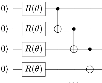
[image:28.612.212.378.92.228.2]

· · ·

Figure 1.1: An example quantum circuit diagram. These diagrams are read from left to right, where horizontal lines denote a particular qubit, boxes represent a quantum gate, and lines shows the control relationship for multi-qubit gates. Shown here is a series of one-qubit rotations

pa-rameterized by an angle theta, R(θ), followed by CNOT gates, where the solid dot represents the

control bit and the cross represents the target bit.

that can be used to express algorithms are quantum circuit diagrams, an example of

which is depicted in Fig. 1.1.

1.2.6 Electronic Hamiltonians

While the aim of almost all the methods in this work is to be generally applicable

to all quantum systems, electronic and chemical Hamiltonians are an application of

special interest. A non-relativistic system composed ofNn nuclei and Ne electrons

neglecting weak spin-spin interactions is defined by a Hamiltonian composed of the

the kinetic energy and Coulomb interactions of the charged particles. In atomic units

we write this Hamiltonian as

H = Ne X i=1 −∇2 ri 2 + Nn X i=1 −∇2 Ri

2Mi

+

Nn

X

i,j<i

ZiZj

|Ri−Rj|−

N_Xn,Ne

ij

Zi

|Ri−rj|

+

Ne

X

i,j<i

1 |ri−rj|

(1.39)

whereRi, Mi, Zi are nuclear positions, masses, and charges respectively, and the

(29)

be-tween the electrons and nuclei, this Hamiltonian can be well-approximated (in

non-dynamical problems) by assuming that the nuclei are fixed classical point charges.

This approximation is known as the Born-Oppenheimer approximation, and yields a

purely electronic Hamiltonian that depends only parametrically on the position of the

nuclei as

H=

Nn

X

i,j<i

ZiZj

|Ri−Rj|

+

Ne

X

i=1

−∇2

ri

2 −

N_Xn,Ne

ij

Zi

|Ri−rj|

+

Ne

X

i,j<i

1 |ri−rj|

. (1.40)

It is also known, both from experimental inference and later the spin-statistics

the-orem of quantum field theory, that electrons must be antisymmetric with respect to

exchange. One way of dealing with the antisymmetry is through explicit constraints

on wavefunctions, as in previous sections where we references antisymmetric

coef-ficient tensor constraints or antisymmetric components. Another way is to include

antisymmetry in the Hamiltonian through the use of second quantization. In second

quantization one makes use of the operator algebra of fermion creation and

annihila-tion operators,a†_i andaj, to account for antisymmetry. Defining the anti-commutator

{A, B_}:=AB+BA, these satisfy the fermion anti-commutation relations

n

a†_i, a†_jo= 0 (1.41)

{ai, aj}= 0 (1.42)

n a†_i, aj

o

=δij (1.43)

(30)

{|ϕii}i. The Hamiltonian in this basis, now including antisymmetry, may be written

H =X

ij

hija†_iaj +

1 2

X

ijkl

hijkla

†

ia

†

jakal (1.44)

where the coefficients of the operators are defined as integrals of the interaction terms

over this single particle basis. More explicitly,

hpq =

Z

dσ ϕ∗_p(σ) −∇

2 r 2 − X i Zi

|Ri−r| !

ϕq(σ) (1.45)

hpqrs =

Z

dσ1 dσ2

ϕ∗_p(σ1)ϕ∗q(σ2)ϕs(σ1)ϕr(σ2)

|r1−r2|

(1.46)

whereσi now contains the spatial and spin components of the electron,σi = (ri, si).

This form of the electronic Hamiltonian has been particularly useful in the

devel-opment of correlated electronic structure calculations. In this work, we will use it to

help formulate the electronic structure problem on quantum computers. In order to

do this, we first need to map this problem, which is in the language of

indistinguish-able fermions, to the language of qubits, or distinguishindistinguish-able two-level systems. There

are now at least 3 known isomorphisms that may be used to accomplish this task, the

Jordan-Wigner, Parity, and Bravyi-Kitaev mappings [35,112,209]. In this

disserta-tion, we primarily utilize the Jordan-Wigner transformation that is defined by

a†_p = (Y

m<pσ

z

m)σp+ (1.47)

ap = (

Y

m<pσ

z

m)σp− (1.48)

σ± ≡(σx±iσy)/2 (1.49)

(31)

operators_{σx_{, σ}y_{, σ}z_} _{in the distinguishable qubit basis. However, an important}

as-pect of this transformation that will be used later, is that despite this non-locality,

the number of terms in the Hamiltonian is conserved up to a constant factor. Thus if

there areO(M4_{) terms in the original fermionic Hamiltonian, where}_M _{is the number}

of single particle basis functions used to discretize the Hamiltonian, then there will be

O(M4_{) terms in distinguishable qubit representation of the Hamiltonian.}

1.3 Chapter outline and summaries

1.3.1 Chapters 2, 3, and 4

In the first chapters of this thesis, we will describe, and subsequently improve upon, a

new quantum algorithm for the study of quantum chemistry with minimal

experimen-tal requirements. This method is called the Variational Quantum Eigensolver [196],

and can be applied to general eigenvalue problems on a quantum computer, but our

specific application goals at the time were focused on quantum chemistry.

Almost all quantum algorithms to date have been developed agnostic to the

avail-able hardware. That is, the approach is write down the best possible algorithm with

regards to cost for attaining the result one desires, assuming that one day a quantum

device will be capable of running that algorithm. However, many of the algorithms

that perform optimally in the asymptotic limit of size require extraordinary resources

for systems of interest.

For this reason, we proceeded with a different, co-design approach to quantum

com-putation. We consider both the problem and the available architecture

simultane-ously, to achieve an optimal solution for the given hardware. This is done by

(32)

and components that can be trivially performed on a classical computer, so as not to

waste expensive quantum resources.

To describe how we formulate this approach, we return to the variational principle

of quantum mechanics. This principle states that for a Hermitian operatorH with

eigenvectors and eigenvalues|Ψii, Ei ordered by value, that any approximate

wave-function_|ΨTi (obeying necessary symmetries) satisfies

hΨT|H|ΨTi

hΨT|ΨTi ≥

E0 (1.50)

Thus if we can create some state_|ΨTibased on a set of parameters {θi}, we can

im-prove the quality of the approximation to the ground state by choosing parameters

that minimize the expectation value of the energy.

The preparation of complex quantum states based on some set of parameters is an

area where quantum computers excel. Indeed any parametrizable sequence of gates

or repeatable sequence of quantum operations can be considered as a valid trial state

preparation. We call this general idea, the “quantum hardware ansatz”, and it allows

one to use the available hardware to define the limits of the simulation. On a

theoret-ical side, we have investigated the preparation of parameterizable ansatz states that

we believe to be both high-quality and not efficiently prepared or sampled from on a

classical computer. We believe multi-reference unitary coupled cluster [225] to be a

strong candidate in this regard.

Once a state is prepared, one needs a way to evaluate the energy in order to

im-prove the parameterization. One potential solution is to use quantum phase

estima-tion, but this returns us to techniques which are, at the time of writing,

(33)

the expectation value of the electronic Hamiltonian as

hΨT|H|ΨTi ≡ hHi= X

ij

hijha†_iaji+

X

ijkl

hijklha

†

ia

†

jakali (1.51)

=X

iα

gi_αhσ_αii+X

ijαβ

g_αβij hσ_αiσ_βji+... (1.52)

where the first line shows that the energy is explicitly obtainable through the

two-electron reduced density matrix, weighted by the precomputed values of the two-electronic

integrals. The second line is obtained through any of the aforementioned

transfor-mations(e.g. Jordan-Wigner or Bravyi-Kitaev) from fermions to qubits and

demon-strates that the energy may be efficiently evaluated through a weighted sum of Pauli

measurements on the system. Here the Greek indices denote the type of Pauli

ma-trix (I, X, Y, Z) and the Roman index runs over the number of qubits. Recall that the

number of terms in sum on the second line scales the same as the number of terms in

the first with respect to the number of spin orbitals, and only a partial tomography of

the quantum system is ever required.

Based on the value of the energy, a new set of parameters for the state preparation

can be determined through some non-linear minimization scheme, such as

Nelder-Mead simplex method or simulated annealing [73,180]. Classical computers are well

optimized to perform tasks like adding together the measurements and deciding on

new parameters in a non-linear optimization, suggesting a hybrid approach.

The approach can be qualitatively outlined as

1. Prepare a quantum state on a quantum device based on an established protocol

that depends on a set of parameters_{θi}i.

(34)

weighted summation on a classical computer.

3. Use a classical computer to decide a new set of parameters_{θi}i that lowers the

energy, and repeat until convergence.

This procedure takes advantage of a quantum computer’s ability to prepare and

efficiently sample select elements from complex quantum states, while offloading

mun-dane tasks such as addition and multiplication of scalars to a classical computer. In

doing so, we conserve precious quantum resources for what they do best. We call

this technique the variational quantum eigensolver and this is the subject of

Chap-ter 2, which includes an experimental implementation on a photonic quantum chip.

Since its initial formulation, we have done some work in optimizations for ion traps

in Chapter 3. Finally, we imported technology from classical quantum chemistry in

Chapter 4, and showed how the use of the appropriate basis could offer dramatic

sav-ings, not only in this method, but all those currently being considered for quantum

chemistry on quantum computers.

1.3.2 Chapters 5 and 6

The potential of quantum computers to help accelerate our simulations and

under-standing of chemistry are great, however this eventual promise is not the only reason

to study quantum computation and quantum information in chemistry. The

knowl-edge gained in this field has now helped to bolster both our understanding and

method-ology in both general physics and chemistry. In these Chapters we introduce another

such knowledge transfer from quantum computation to classical simulation of

(35)

The gate model of quantum computation, built from qubits and sequences of

uni-tary gates is only one model of quantum computation currently under consideration.

Another model of interest is that of adiabatic quantum computation [68]. In this

model, one encodes the solution to a problem in the ground state of some

Hamilto-nianHp, and prepares the ground state to this problem Hamiltonian through a slow

adiabatic evolution from a simple starting Hamiltonian HD, whose ground state is

easy to prepare. By the adiabatic theorem, if the evolution of the Hamiltonian from

HD toHp is slow enough, one remains in the ground state and the solution to the

problem is found. This is often written as a simple linear schedule between the two

Hamiltonians parameterized by a real numbers_∈[0,1] as

H(s) = (1−s)HD +sHp. (1.53)

In order to unify this approach with the gate model, Kitaev, building off the work

of Feynman, developed the clock Hamiltonian, which encodes the result of a gate

model computation into the problem HamiltonianHp.

To perform this mapping, one attaches an ancilla quantum register that keeps

track of time, called the clock register. If one only has access to qubits then some

effort must be made to keep the clock states valid, however for classical computing

purposes, it suffices to use ad₋dimensional qudit, with orthonormal basis states

hi_|j_i = δij. Given an initial state|Ψ0i and an ordered sequence of quantum gates

(36)

these operations as its ground state is

Hc= X

t

1 2

I_{⊗ |}t_{i h}t_{| −}Ut⊗ |t+ 1i ht| −Ut†⊗ |ti ht+ 1|+I⊗ |t+ 1i ht+ 1|

+ (1_{− |}Ψ_{0i h}Ψ_0|)_{⊗ |}0_{i h}0_|. (1.54)

where the final projector is penalty term that breaks the degeneracy of the ground

state to the unique evolution desired. The properties of this Hamiltonian have been

studied extensively, and it is known that it is frustration-free and has a spectral gap

that decreases as 1/T2 _where_T _{is the total number of discrete time steps under}

con-sideration [33,34,49]. The ground state of this Hamiltonian is the history state,

|ΦHi, which contains the entire quantum trajectory as

|ΦHi=

1 √

T X

t

|Ψti |ti (1.55)

where_|Ψti is the state of the quantum system after the application of the first t−1

gates. The eigenvalue of this state is 0 by construction, though it may be adjusted

through a constant shift factor if desired.

In Chapter 5, we show that this can be derived from a more general discrete time

variational principle, and that recasting a dynamics problem as an eigenvalue problem

in this manner can have practical computational benefits on a classical computer. In

particular, we show that it makes parallel-in-time dynamics possible through use of

a proper preconditioner. Moreover the proposed algorithm demonstrates an

advan-tage over the current standard Parareal algorithm [14,143] for the quantum dynamics

problems studied.

(37)

corre-lated many-body systems, namely the Full Configuration Interaction Quantum Monte

Carlo (FCIQMC) [26,27, 29,128,213,220], technique can be applied to time

dy-namics problems with this connection. It suggests a close link between the fermion

sign problem experienced in the simulation of electronic ground states and the

dy-namical sign problem arising in the simulation of quantum dynamics. We introduced

a rotating basis methodology capable of mitigating the sign problem through

approxi-mate pre-computation and demonstrated the method’s capabilities in parallel

compu-tation of quantum circuits.

1.3.3 Chapter 7

The simulation of explicit wavefunctions has pushed forward by exploiting expert

knowledge of physics to identify structure and reduce the complexity of the

prob-lem to be solved. For example, the use of symmetry or knowledge that an

interac-tion is relatively weak with regards to another in perturbainterac-tion theory facilitates fast,

accurate approximations. Recently a technique has emerged in the field of signal

pro-cessing that attempts to exploit a different kind of structure, namely sparsity. These

techniques are generally referred to as compressed sensing methodologies [193,232].

A Hamiltonian governing many non-interacting particles may be written as the sum

of the non-interacting pieces

H =X

i

Hi (1.56)

(38)

given by a rank 1 quantum state

|Φ_i=_|φ1i |φ2i...|φNi (1.57)

whereHi|φii = Ei|φiiand as a result H|Φi = (P_iEi)|Φi. If one introduces some

weak coupling between the subsystems, we conjecture that one does not expect the

rank of the state to change dramatically and as such the state may be well described

by a CP-decomposition with rank r << D = MN_{. If this conjecture is true, the}

practical question is how to obtain this type of sparse representation without first

knowing the full state. Moreover, once the technique is developed, one would like to

examine what kind of systems exhibit such a decomposition.

In Chapter 7 we discuss the application of a method from the field of compressed

sensing, namely orthogonal matching pursuit combined with imaginary time evolution

to find exactly these types of compressed wavefunctions. The methodology we build

is general in the sense that it does not require that one use a specific type of ansatz

or apply it to a particular type of quantum system. As an example application we

consider the electronic structure of molecules, using an antisymmetric low rank

de-composition. We find solutions that are dramatically more compact than traditional

(39)

If you find that you’re spending almost all your time on

theory, start turning some attention to practical things;

it will improve your theories. If you find that you’re

spending almost all your time on practice, start turning

some attention to theoretical things; it will improve your

practice.

Donald Knuth

2

A variational eigenvalue solver on a photonic

quantum processor

∗

Abstract

Quantum computers promise to efficiently solve important problems that are intractable

on a conventional computer. For quantum systems, where the physical dimension

grows exponentially, finding the eigenvalues of certain operators is one such intractable

∗_{Alberto Peruzzo}_†_,_{Jarrod R McClean}_†_{, Peter Shadbolt, Man-Hong Yung, Xiao-Qi} Zhou, Peter J Love, Al´an Aspuru-Guzik, and Jeremy L O’Brien. A new variational eigenvalue solver on a photonic quantum processor. Nature Communications, 5(4213):1-7, 2014.

(40)

problem and remains a fundamental challenge. The quantum phase estimation

algo-rithm efficiently finds the eigenvalue of a given eigenvector but requires fully coherent

evolution. We present an alternative approach that greatly reduces the requirements

for coherent evolution and we combine this method with a new approach to state

preparation based on ans¨atze and classical optimization. We implement the algorithm

by combining a highly reconfigurable photonic quantum processor with a conventional

computer. We experimentally demonstrate the feasibility of this approach with an

ex-ample from quantum chemistry—calculating the ground state molecular energy for

He–H+_{. The proposed approach drastically reduces the coherence time requirements,}

enhancing the potential of quantum resources available today and in the near future.

2.1 Introduction

In chemistry, the properties of atoms and molecules can be determined by solving the

Schr¨odinger equation. However, because the dimension of the problem grows

expo-nentially with the size of the physical system under consideration, exact treatment

of these problems remains classically infeasible for compounds with more than 2–3

atoms [229]. Many approximate methods [102] have been developed to treat these

sys-tems, but efficient exact methods for large chemical problems remain out of reach for

classical computers. Beyond chemistry, the solution of large eigenvalue problems [206]

would have applications ranging from determining the results of internet search

en-gines [191] to designing new materials and drugs [86].

Recent developments in the field of quantum computation offer a way forward for

efficient solutions of many instances of large eigenvalue problems which are

(41)

eigen-values have previously relied on the quantum phase estimation (QPE) algorithm.

The QPE algorithm offers an exponential speedup over classical methods and

re-quires a number of quantum operationsO(p−1_{) to obtain an estimate with precision}

p [1,2,6,8,136,251]. In the standard formulation of QPE, one assumes the

eigenvec-tor |ψi of a Hermitian operatorHis given as input and the problem is to determine

the corresponding eigenvalue λ. The time the quantum computer must remain

coher-ent is determined by the necessity of O(p−1_{) successive applications of}_e−iHt_{, each of}

which can require on the order of millions or billions of quantum gates for practical

applications [111,251], as compared to the tens to hundreds of gates achievable in the

short term.

Here we introduce an alternative to QPE that significantly reduces the

require-ments for coherent evolution. We have developed a reconfigurable quantum processing

unit (QPU), which efficiently calculates the expectation value of a Hamiltonian (H),

providing an exponential speedup over exact diagonalization, the only known exact

solution to the problem on a traditional computer. The QPU has been experimentally

implemented using integrated photonics technology with a spontaneous parametric

downconversion single photon source and combined with an optimization algorithm

run on a classical processing unit (CPU), which variationally computes the

eigenval-ues and eigenvectors of H. By using a variational algorithm, this approach reduces

the requirement for coherent evolution of the quantum state, making more efficient

use of quantum resources, and may offer an alternative route to practical

(42)

QPU

Algorithm 1

Algorithm 2

CPU

quantum module 1

quantum state preparation

classical adder

classical feedback decision

quantum module 2 quantum module 3

quantum module n

[image:42.612.140.475.93.288.2]

Adjust the parameters for the next input state

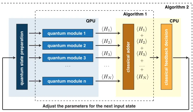
Figure 2.1: Architecture of the quantum-variational eigensolver. (Algorithm 1): Quantum states

that have been previously prepared, are fed into the quantum modules which compute _hHii, where

Hi is any given term in the sum defining H. The results are passed to the CPU which computes

hHi. (Algorithm 2): The classical minimization algorithm, run on the CPU, takes_hHi and

deter-mines the new state parameters, which are then fed back to the QPU.

2.2 Results

2.2.1 Algorithm 1: Quantum expectation estimation

This algorithm computes the expectation value of a given Hamiltonian_Hfor an input

state|ψi. Any Hamiltonian may be written as

H=X

iα

hi

ασαi +

X

ijαβ

hij_αβσi

ασ

j

β+... (2.1)

for realh where Roman indices identify the subsystem on which the operator acts,

and Greek indices identify the Pauli operator, e.g. α = x. Note that no

assump-tion about the dimension or structure of the hermitian Hamiltonian is needed for this

(43)

that

hHi=X

iα

hi_αhσ_αii+X

ijαβ

hij_αβhσi_ασ_βji+... (2.2)

We consider Hamiltonians that can be written as a number of terms which is

polyno-mial in the size of the system. This class of Hamiltonians encompasses a wide range

of physical systems, including the electronic structure Hamiltonian of quantum

chem-istry, the quantum Ising Model, the Heisenberg Model [147,153], matrices that are

well approximated as a sum of n-fold tensor products [188,189], and more

gener-ally any k₋sparse Hamiltonian without evident tensor product structure (see

Sup-plementary Information for details). Thus the evaluation of hHireduces to the sum

of a polynomial number of expectation values of simple Pauli operators for a

quan-tum state |ψi, multiplied by some real constants. A quantum device can efficiently

evaluate the expectation value of a tensor product of an arbitrary number of simple

Pauli operators [188]. Therefore, with ann-qubit state we can efficiently evaluate the

expectation value of this 2n_×₂n _Hamiltonian.

One might attempt this using a classical computer by separately optimizing all

re-duced states corresponding to the desired terms in the Hamiltonian, but this would

suffer from the N-representability problem, which is known to be intractable for both

classical and quantum computers (it is in the quantum complexity class QMA-Hard [145]).

The power of our approach derives from the fact that quantum hardware can store a

global quantum state with exponentially fewer resources than required by classical

hardware, and as a result the N-representability problem does not arise.

As the expectation value of a tensor product of an arbitrary number of Pauli

oper-ators can be measured in constant time and the spectrum of each of these operoper-ators is

(44)

coeffi-cienth, which is an arbitrary element from the set of constants _{hij..._αβ..._}, our approach

incurs a cost ofO(|h|2 _p−2_{) repetitions. Thus the total cost of computing the}

expecta-tion value of a state _|ψ_iis bounded byO(_|hmax|2 M p−2), where M is the number of

terms in the decomposition of the Hamiltonian andhmax is the coefficient with

maxi-mum norm in the decomposition of the Hamiltonian. The advantage of this approach

is that the coherence time to make a single measurement after preparing the state is

O(1). Conversely, the disadvantage of this approach with respect to QPE is the

scal-ing in the total number of operations as a function of the desired precision is

quadrat-ically worse (O(p−2_{) vs}_O₍_p−1_{)). Moreover, this scaling will also reflect the number of}

state preparation repetitions required, whereas in QPE, the number of state

prepara-tion steps is constant. In essence, we dramatically reduce the coherence time

require-ment while maintaining an exponential advantage over the classical case, by adding a

polynomial number of repetitions with respect to QPE.

2.2.2 Algorithm 2: Quantum variational eigensolver

The procedure outlined above replaces the long coherent evolution required by QPE

by many short coherent evolutions. In both QPE and Algorithm 1 we require a good

approximation to the ground state wavefunction to compute the ground state

eigen-value and we now consider this problem. Previous approaches have proposed to

pre-pare ground states by adiabatic evolution [6], or by the quantum Metropolis

algo-rithm [226,262]. Unfortunately both of these require long coherent evolution.

rithm 2 is a variational method to prepare the eigenstate and, by exploiting

Algo-rithm 1, requires short coherent evolution. AlgoAlgo-rithms 1 and 2 and their relationship

are shown in Figure 2.1 and detailed in the Supplementary Information.

(45)

D1

D2

D3

D4

CPU Optimization

algorithm

dc1 dc2

dc3

dc9 dc6

dc7

dc8

dc10

dc11 dc12 dc13 dc4 dc5

QPU

(a)

(b)

from SPDC source

from CPU

QPU to detectors

from SPDC source

from CPU

QPU to detectors

[image:45.612.133.474.93.344.2]

1 cm

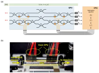
Figure 2.2: Experimental implementation of our scheme.(a) Quantum state preparation and

measurement of the expectation values_hψ|σi⊗σj|ψiare performed using a quantum photonic

chip. Photon pairs, generated using spontaneous parametric down-conversion are injected into the

waveguides encoding the _|00istate. The state_|ψiis prepared using thermal phase shiftersφ1−8

(orange rectangles) and one CNOT gate and measured using photon detectors. Coincidence count

rates from the detectors D1−4are passed to the CPU running the optimization algorithm. This

computes the set of parameters for the next state and writes them to the quantum device. (b) A photograph of the QPU.

operator_H can be restated as a variational problem on the Rayleigh-Ritz quotient [204,

205], such that the eigenvector_|ψ_i corresponding to the lowest eigenvalue is the_|ψ_i

that minimizes

hψ_{| H |}ψ_i

hψ|ψi . (2.3)

By varying the experimental parameters in the preparation of _|ψ_i and computing the

Rayleigh-Ritz quotient using Algorithm 1 as a subroutine in a classical minimization,

(46)

sim-ple prescription for the reconstruction of the eigenvector is stored in the final set of

experimental parameters that define|ψi.

0 1

0 20 40 60 80 100

−3 −2.5 −2 −1.5 −1 −0.5

Optimization step j

Energy (MJ mol

−1)

Energy levels Theoretical Experimental

Tangle

0 20 40 60 80 100

0

0.2 0.4 0.6 0.8

1

Optimization step j

State overlap

(a)

[image:46.612.186.422.148.422.2]

(b)

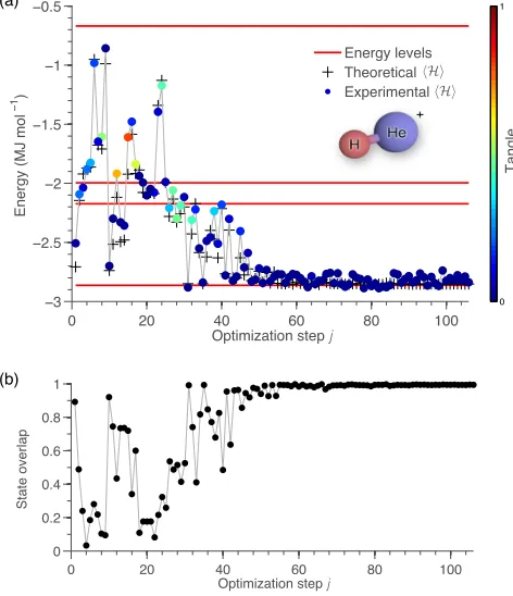
Figure 2.3: Finding the ground state of He-H+ for a specific molecular separationR = 90pm.

(a) Experimentally computed energy_hHi(colored dots) as a function of the optimization stepj.

The color represents the tangle (degree of entanglement) of the physical state, estimated directly

from the state parameters_{φji}. The red lines indicate the energy levels ofH(R). The

optimiza-tion algorithm clearly converges to the ground state of the molecule, which has small but non zero tangle. The crosses show the energy calculated at each experimental step, assuming an ideal

quan-tum device. (b) Overlap_{| h}ψj

|ψG

i | between the experimentally computed state_|ψj

iat each the

optimization stepj and the theoretical ground state of_H,_|ψG

i. Error bars are smaller that the

data points. Further details are provided in the Methods section and in the Supplementary Infor-mation.

If a quantum state is characterized by an exponentially large number of

parame-ters, it cannot be prepared with a polynomial number of operations. The set of

effi-ciently preparable states are therefore characterized by polynomially many

(47)

condi-tions, a classical search algorithm on the experimental parameters which define_|ψ_i,

needs only explore a polynomial number of dimensions—a requirement for the search

to be efficient.

One example of a quantum state parametrized by a polynomial number of

parame-ters for which there is no known efficient classical implementation is the unitary

cou-pled cluster ansatz [225]

|Ψ_i=eT−T†_|Φ_i_ref (2.4)

where |Φiref is some reference state, usually the Hartree Fock ground state, and T is

the cluster operator for anN electron system defined by

T =T1+T2+T3+...+TN (2.5)

with

T1 =

X

pr

tr_paˆ†_pˆar (2.6)

T2 =

X

pqrs

trs_pqaˆ†_pâ†_qârâs (2.7)

and higher order terms follow logically. It is clear that by construction the operator

(T −T†) is anti-hermitian, and exponentiation maps it to a unitary operatorU =

e(T−T†₎

. For any fixed excitation level k, the reduced cluster operator is written as

T(k)=

k X

i=1

Ti (2.8)

In general no efficient implementation of this ansatz has yet been developed for a

(48)

BCH series [225]. However this state may be prepared efficiently on a quantum

de-vice. The reduced anti-hermitian cluster operator (T(k)₋_T(k)†_{) is the sum of a}

poly-nomial number of terms, namely it contains a number of termsO(Nk₍_M₋_N₎k_{) where}

M is the number of single particle orbitals. By defining an effective Hermitian

Hamil-tonianH = i(T(k) ₋_T(k)†_{) and performing the Jordan-Wigner transformation to}

reach a Hamiltonian that acts on the space of qubits, ˜_H, we are left with a

Hamilto-nian which is a sum of polynomially many products of Pauli operators. The problem

then reduces to the quantum simulation of this effective Hamiltonian, ˜H, which can

be done in polynomial time using the procedure outlined by Ortiz et al. [188]. We

note that while this state preparation procedure utilizes tools from quantum

simu-lation, the total effective time of evolution is fixed by the expansion coefficients trs

pq.

This is in contrast to normal difficulties encountered in quantum phase estimation,

where simulations must be carried out for times that are exponential in the desired

final precision.

While there is currently no known efficient classical algorithm based on these ansatz

states, non-unitary coupled cluster ansatz is sometimes referred to as the “gold

stan-dard of quantum chemistry” as it is the stanstan-dard of accuracy to which other

meth-ods in quantum chemistry are often compared. The unitary version of this ansatz is

thought to yield superior results to even this “gold standard” [225].

2.2.3 Prototype demonstration

We have implemented the QPU using integrated quantum photonics technology [186].

Our device, shown schematically in Figure 2.2 is a reconfigurable waveguide chip that

can prepare and measure arbitrary two-bit pure states using several single qubit

(49)

of possible configurations with mean statistical fidelityF > 99% [210]. The state is

path-encoded using photon pairs generated via a spontaneous parametric

downcon-version process. State preparation and measurement in the Pauli basis is achieved by

setting 8 voltage driven phase shifters and counting photon detection events with

sili-con single photon detectors.

The ability to prepare an arbitrary two-qubit separable or entangled state enables

us to investigate 4_×4 Hamiltonians. For the experimental demonstration of our

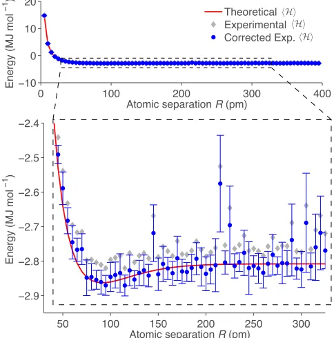
al-gorithm we choose a problem from quantum chemistry, namely determining the bond

dissociation curve of the molecule He-H+ _{in a minimal basis. The full configuration}

50 100 150 200 250 300

−2.9 −2.8 −2.7 −2.6 −2.5 −2.4

Atomic separation R (pm)

Energy (MJ mol

−1 )

0 100 200 300 400

−10

0 10 20

Atomic separation R (pm)

Energy (MJ mol

−1 ) _Theoretical

Experimental

[image:49.612.186.428.312.557.2]

Corrected Exp.

Figure 2.4: Bond dissociation curve of the He-H+ molecule. This curve is obtained by repeated

computation of the ground state energy (as shown in Figure 2.3) for several_H(R). The

Algorithms Bridging Quantum Computation and Chemistry

Algorithms Bridging Quantum

Computation and Chemistry

The Harvard community has made this

article openly available.

Please share

how

this access benefits you. Your story matters

Citation

McClean, Jarrod Ryan. 2015. Algorithms Bridging Quantum

Computation and Chemistry. Doctoral dissertation, Harvard

University, Graduate School of Arts & Sciences.

Citable link

http://nrs.harvard.edu/urn-3:HUL.InstRepos:17467376

Terms of Use

This article was downloaded from Harvard University’s DASH

repository, and is made available under the terms and conditions

applicable to Other Posted Material, as set forth at

http://

Algorithms Bridging Quantum

Computation and Chemistry

Algorithms Bridging Quantum Computation and

Chemistry

Contents

Citations to previously published work

Acknowledgments

1

Introduction

|

0

i

R

(

θ

)

•

|

0

i

R

(

θ

)

•

|

0

i

R

(

θ

)

•

|

0

i

R

(

θ

)

· · ·

2

A variational eigenvalue solver on a photonic

quantum processor

∗

_i

_•