laser-driven imploding target in cylindrical geometry. Physics of Plasmas. 012704. ISSN
1089-7674
https://doi.org/10.1063/1.3530596
[email protected] https://eprints.whiterose.ac.uk/ Reuse
Items deposited in White Rose Research Online are protected by copyright, with all rights reserved unless indicated otherwise. They may be downloaded and/or printed for private study, or other acts as permitted by national copyright laws. The publisher or other rights holders may allow further reproduction and re-use of the full text version. This is indicated by the licence information on the White Rose Research Online record for the item.
Takedown
If you consider content in White Rose Research Online to be in breach of UK law, please notify us by
9
Department of Physics, University of York, York, YO10 5DD, United Kingdom
10
University of California San Diego, La Jolla, California 92093, USA
11
LLNL, 7000 East Avenue, Livermore, California 94550, USA
共Received 19 October 2010; accepted 22 November 2010; published online 24 January 2011兲
An experiment was done at the Rutherford Appleton Laboratory 共Vulcan laser petawatt laser兲 to study fast electron propagation in cylindrically compressed targets, a subject of interest for fast ignition. This was performed in the framework of the experimental road map of HiPER 共the European high power laser energy research facility project兲. In the experiment, protons accelerated by a picosecond-laser pulse were used to radiograph a 220 m diameter cylinder 共20 m wall, filled with low density foam兲, imploded with⬃200 J of green laser light in four symmetrically incident beams of pulse length 1 ns. Point projection proton backlighting was used to get the compression history and the stagnation time. Results are also compared to those from hard x-ray radiography. Detailed comparison with two-dimensional numerical hydrosimulations has been done using a Monte Carlo code adapted to describe multiple scattering and plasma effects. Finally we develop a simple analytical model to estimate the performance of proton radiography for given implosion conditions. © 2011 American Institute of Physics.关doi:10.1063/1.3530596兴
I. INTRODUCTION
Many diagnostics1 have been used in inertial confine-ment fusion共ICF兲to follow the implosion dynamics, includ-ing proton radiography.2,3 Laser based proton source have also been used in this context, in particular for small-scale experiments performed in the framework of studies on the fast ignition approach to ICF.4Here the evolution of targets is imaged using the relatively low-energy共⬃10 MeV兲 pro-tons created by the interaction of high intensity 共1018– 1021 W/cm2兲 lasers with solid targets.
In this context, we performed an experiment at the Ru-therford Appleton Laboratory5 共RAL兲 in the framework of the HiPER roadmap6with the goal of studying the transport of fast electrons in cylindrically compressed matter.7–9 Pro-ton radiography was used together with hard x-ray radiogra-phy in the first phase of the experiment to record the implo-sion history of a cylindrical target. Experimental results were compared to simulations performed with the Monte Carlo codeMCNPX共Ref.10兲using the two-dimensional共2D兲 den-sity and temperature profiles of the imploding cylinder ob-tained with the hydrocodeCHIC.11–13Laser based protons are characterized by small source, high degree of collimation, and short duration. The multienergetic proton spectrum also allows probing the implosion at different times in a single shot, thanks to the difference in times-of-flight for protons at
different energies. This is a clear advantage over other diag-nostics共e.g., hard x-ray兲, which require several shots in order to follow the complete implosion history.
Another advantage of using proton radiography is a simple experimental setup keeping the imploding cylinder between the proton target and the proton detector on the same axis 共whereas x-ray radiography needs a complex ge-ometry, crystals, collimators, and detector alignment兲.
Proton radiography using laser-generated protons, and radiochromic films 共RCFs兲 as detectors, has already been used in an experiment at RAL共Refs. 4 and5兲 to probe the implosion of a spherical shell. Experimental results were analyzed and compared with Monte Carlo共MC兲simulations in Ref.4. However, the analysis done in Ref.4is based on the usual approach to proton imaging in which the proton energy loss during the target penetration is neglected assum-ing a direct correspondence between time-of-flight and stop-ping range of proton inside the detector. This approach has proven to be very successful in the detection of electric and magnetic fields in plasmas,14,15 but, as we will show in the following, it falls if applied to a the typical ICF. Starting from this point of view, in Ref.4the authors associated one RCF layer to a given probing time, and actually restricted most of their analysis to the image of the imploding shell obtained in the layer corresponding to the Bragg peak for 7
MeV, protons which they relied to a time of⬃2 ns after the beginning of laser irradiation 共⬃1 ns before stagnation兲. They observed significant differences between size of the shell predicted by the hydrocodes共85 mm兲 and the size re-corder on RCF images共120 mm兲. They justify this difference on the basis of the scattering of protons in the compressed core 共although, according to their estimates, they get 160 m兲and of the presence of electric and magnetic fields affecting proton trajectories.
In reality, as we will show in this paper, the problem mainly lies in the fact that, as protons are penetrating thick and dense targets, they do suffer severe multiple scattering 共MS兲effects and energy losses. This means that the共spatial兲 information carried on by the protons traveling in the central high density region of the target is lost and the image on the detector is mainly formed by the protons coming from the lower density regions. These effects have previously been considered in static proton radiography by Rothet al.,16 but acquire a new and deeper meaning in our dynamic situation, bringing to mixing of the images formed by protons with different energies. This implies that a more careful analysis of RCF images is needed, dropping the simple layer-to-time correspondence, and requiring detailed comparison with computer simulations. Whenever such analysis is done共see Sec. IV兲, we get a good agreement between experimental results and hydrosimulations.
The low density and hot temperature plasma corona play fundamental rules in formation of image on detector due to the relative low proton energy. Here indeed we show that at these conditions the stopping power共ST兲in plasma is higher than that in solid target. Finally, from the experimental point of view, in our work we could compare proton radiography results with those obtained by hard x-ray radiography, allow-ing to better understand the performance as well as the limi-tations of proton diagnostic, and to validate our interpretation of proton images.
II. EXPERIMENTAL SETUP
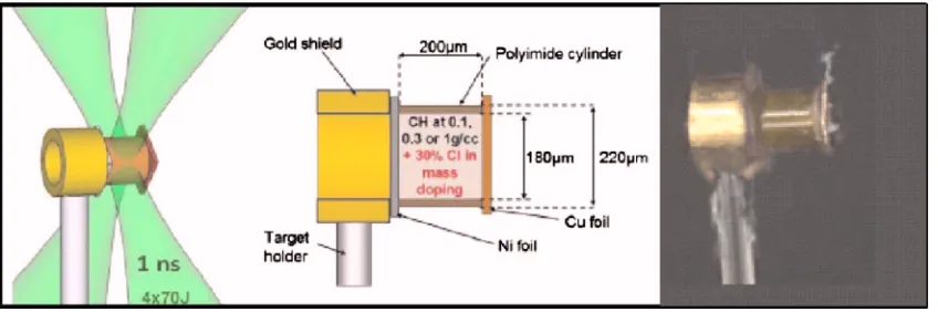
The experiment was carried out at the Vulcan facility using four long-pulse laser beams driving the implosion of cylindrical target. The beams共⬃4⫻50– 4⫻70 J in 1 ns at
= 0.53 m兲 were focused to 150 m full width at half
maximum共FWHM兲spots as shown in Fig. 1. A short pulse 共SP兲beam共100–150 J in 1 ps兲was focused as a backlighter source by an F= 3.5 off axis parabola with a focal spot 20 m FWHM at a peak irradiance of 1.5⫻1019 W/cm2to
produce protons for radiography. An intense beam 共10 ps, 160 J兲 is focused on a 25 m titanium foil providing the source for hard x-ray radiography ath⬇4.5 keV共details of such diagnostic will be presented in another paper兲.
The 200 m long polyimide cylindrical tube 共Fig. 1兲 with 220 m outer diameter and 20 m wall thickness was filled with foam 共acrylate兲 at density 0.1 g/cc, 1 g/cc, or empty. One side was closed with a Cu foil, the other side was closed by a Ni foil. The timing of the four long pulse共LP兲 beams was set so that they hit simultaneously the cylinder with the precision of ⫾50 ps due to the jitter. The delay between LP and SP was adjustable from 0 to 3.6 ns. The target was designed in order to generate plasmas with differ-ent values of density and temperature and thus differdiffer-ent plasma domains.
The experiment was split into two phases. The first phase objective was to determine the hydrodynamic charac-teristics of the compressed matter, i.e., its temperature and density at optimal compression while the second phase of the experiment was designed to measure the hot electron propa-gation through the compressed matter. In this paper we re-port about the first phase; for a complete rere-port of the second phase see Refs.7–9.
A. X-ray radiography setup
A SP laser beam 共10 ps, 160 J at = 1.064 m兲 was focused on a 25 m thick Ti foil placed at distance
d= 10 mm transversally of the target. The focal spot was 20 m diameter and the laser intensity on the foil was 5⫻1018 W/cm2. The generated x-rays were used to probe
the cylinder during the compression. The transmitted x-ray K␣ radiation 共Ti-Ka ⬃4.5 keV兲was selected via a spheri-cally bent quartz crystal 共quartz 203, 2d= 2.749 A,
Rc= 380 mm兲 at Bragg incidence 共Bragg⬃89: 5°兲 and
lo-cated at a distanceL1= 210 mm from the target on the
op-posite side of the Ti foil. The cylindrical target was imaged on to imaging plate, placed at L2⬃2 m away from the
[image:3.612.96.520.51.192.2]crystal共see Fig. 2兲. The total magnification of the imaging
system was MXR= 10.8 and the spatial resolution was ⌬x⬃20 m. The schematic is shown in Fig.2.
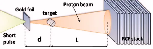
B. Proton radiography setup
Transverse point projection proton radiography4,9 was used to measure the target density during the compression. The proton backlighter source was realized using the SP laser beam from the Vulcan laser facility providing 100 J at 1.064 m in a 1 ps pulse. The laser beam was focused at normal incidence on a 20 m gold foil located at distance
d= 10 mm on the side of the cylindrical target. The obtained intensity on the gold foil was 3⫻1019 W/cm2 for a focal
spot of 20 m FWHM. The emitted proton beam from the Au foil’s rear side transversally probed the compressed cyl-inder. Protons had an approximately exponential spectrum with a cut-off energy of⬃10 MeV and they were collected by a stack of RCF composed of five layers of HD-810 and ten layers of MD55 positioned at a distance L⬃35 mm away from the target. The theoretical magnification of the system is MPR= 1 +L/d⬃4.5. A protective Al foil 共12 m
thick兲 was also positioned in front of the first RCF layer giving minimum detectable proton energy of⬃1 MeV the schematic is shown in Fig.3. The measured optical density on each RCF active layer is proportional to deposited energy.17
III. EXPERIMENTAL ANALYSIS
A. X-ray radiography results
Here we show the main results of x-ray radiography and refer for a more detailed analysis in Ref.8. X-rays are not affected by MS as protons are. The principal limitations of
the diagnostic lie in the imaging resolution power. The latter depends on the crystal quality, the x-ray source size, and the detector efficiency. The resolution power of the imaging sys-tem has been measured to be⌬x= 20 m by radiographing a metal grid whose dimensions 共step size and thickness兲 are known. On Fig. 4 a typical image of the cylinder is pre-sented, as obtained with the x-ray radiography. X-ray trans-mission profiles are extracted from radiographies by doing a lineout of the compressed part of the cylinder. Experimental diameters共FWHM兲are estimated by fitting the experimental transmission profiles with super-Gaussian of fourth order 共for early times, i.e., when the cylinder’s boundaries are still sharp兲 or Gaussian 共close to the stagnation time, i.e., when the blurring is more important兲functions.
B. Proton radiography results
The images recorded on RCFs were digitized with a Nikon 4.0 scanner with 4000 dots per inch resolution 共⬃6.5 m兲. In our experimental setup共see Fig.2兲the geo-metrical magnification was M= 4.5 allowing a spatial reso-lution of⬃1.5 m. We typically got seven impressed RCF layers per shot covering a full time span of 500 ps. Therefore we could not follow the whole target implosion in one shot, which implied the need to change the delay between SP and LP and reconstruct the full implosion with different shots 共typically three兲. The difference in Bragg peak energy be-tween two successive layers corresponded to a mean time-of-flight difference of⬃60 ps.
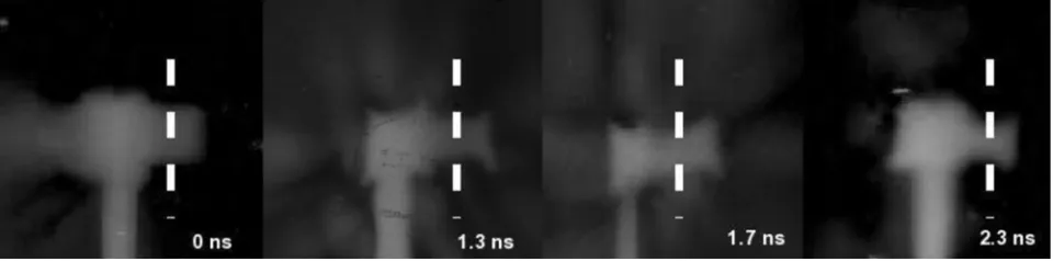
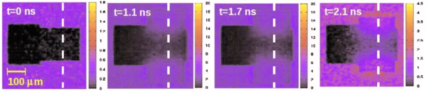
An example of experimental radiographs of the cylinder before compression 共reference shot兲 and of different stages of compressions is shown below in Fig.5.
[image:4.612.340.533.50.229.2]It is clear that compression along the longitudinal direc-tion 共cylinder axis兲 is not uniform. This is due to the finite size of the LP focal spots 共comparable to the cylinder length兲. However the focal spot was large enough to allow neglecting three-dimensional effects around its center. There-fore for each RCF image, we draw the optical density profile
FIG. 2. 共Color online兲Schematic of the x-ray radiography setup.
[image:4.612.53.299.59.210.2]FIG. 3. 共Color online兲Schematic of the proton radiography setup.
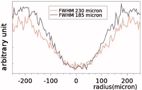
[image:4.612.54.301.662.741.2]at maximum compression共as shown later in Fig.8兲and mea-sured its FWHM. The optical density profile could be well interpolated by a super-Gaussian at early times共including the initially cold cylinder兲while approaching the stagnation time the fit becomes more Gaussian. This reflects the transition from a sharp cylinder boundary at early times to an extended plasma corona later. The measured widths were compared to the diameter of the compressed cylinder obtained by hydro-simulations, which assumed no variation of the intensity along the longitudinal direction. Let us also notice that com-pression was not uniform in the polar direction too, as a consequence of the small number of LP beams共only four兲. This implies a different target compression at 0°共direction of one of the incident LP beams兲and at 45°共direction exactly between two LP beams兲, an effect which was taken into ac-count by 2D simulations. Therefore the viewing angle of the proton diagnostic also needed to be considered when com-paring experimental results to hydro simulations usingCHIC
code.
The CHIC code includes bidimensional axisymmetrical hydrodynamics based on a cell-centered Lagrangian scheme, electron and ion conduction, thermal coupling, and detailed radiation transport. In our case, the ionization and opacity data are tabulated assuming a local thermodynamic equilib-rium, depending on the plasma parameters. The equations of state implemented in the code are based on a QEOS model13 or SESAME tables.14 Density 共Fig. 6兲, temperature 关Fig.7 共left兲兴, and ionization degree 关Fig. 7 共right兲兴 profiles at dif-ferent time during target compression, obtained by running
CHIC, are shown below.
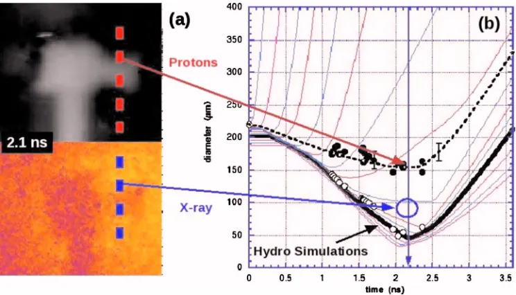
Figure8shows the time evolution of the cylinder diam-eter compared to the numerical prediction from the hydro-simulations in Figs.6 and7 for the case of a cylinder filled with 0.1 g/cc foam. It clearly shows the trend of compression of the target and it also reproduces the stagnation time given by simulations quite well共⬃2.1 ns兲. Note that the estima-tion of the stagnaestima-tion time was obtained starting from differ-ent hydroprofiles obtained byCHICcode relative to different laser energies in MC simulations共stagnation time is a strong function of driver energy兲and choosing the best fit with ex-perimental data 共the right parameters are those used in Fig. 6兲. It is clear however that the absolute value of the diameter of the compressed cylinder is not reproduced. In particular, the minimum observed diameter is ⬃140 m against ⬃50 m given by hydrosimulations 共see Fig. 6兲 for the
same stagnation time. Moreover the x-ray radiography re-sults confirm the hydrosimulations prediction giving a mini-mum observed diameter of⬃80 m. This fact implies that low energy protons are not able to probe the dense core as deeply as x-rays do.
IV. MC SIMULATION
In order to investigate the physical reason of the appar-ent contradiction among protons, x-ray results, and hydroex-pectation value showed in Fig.8, we have run MC simula-tions using the codeMCNPXdeveloped at LANL.10MCNPXis
[image:5.612.66.546.52.171.2]a general-purpose MC N-particle code that can be used for neutron, photon, electron, protons, and other particles trans-port. The MC code is able to reproduce the experimental setup in all its relevant parts: the proton source共energy spec-trum and spatial distribution of the proton source obtained from RCF analysis兲, the target and detector characteristic 共material composition, density profile, and geometry兲. ST of protons in the target is described by using Bethe’s theory18 while MS effects are described by Rossi’s theory.19
FIG. 5. Compression history obtained by experimental proton radiographs att1= 0 ns,t2= 1.3 ns,t3= 1.7 ns, andt4= 2.3 ns.
FIG. 6. 共Color online兲 Radial density profiles of cylindrical target before compression 共t= 0 ns兲 and during the compression phase
共t= 1.1, 1 , 7 , 2.1 ns兲. The simulations are performed withCHICcode using
[image:5.612.313.559.527.694.2]A. Plasma effects
Here we introduced some modifications in order to count for the differences between Bethe’s theory and the ac-tual ST in plasmas. Such “plasma effects,” connected to the variation of parameters共density, temperature, and ionization degree in Figs. 6 and 7兲 during target implosion, must be taken into account comparing MC simulations with experi-mental data and hydrodynamic simulations. Indeed in our experiment, there is a significant region共plasma corona兲in which the temperature becomes very high 关T⬃1 keV see Fig.7 共left兲兴which implies a large number of free electrons 共ionization degree兲with respect to the bound electrons and a correspondent enhancement of SP. Conventional MC codes
such asMCNPX, FLUKA, and SRIM do not take into account such effects because they were built to describe particle transport in cold matter共i.e., temperature and ionization ef-fects are not taken into account兲.
[image:6.612.73.542.51.222.2]A number of theoretical studies on ion beam interaction with plasmas are found in literature20,21and an experimental proof of the increase of the ion ST in ionized target material has been obtained in Ref. 22. A self-consistent theory of energy loss of ions in plasmas is given by means of the Vlasov–Poisson equations.21 Our analysis is developed within this framework and leads to the following formula for ST in partially ionized plasma共all the details are shown in the Appendix兲:
FIG. 7. Radial temperature共left兲and ionization degree共right兲profiles of cylindrical target during the compression phase共t= 1.1, 1 , 7 , 2.1 ns兲. The simulations are performed withCHICcode in the same conditions of Fig.6. Note that the ionization value 3.5 corresponds to the “mean” maximum ionization for the chemical composition of the compressed target.
[image:6.612.120.492.488.701.2]冉
dEdx
冊
= 1.23⫻10 −9 AEp
关qiLf+共Z−qi兲Lb兴, 共1兲
whereLf and Lb are, respectively, the free and bound elec-trons terms关Eqs.共A2兲and共A5兲兴. Equation共1兲represent the energy loss by protons with energy Ep共MeV兲 passing through partially ionized plasma with atomic and mass num-bersZ andA, density共g/cc兲, and ionization degreeqi. The
temperature effects are taken into account by the term Lf which is a function ofkbT共eV兲.
The general equation in Eq. 共1兲 leads to the Bethe ST formula18when qibecomes
冉
dEdx
冊
c= 1.23⫻10 −9 ZAEpln
冉
2149 EpI
¯
冊
共2兲and lead to the Bohr ST formula23 when qi becomes equal toZ
冉
dEdx
冊
p= 1.23⫻10 −9qiAEp
ln
冉
235.8冑
AEP3
qi
冊
. 共3兲
Comparison between Bethe and Bohr formula is shown in Fig.9 as a function of proton energy for the same material 共Mylar兲, temperatureT= 1 keV, and density= 0.1 g/cc.
This difference showed in Fig.9is principally due to the fact that free electrons are excited more easily than bound ones and it seems that it occurs predominantly for low den-sity regions 共e.g., ⬍1 g/cc兲. It is important to note that
Eqs.共1兲–共3兲are valid only in the classical free gas approxi-mation关Eq.共A10兲in the Appendix兴, i.e., for low density and high temperature as showed in Fig.18. One simple way to include plasma effects without changing the code inMCNPX
is to replace the “real” density profile 共Fig.6兲 h given by hydrosimulation with an “effective” profileecalculated by imposing the ST used byMCcode关Eq.共2兲兴to be the same as the one which takes place in plasma关Eq. 共3兲兴 in the region where the classical free gas approximations are satisfied,
冉
dE dx冊
c共e兲=
冉
dE
dx
冊
p共h兲. 共4兲
The effective density depends on the hydrodensity through a factorwhich depends on the density, temperature, and
ion-ization degree of the plasma and on proton energyEp,
e=h;=
qi
Z
冉
LfLb
+Z−qi
qi
冊
. 共5兲
Note that in the low density plasma corona region 共fully ionized plasmaqi=Z兲Eq.共5兲becomes ⬃Lf/Lb which im-plies that ifLf⬎Lbthen⬎1 ande⬎haccording to Fig.9 and with experimental results obtained in Ref. 23. On the other hand, in the solid target region共qi= 0兲Eq.共5兲becomes = 1 which impliese=h.
The above mentioned method affect also the estimation of the MS by the MC code introducing a magnification factor in the Rossi formula implemented in the code 共the Rossi formula was obtained in plasma configuration兲. We calcu-lated the error due to the magnification factor which is al-most everywhere less than 10% of the ST coefficient. In Fig. 10 are shown two different profiles obtained running MC simulation once with original density profile 共h兲 and the other with the modified one共e兲.
B. Proton energy spectrum
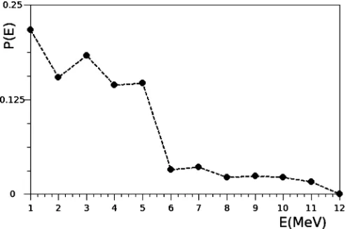
One of the most important ingredients for the MC simu-lations input file is the spatial and energy distribution of the initial proton beam. This essential information can be ob-tained by measuring the energy deposited in each RCF layer for a shot in which the cylindrical targets is removed 共i.e., protons traveling undisturbed兲 共Fig. 11兲. We had uncertain-ties deriving from shot-to-shot variations in energy and an-gular distribution of emitted protons.
[image:7.612.313.563.50.208.2]In particular, following Ref. 24, the energy deposited in thekth RCF layers 关Eq. 共6兲兴 is given by the convolution of the energy deposition curve B共zk,x,y,E兲 共characterized by the presence of the Bragg peak兲 and the proton energy dis-tributionP共E,x,y兲,
FIG. 9. 共Color online兲Proton stopping power as a function of energy for
cold共line below兲and warm matter共line above兲. corresponding to a Bragg peak forFIG. 10.共Color online兲MC simulation of proton energy deposition in layerEp= 3.2 MeV unperturbed protons共MC simulation without cylinder between proton source and detector兲, taken from the original hydro density profile关above black 共dark line兲兴 or using an effective density profile共plasma effects accounted for兲 关below red共lighter兲
[image:7.612.50.298.50.207.2]Sk共x,y兲=
冕
0
Emax
B⌬zk共x,y,Ep兲P共x,y,Ep兲dE;
共6兲
B⌬zk=
冕
⌬zk
B共z,x,y,Ep兲dz.
Assuming a discrete energy spectrum according to energy discretization emerging from RCF configuration 共the finite number of RCFs layers gives us information about finite value of energy only兲we can approximate the integral in Eq.
共6兲obtaining a matrix system which can be inverted in order to determine the spatial and energy spectrum of the initial proton beam.
In Fig.9is shown the spatial integrated initial spectrum functionP共Ei兲 as was obtained solving Eq.共6兲for different energies which are related to different RCF layers compared with the corresponding images for a shot without target “free shot.” The “almost”’-exponential form 共trapezoidal兲 of the spectral function agrees with typical spectral function form obtained in proton acceleration experiments共see for example Refs.24and25兲.
The spectral analysis of proton beam gives us fundamen-tal information:共i兲the integrated共over a RCFs surface兲 en-ergy spectrum共Fig.9兲and共ii兲the divergence as a function of energy共the angular divergence can be calculated starting from the diameter of the spatial profiles functions for each discrete energy and the proton source-detector distance兲. These results are implemented as initial condition for the MC simulations together with the density profiles obtained by
CHICcode modified following the scheme showed in the pre-vious section共plasma effects兲.
A quantitative analysis of the energy and spatial distri-butions of protons after they are passed through the cylinder has been done starting from RCF images obtained by shots with cylindrical target. The integrated energy spectrum of the proton beam after passing through the cylinder共see Fig. 9兲 shows a consistent reductions of number of particle in the low energy region 共Ep⬍4 MeV兲. This is due to the fact that proton with energy below that value of energy
over-comes a maximum areal density of the order of 13 mg/cc which is the typical mean value of the dense plasma core in our conditions.
C. Simulations results
Simulations of image formations were finally done as follows: 共i兲 We assume a time sampling of hydroprofiles 共density, temperature, and ionization degree共Figs.6 and7兲. 共ii兲 For each hydrotime, we run a MC simulation using the relative proton energy and protons number, calculating the energy deposition in each RCF layer. Each hydrotime corre-sponds to a different time-of-flight of incoming protons, i.e., to a different proton energy. 关The total number of particle 共normalized to 1兲used in all simulations must be equal to 1兴. However, here we consider the energy deposited by such protonsin allRCF layers and not only in the one correspond-ing to the Bragg peak of theemittedprotons, as it is usually done共of course, images will be formed only in RCF layers before that corresponding to the initial Bragg peak and in this one兲.共iii兲The full proton spectrum is covered running different simulations changing hydrotimes 共i.e., the hydro-profiles兲.
In this way, for each RCF layer we get a series of mo-noenergetic, fixed-time, 2D images. 共iv兲 Finally for each RCF layer, we sum all images at different times. In this way the resulting images on each layer will contain the contribu-tion of all the protons of the beam, which probed the target at different times共depending on their energy兲.
[image:8.612.51.298.51.215.2]The effects of image mixing is shown for instance in Fig. 12. Single energy images 共obtained by considering Bragg peak deposition only兲show a trend to increase target size as implosion proceeds, in disagreement with hydrosimulation results. Multienergy mixed images show instead the opposite trend. This is due to the fact that the convolution of the
FIG. 11. Spatial integrated initial spectrumP共E兲calculated inverting the matrix system obtained by the approximation of Eq.共6兲for the case of shot
without cylinder. FIG. 12.共Color online兲Comparison between FHWM of compressed cylin-der共shot 9兲by MC simulations obtained by using images on layers due to the respective Bragg peak energy共a兲or convolving all the proton energies contribution as a function of layers共time or energy兲for each layer共b兲. In the
[image:8.612.311.558.53.235.2]reduced energy 共therefore depositing their dose in another RCF layer兲, or finally, emerge with large scattering angles, so that they will be diffused over the entire layer surface. There-fore, the image formation will rather be done innegativeby protons traveling around the central part of the compressed cylinder.
Following the analysis procedure which we applied to experimental data, we have extracted FWHM by using Gaussian and super-Gaussian fits共Fig.14兲. We find, in agree-ment with experiagree-mental observations, a transition from super-Gaussian profiles at early times to Gaussian ones later in time.共Let us notice that in our synthetic images the com-pression is 2D, i.e., it is uniform in the direction of the inder axis. What we see at the edges of the compressed cyl-inder is simply due to modulation of MS effects兲. The full compression time is covered considering three different shots: shotn° 9 from 1.1 to 1.5 nsEmax⬃10 MeV, shotn° 5 from 1.5 to 1.9 nsEmax⬃10 MeV and shotn° 3 from 2.0 to 2.4 nsEmax⬃6 MeV.
V. PHYSICAL INTERPRETATION
The apparent difference between proton radiography ex-perimental and MC simulations results compared to the hy-drodynamical expectation value and x-ray radiography re-sults should be investigated more deeply in order to understand the physical meaning of this fact. In particular the relevant difference between proton 共charge particle兲 and x-ray共neutral particle兲 is given by the fact that protons in-teract with the Coulomb field of the nuclei that are within the probed matter. The number of those interaction is huge共i.e., MS兲and must be evaluated using statistical methods. In the following we investigate the MS phenomena and its influ-ence in PR resolution.
A. Multiple scattering effects
It is important to perform an analytical evaluation of MS because it is really the main responsible of the observed larger size of the proton images. This allows to evaluate the
right object size and also共as we will do in the last part of this paper兲to evaluate the necessary conditions for getting good proton radiographies.
We can estimate the effect of MS on thedetectedsize of the cylinder, by defining the blurring factor as
=L; =Es 2
冑
1
LR
冑
A关g/cm2兴E关MeV兴 ; A=
冕
−⬁ ⬁共x兲dx, 共7兲
whereAis a generalization of the areal density for cylindri-cal geometry共usuallyAis defined as the product of the den-sity times the longitudinal extension of the probed material兲,
Lis the distance between the cylinder and detector, is the mean angular deflection of a proton with energyEp travers-ing a material with density,Esis a constant= 15 MeV, and
[image:9.612.314.561.48.307.2]Lr is the radiation length,
FIG. 14.共Color online兲Comparison of experimental and simulation results. The point at 220 m shows the initial diameter of the cylinder; empty circles show simulated results obtained running hydro code CHIC, full ones the experimental points共dark in print兲and the simulated results running MCNPX MC code using hydro density profiles as input.
[image:9.612.94.521.648.741.2]Finally, the image formed on the layerkwill have a sizeDk given by the FWHM of the imageIk=兺Ii,kobtained by the convolution of all the imagesIk,i.
In principle, Eq. 共9兲 can be inverted deducing the real size of the cylinder for each layer. In order to estimate MS effect using the Rossi formula in Eq. 共7兲 we should calcu-lated the areal densityA关Eq. 共7兲兴. The areal density is usu-ally defined in planar target geometry as the product between the density of the material共which is assumed constant兲and the thickness of the target共along the direction perpendicular to the target surface兲. If the density profile along the longi-tudinal direction is not constant, this agrees with the so-called Gaussian approximation共the product of the peak den-sity with the FWHM兲. In this experiment 共and generally in all ICF experiments兲 the cylinder density profile cannot be represented by a Gaussian function共see Fig.6兲it is instead characterized by three regions: 共i兲 the plasma corona 共low density but large size兲,共ii兲the shocked region共high density short distance兲, and共iii兲the unperturbed target 共original tar-get density兲. Hence the proton traveling inside the tartar-get will see the value of the peak density only for short distance 共⬃20 m兲. In these conditions the Gaussian approximation leads to an overestimation of the blurring coefficient and the areal density must be calculated by detailed integration of the density profiles 关Eq. 共7兲兴. Moreover in this experiment the produced protons had a relatively low energy, the energy loss when they cross the target, and the MS effects are therefore quite large. In particular the protons passing through the dense core of the imploded target are scattered more than the protons passing through the external plasma corona so the images on layers are mainly formed innegativebyexternal
protons. In this case the areal density in Rossi’s formula must be calculated by integrating the density profile only in the plasma corona region共i.e., considering external protons only兲.
Figure 15 shows estimations of the cylinder size 共FWHM兲 for shot n° 9 using Rossi’s formula to calculate blurring coefficient and assuming different definition of the areal densityA. The estimation based on the Gaussian ap-proximation is far from simulation predictions while the es-timations based on numerical integration of the hydrodensity profile are more precise. It is important to note that, as we have mentioned before, for low energy共first layers兲A must be calculated only in plasma corona region.
The paper reported in Ref.4modeled the propagation of protons through the target using an algorithm based on the
SRIM code,10 which is in principle quite similar to MCPNX. However, the authors did not take into account the plasma effects and, as we already said, they only analyzed a single experimental image at fixed time neglecting the whole time evolution of the imploding target and the contributions from protons of different energies, i.e., they neglectedimage mix-ing. In this way they oversimplified the physical interpreta-tion of the experimental results. Furthermore they estimated MS effects in a wrong way, by calculating the blurring coef-ficient 关Eq. 共7兲兴 using density of the order of that of the compressed core关Fig.15共b兲兴, instead of the low density re-gion关Fig.15共c兲or Fig.15共d兲兴, which is typical of the plasma corona. The resulting blurring coefficient increases and the resulting size prediction isI⬃160 m, which is far from the experimental results I⬃120 m. Finally the authors were unable to justify the large target size observed in proton ra-diography images, and in order to explain the difference they claimed for additionalexoticeffects due to electric fields in the target. We have show in this paper that there is no need for such additional effect and that, if properly taken into account, the hydrodynamics alone can completely justify the observed images.
B. Proton radiography oesolution
In this paper we have shown that the mechanism of PR in warm dense matter 共ICF experiment兲 is quite different from that in cold matter due to the presence of a large num-ber of collisions. Many MC simulations were made4 but were never introduced any criterion for measuring the reso-lution of proton radiography in ICF.
[image:10.612.315.559.58.232.2]Here we want to define a criterion to estimate the reso-lution degree of the system starting from the parameters and the experimental setup. To do this let us consider the experi-mental setup shown in Fig.16共a兲in which a pointlike proton
FIG. 15.共Color online兲Estimation of cylinder size as a function of different layers共monoenergetic images for shotn° 9兲using Rossi’s formula关Eq.共7兲兴
and assuming different definition of the areal density:共a兲Gaussian approxi-mationA=L,共b兲numerical integration of density profile for protons trav-eling into the center of the compressed cylinderA关−rc,rc兴 共wherercis the core radius兲, 共c兲 numerical integration of density profile over all space
source irradiates a finite size object projecting its image on the detector. In principle, if the MS is negligible, the object will appear transparent共i.e., = 0兲 and the projected image size will appear enlarged by a factorM 关Eq.共9兲兴which cor-responds to the geometrical magnification.
More specifically, defining a generic distance between two points in the object␦x, the projected size on the detector becomes⌬x=M ␦x. Nevertheless the effect of the Coulomb MS is never negligible and the protons passing through the object are deflect by a mean angleqgiving a mean displace-ment=Lwhich can be estimate using the Rossi’s formula in Eq.共7兲.
Therefore the projected image on the detector will ap-pear enlarged by a factorwith respect to that would appear if there were no scattering ⌬x, i.e., by a factor M with respect to the initial distance␦x关we start from Eq.共9兲using
⌬xinstead of f兴,
=
冑
1 +冉
¯
␦x
冊
2; ¯=/M. 共10兲
Starting from the above considerations, we can infer that the blurring coefficient must remain less or of the same order than resolution that we would like to obtain dx in order to avoid the crossover between different single proton trajec-tory and the consequent loss of the initial spatial target in-formation’s carry on by protons.
The above-mentioned condition can be written in terms of blurring coefficient共i.e.,/M is the resolution of our sys-tem in analogy with Rayleigh’s criterion in optics兲
0ⱕ¯ⱕ␦x 共11兲
or in terms of thea-dimensional parameterm
1ⱕⱕ
冑
2. 共12兲We refer to the above condition 关Eqs. 共11兲and共12兲兴 as the “strong condition.” If the strong condition is satisfied we can use proton radiography in conventional way and the gray
scale obtained by the RCF analysis will be proportional to the density gradient of the probed target.
A simple estimation of the parameter can be done starting from the protons passing through the dense core in our case: the size of the core is⬃60 mm then we look for a resolution ␦x⬃20 m; the blurring coefficient /M can be estimated assuming the maximum energy for protons 共10 MeV兲, which are passing through an area density A
⬃0.05 g/cm2and a magnification factorM= 4.5. The result is⬃7 which is larger than the maximum permitted value in Eq.共12兲confirming that for low energy protons the strong condition cannot be applied because of they are not able to probe the dense core. On the other hand, assuming the plasma corona areal density A⬃0.002 g/cm2 at the same
conditions we obtain ⬃2 which is a more reasonable value.
In Fig. 17 is shown the mean scattering angle versus areal density for different proton energy. Typical value for our experiment is shown. The maximum resolution obtained in the region of the plasma corona at the RAL-08 experiment is about 20m due to the low energy of the probed protons 共⬍10 MeV兲, while if we would like to probe a typical core density target in omega27 we need to use a very high energy proton beam共⬃250 MeV兲.
The grey region corresponds to the ST limit obtained by fitting simulations based on the ions ST formula in Eq.共1兲. In particular we calculated the minimum energy required for a proton to overcome certain areal density of carbon 共Z= 6 A = 12兲 Em关MeV兴 ⬇30
冑
A关g/cm2兴. Inserting the minimum energy into the Rossi formula for the mean scat-tering angle 关Eq. 共7兲兴 we obtain the maximum scattering angle for proton to overcome certain areal densitym⬇
冑
A关g/cm2兴/Em关MeV兴 ⬇1.9°共i.e., protons with scatter-ing angles lower than the maximum will overcome the areal density兲.The above considerations suggest that proton
[image:11.612.93.515.52.245.2]phy technique can be used for ICF only under specific con-ditions which depend also on the geometrical features of the experiment.
As example let us assume very sharp target density pro-files; as just explained before, protons which pass through the dense core are stopped or diffuse while those which pass through the corona are deviated by a mean scattering angle which could be acceptable. Thanks to the sharp profiles, the differences in areal density between the external and the in-ternal protons become be very huge giving a high contrast and then an acceptable resolution.
Here we developed a criterion to estimate the resolution of the system in the above mentioned condition as a function of the sharpness of the target profile and we refer to this criterion as “weak condition.”
Let start assuming a 2D super-Gaussian density profile 共whereg is related to slope of the distribution兲
Ax,y共␥兲=pexp
冋
− ln 2冉
x␥+y␥
w␥
冊
册
共13兲共where we have definedw= FWHM/2兲. Protons arriving by
thex-direction will probe certain density profilesAy共g兲 as a function of theiry position
Ay共␥兲=
冕
RAx,y共␥兲dx=Ax共␥兲exp
冋
− ln 2冉
x
w
冊
␥
册
;共14兲
Ax共␥兲=p
冕
Rexp
冋
− ln 2冉
xw
冊
␥
册
dx. The resulting Blurring coefficient will bey共␥兲=
⌫c
冑
Ay共␥兲Ep
=⌫c
冑
Ax共␥兲Ep
exp
冋
−ln 2 2冉
x
w
冊
␥
册
;共15兲
the FWHM兲must be larger than the two FWHMs of the target density profiles,
共I兲共w+2w兲共␥兲⬍2w; 共II兲共w−2w兲共␥兲⬎4w.
The above conditions can be rewritten as follows:
共I兲2共1/2兲关1 + 2兴␥−⌫c
冑
Axp 2wEp⬎0;
共II兲ln 2
2 关共1 + 2兲
␥−共1 − 2兲␥兴+ ln
冉
2
冊
⬎0.The共i兲condition depends on the experimental parameters共,
Ep,w,⌫兲 and on the geometry of the target density profiles 共␥,兲it gives us the resolution of proton radiography for all the protons passing outside of the core which is defined by the FWHM. The共ii兲 condition depends on the geometry of the target density profiles 共␥,兲 and it guarantees that the protons passing through the core do not participate to form the image on layer.
Of course in the weak condition regime we accept to loss all the information about the internal core of the target and we look at its size only.
From experimental point of view the super-Gaussian de-greeg is not convenient in anyway we can use the relation between the Gaussian degreeg and the slope of the density profiles calculated inw关A
⬘
共w兲兴A
⬘
共w兲=ln 2 2冉
p
w
冊
␥. 共16兲Let us check the weak condition for the two interesting cases: RAL-08 共Refs. 10 and 11兲 and omega typical experiments.25 The 共ii兲 condition is independent on the experimental parameters and it leads to the conditions:
␦x⬎20 m for ␥= 2 and ␦x⬎10 m for ␥= 4. The 共i兲_ condition gives ␦x⬎85 m for ␥= 2, ␦x⬎30 m for ␥= 4, and␦x⬎15 m for␥= 6 for the RAL-08 experi-ment共⬃5 g/cc,E⬃10 MeV, w⬃60 m兲, and gives␦x ⬎90 m for␥= 2, ␦x⬎30 m for␥= 4, and ␦x⬎18 m for ␥= 6 for a typical omega target 共A⬃0.2, E⬃15 MeV,
w⬃60 m兲.
VI. CONCLUSIONS
PR has been used to diagnose the implosion of cylindri-cal targets, but a detailed analysis is required in order to allow comparison with hydrosimulations. The simple
RCF-FIG. 17.共Color online兲Mean scattering angleqvs areal density for differ-ent proton energies. xa A⬃0.004 g/cm2 proton trajectory calculated
through plasma corona andxbA⬃0.05 g/cm2trajectory through core for
the present experiment, andxcA⬃0.2 g/cm2trajectory共theory兲for a
typi-cal omega target共Ref.27兲. If we assumed=L= 1 cm共M= 2兲we get the corresponding spatial resolution limits:⬃20 m,⬃10 m, or ⬃1 m
共horizontal dashed lines兲. The grey region corresponds to the ST limit
[image:12.612.52.299.51.203.2]history and stagnation time are reproduced correctly, low-energy protons are not able to probe the dense core directly. MS is reduced for high-energy protons and, with respect to this problem, we have deduced two different criteria to pre-dict the minimum energy needed in order to reach a good resolution in ICF experiments.
ACKNOWLEDGMENTS
The authors acknowledge the support of the HiPER project and Preparatory Phase Funding Agencies 共EC, MSMT, and STFC兲in undertaking this work.
APPENDIX: PROTON ST
For our intent we prefer to write all the formulas in unit of MeV for proton beam energyEp, g/cc for density of the probed material, and eV for the temperature kbT of the plasma. We start writing the classical nonrelativistic Bethe SP formula for cold matter,17
冉
dE dx冊
c= 1.23⫻1023 Z
AEp
Lb, 共A1兲
where
ln
冉
2149EpI
¯
冊
; I¯= 8Z
冉
1 +1.8冑
Z冊
. 共A2兲Equation共A1兲represents the energy loss by proton with en-ergy Ep passing through a material with atomic and mass numbersZ andA and solid densityc=共A/Z兲共nb/Na兲where
nbis the bound electrons density, andNathe Avogadro num-ber and is the mean ionization potential. When the proton beam passes through a plasma instead of cold matter, Eq.
共A1兲is not able to describe all the physical phenomena oc-curring during the interaction as for example the temperature effects. The right SP formula can be obtained starting from a self-contained representation of the theory of energy loss of ions penetrating classical plasma given by nonrelativistic Vlasov–Poisson equations,19
冋
t+vជ·rជ+ e
m共rជ兲·vជ
册
f共r៝,v៝,t兲= 0;
共A3兲
ⵜ2
= − 4Ze␦共r៝−v៝t兲+ 4e
冕
f共r៝,v៝,t兲d3v− 4n0e which leads to the following solution:H共x兲= x
3
3
冑
2ln共x兲exp共−x2/2兲
+ x
4
x4+ 12, 共A7兲
x= 33
冑
EpKbT
; 共A8兲; d= 7.6⫻10−12
冑
AKbTEp
qip ,
共A8兲
k=Min关7.46⫻1011共E
p+ 1.8⫻10−3KbT兲,2.4
⫻1011
冑
Ep兴. 共A9兲Here d is the Debye length in unit of m, k in m−1 is the inverse of the impact parameter, andp=共A/qi兲共nf/Na兲is the plasma density withnf defined as the free electron density. The above equations can be derived assuming two conditions which must be always satisfied:19 共c1兲 Free gas Maxwell– Boltzmann statistic approximation and共c2兲collisionless ap-proximation.
With our notation the above conditions can be written as
KbT关eV兴⬎66.7
冉
qi
A
冊
2/32/3关g/cc兴 ⬇K
bT⬎422/3,
共A10兲
KbT关eV兴⬎58.8
冉
qiA
冊
1/31/3关g/cc兴 ⬇KbT⬎46.71/3.
共A11兲
Assuming a completely ionized 共qi= 6兲 carbon target 共A= 12兲we obtain:
Figure18shows the region of temperature-density plane 关completely ionized共qi= 6兲 carbon target 共A= 12兲兴in which conditions c1 and c2 are satisfied. The filled circles represent the three different state of the target in RAL-08 experiment. Note that SP formula in Eq. 共A5兲 is able to describe the energy loss by protons in the plasma corona region only and partially in the plasma core region 共high density and tem-perature兲. The cold region can be described also by Eq.共A5兲
in the limit of nonionized plasma共qi= 0, i.e., solid state兲in which it becomes equal to Eq. 共A4兲. For ICF physics, the temperature of the proton beam which probed the target 共⬃10 MeV兲 is always greater than the temperature of the probed plasma 共⬃1 KeV兲, then the free term in Eq. 共A5兲
becomes
共A5bis兲Lf⬇ln
冉
60冑
AEp2
qip
冊
共A12兲
共A6bis兲
冉
dE
dx
冊
p= 1.23⫻10 −9qiAEp
冋
ln
冉
60冑
AEp2
qip
冊
+共Z−qi兲
qi
ln
冉
2149EpI
¯
冊
册
. 共A13兲1
Advanced Diagnostics for Magnetic and Inertial Fusion, edited by E. Stott, A. Wootton, G. Gorini, and D. Batani共Plenum, New York, 2002兲.
2
J. R. Rygg, F. H. Séguin, C. K. Li, J. A. Frenje, M. J.-E. Manuel, R. D. Petrasso, R. Betti, J. A. Delettrez, O. V. Gotchev, J. P. Knauer, D. D. Meyerhofer, F. J. Marshall, C. Stoeckl, and W. Theobald,Science 319,
1223共2008兲.
3
A. J. Mackinnon, P. K. Patel, M. Borghesi, R. C. Clarke, R. R. Freeman, H. Habara, S. P. Hatchett, D. Hey, D. G. Hicks, S. Kar, M. H. Key, J. A. King, K. Lancaster, D. Neely, A. Nikkro, P. A. Norreys, M. M. Notley, T. W. Phillips, L. Romagnani, R. A. Snavely, R. B. Stephens, and R. P. J. Town,Phys. Rev. Lett. 97, 045001共2006兲.
4
M. Borghesi, A. Schiavi, D. H. Campbell, M. G. Haines, O. Willi, A. J. MacKinnon, L. A. Gizzi, M. Galimberti, R. J. Clarke, and H. Ruhl,Plasma Phys. Controlled Fusion 43, A267共2001兲.
5
C. N. Danson, L. J. Barzanti, Z. Chang, A. E. Damerell, C. B. Edwards, S. Hancock, M. H. R. Hutchinson, M. H. Key, S. Luan, R. R. Mahadeo, I. P. Mercer, P. Norreys, D. A. Pepler, D. A. Rodkiss, I. N. Ross, M. A. Smith, R. A. Smith, P. Taday, W. T. Toner, K. W. M. Wigmore, T. B. Winstone, R. W. W. Wyatt, and F. Zhou,Opt. Commun. 103, 392共1993兲.
6
M. Dunne, F. Amiranoff, S. Atzeni, J. Badziak, D. Batani, S. Borneis, J. L. Collier, C. N. Danson, J. C. Gauthier, J. J. Honrubia, M. H. R. Hutchinson, S. Jacquemot, M. Koenig, K. Krushelnick, T. Mendonca, P. V. Nickles, P. A. Norreys, S. J. Rose, J. Wolowsk, N. Woolsey, M. Zepfet al.“HiPER, technical background and conceptual design,” Rutherford Appleton Labo-ratory Report No. RAL-TR-2007–008, 2007.
Perez, F. Dorchies, J. J. Santos, C. Fourment, S. Hulin, P. Nicolai, B. Vauzour, K. Lancaster, M. Galimberti, R. Heathcote, M. Tolley, Ch. Spindloel, P. Koester, L. Labate, L. Gizzi, C. Benedetti, A. Sgattoni, M. Richetta, J. Pasley, F. Beg, S. Chawla, D. Higginson, A. MacKinnon, A. McPhee, D.-H. Kwon, and Y. Rhee,J. Korean Phys. Soc. 57, 305共2010兲. 10
M. L. Fensin, J. S. Hendricks, and S. Anghaie, J. Nucl. Sci. Technol.170,
68共2010兲; F. Ziegler, J. P. Biersack, and M. D. Ziegler,The Stopping Power of Ions in Matter共Lulu Press, Morrisville, North Carolina, 2009兲.
11
P. H. Maire, J. Breil, R. Abgral, and J. Ovadia,SIAM J. Sci. Comput.
共USA兲 29, 1781共2007兲. 12
A. J. Kemp and J. Meyer-ter-Vehn,Nucl. Instrum. Methods Phys. Res. A
415, 674共1998兲 13
T4 Group, “SESAME Report on the Los Alamos Equation of State Li-brary,” Los Alamos National Laboratory, Los Alamos Report No. LALP-83-4.
14
M. Borghesi, A. J. Mackinnon, D. H. Campbell, D. G. Hicks, S. Kar, P. K. Patel, D. Price, L. Romagnani, A. Schiavi, and O. Willi,Phys. Rev. Lett.
92, 055003共2004兲. 15
D. Batani, S. D. Baton, M. Manclossi, D. Piazza, M. Koenig, A. Benuzzi-Mounaix, H. Popescu, C. Rousseaux, M. Borghesi, C. Cecchetti, and A. Schiavi,Phys. Plasmas16, 033104共2009兲.
16
M. Roth, A. Blazevic, M. Geissel, T. Schlegel, T. E. Cowan, M. Allen, J.-C. Gauthier, P. Audebert, J. Fuchs, J. Meyer-ter-Vehn, M. Hegelich, S. Karsch, and A. Pukhov,Phys. Rev. ST Accel. Beams 5, 061301共2002兲. 17
Seehttp://www.gafchromic.com/for GAFCHROMIC HD-810 radiochro-mic dosimetry film and D-200 preformatted dosimeters for high-energy photons configurations.
18
H. Bethe, Ann. Phys.共N.Y.兲 5, 325共1930兲. 19
B. Rossi and K. Greisen,Rev. Mod. Phys. 13, 240共1941兲. 20
T. A. Mehlhorn,J. Appl. Phys. 52, 6522共1981兲. 21
T. Peter and J. Meyer-ter-Vehn,Phys. Rev. A 43, 1998共1991兲; 43, 2015
共1991兲.
22
F. C. Young, D. Mosher, S. J. Stephanakis, S.A. Goldtein, and T. A. Mehlhorn.,Phys. Rev. Lett. 49, 549共1982兲.
23
N. Bohr, Philos. Mag. 30, 581共1915兲. 24
E. Breschi,Nucl. Instrum. Methods Phys. Res. A522, 190共2004兲. 25
K. Zeil, S. D. Kraft, S. Bock, M. Bussmann, T. E. Cowan, T. Kluge, J. Metzkes, T. Richter, R. Sauerbrey, and U. Schramm,New J. Phys. 12,
045015共2010兲.
26
See http://pdg.lbl.gov/2008/AtomicNuclearProperties for PDG particle data group.
27
[image:14.612.51.298.54.220.2]University of Rochester-Laboratory for Laser Energetics Report No. DOGNA28503-923, January 2010.
FIG. 18.共Color online兲Temperature共eV兲vs density共g/cc兲plane. The filled circle regions represented by the graph represent the three different states of matter occurring in RAL-09 experiment. The region above the blue共darker兲
line共T⬎42p兲is that in which the conditions in Eq.共A11兲is satisfied while
the region above the red共lighter兲 line 共T⬎46.7p兲 is that in which the