Agent-Based Models for Causal Inference
The Harvard community has made this
article openly available.
Please share
how
this access benefits you. Your story matters
Citation
Murray, Eleanor Jane. 2016. Agent-Based Models for Causal
Inference. Doctoral dissertation, Harvard T.H. Chan School of Public
Health.
Citable link
http://nrs.harvard.edu/urn-3:HUL.InstRepos:27201721
Terms of Use
This article was downloaded from Harvard University’s DASH
repository, and is made available under the terms and conditions
applicable to Other Posted Material, as set forth at
http://
AGENT-BASED MODELS FOR CAUSAL INFERENCE
ELEANOR J. MURRAY
A Dissertation Submitted to the Faculty of
The Harvard T.H. Chan School of Public Health
in Partial Fulfillment of the Requirements
for the Degree of Doctor of Science
in the Department of Epidemiology
Harvard University
Boston, Massachusetts.
Dissertation Advisor: Dr. Miguel A. Hernán Eleanor J. Murray
ii
Agent-based Models for Causal Inference
Abstract
Sound clinical decision making requires evidence-based estimates of the impact of different
treatment strategies. In the absence of randomized trials, two potential approaches are agent-based
models (ABMs) and the parametric g-formula. Although these methods are mathematically similar, they
have generally been considered in isolation. In this dissertation, we bridge the gap between ABMs and
the parametric g-formula, in order to improve the use of ABMs for causal inference.
In Chapter 1, we describe bias that can occur when ABM inputs or estimates are extrapolated to
new populations, and demonstrate the impact of this bias by comparison with the parametric g-formula.
We describe the assumptions that are required for extrapolation of an ABM and show that violations of
these assumptions produce biased estimates of the risk and causal effect.
In Chapter 2, we describe an approach to provide calibration targets for ABMs, and to identify
the set of parameters of the ABM that interfere with transportability of the model results to a particular
population. We illustrate this approach by comparing the estimates from an existing ABM, the
Cost-Effectiveness of Preventing AIDS Complications (CEPAC) model, to estimates from the parametric
g-formula applied to a prospective clinical data of HIV-positive individuals under different treatment
initiation strategies.
In Chapter 3, we focus on the core problem of causal inference from ABMs: how to define and
estimate the parameters described in Chapter 2 in light of the bias described in Chapter 1. To illustrate
this problem, we consider CEPAC input parameters for opportunistic diseases. We formally define the
effect of interest, describe the conditions under which this effect is or is not identifiable, and describe
the assumptions required for transportability of this effect. Finally, we show that the estimation of these
iii
Table of Contents
LIST OF FIGURES WITH CAPTIONS ... V
LIST OF TABLES WITH CAPTIONS ... X
ACKNOWLEDGEMENTS ... XII
INTRODUCTION ... 1
CHAPTER 1 A COMPARISON OF AGENT-BASED MODELS AND THE PARAMETRIC G-FORMULA FOR CAUSAL INFERENCE ... 3
ABSTRACT ... 4
INTRODUCTION ... 5
A SIMPLIFIED DECISION ANALYSIS EXAMPLE ... 6
TREATMENT-CONFOUNDER FEEDBACK ... 9
BIAS EVEN IF THE ABM IS BASED ON DATA FROM A PERFECT RANDOMIZED TRIAL ... 11
SIMULATIONS UNDER A NULL TREATMENT EFFECT ... 14
SIMULATIONS UNDER A NON-NULL TREATMENT EFFECT ... 19
DISCUSSION ... 22
ACKNOWLEDGEMENTS ... 24
REFERENCES ... 25
TECHNICAL APPENDIX ... 27
CHAPTER 2 USING HIV COHORTS TO CALIBRATE AGENT-BASED MODELS ... 40
ABSTRACT ... 41
INTRODUCTION ... 42
METHODS ... 43
RESULTS ... 52
DISCUSSION ... 64
iv
REFERENCES... 69
TECHNICAL APPENDIX ... 71
CHAPTER 3 USING OBSERVATIONAL DATA TO IMPROVE AGENT-BASED MODELS: AN APPLICATION TO THE INCIDENCE OF OPPORTUNISTIC DISEASES IN HIV-POSITIVE INDIVIDUALS ... 85
ABSTRACT ... 86
BACKGROUND ... 87
AN EXAMPLE OF AN ABM:CEPAC ... 88
THE DIRECT EFFECT ... 92
TRANSPORTABILITY OF THE DIRECT EFFECT ... 95
DATA ANALYSIS ... 97
RESULTS ... 100
DISCUSSION ... 106
REFERENCES... 108
v
List of Figures with Captions
FIGURE 1.1:SIMPLIFIED DECISION PROCESS FOR THE USE OF TREATMENT AMONG HIV-POSITIVE INDIVIDUALS AT EACH MONTH K.SQUARE BLACK NODES REPRESENT DECISION POINTS WHERE INTERVENTION IS POSSIBLE, WHITE CIRCLES REPRESENT NODES WHERE AN INDIVIDUAL’S PATH DEPENDS ON THE CONDITIONAL PROBABILITY DISTRIBUTION
SPECIFIED, TRIANGLES REPRESENT TERMINAL NODES. ... 7
FIGURE 1.2:CAUSAL DIRECTED ACYCLIC GRAPH DEPICTING TWO ARBITRARY TIME POINTS FROM A SETTING WITH TIME -VARYING TREATMENT A, OUTCOME Y, AND CONFOUNDER L.CONVENTIONAL ADJUSTMENT FOR LIS EXPECTED TO INTRODUCE BIAS BECAUSE L IS AFFECTED BY PRIOR TREATMENT AND SHARES A CAUSE (U) WITH THE OUTCOME... 10
FIGURE 1.3:CAUSAL DIRECTED ACYCLIC GRAPHS DEPICTING FOUR SCENARIOS FOR AN IDEAL RANDOMIZED TRIAL TO ESTIMATE THE EFFECT OF TREATMENT A0 ON L1 AND THE JOINT EFFECT OF TREATMENTS A0 AND A1 ON Y.U1 AND U2
ARE UNMEASURED VARIABLES. ... 12
FIGURE 1.4:CAUSAL GRAPH DEPICTING A SINGLE TIME POINT WITH TREATMENT A, OUTCOME Y, COVARIATE L, AND AN UNKNOWN VARIABLE U.THE TRUE CAUSAL EFFECT OF TREATMENT ON THE OUTCOME IS NULL, AND U IS A CAUSE OF L AND Y.THE TABLES PROVIDE POSSIBLE DATA FOR 10,000 INDIVIDUALS IN TWO POPULATIONS: BASE CASE AND LOW RISK. ... 28
FIGURE 1.5:CAUSAL GRAPH DEPICTING A SINGLE TIME POINT WITH TREATMENT A, OUTCOME Y, COVARIATE L, AND AN UNKNOWN VARIABLE U.THE TRUE CAUSAL EFFECT OF TREATMENT ON THE OUTCOME IS NULL, AND U IS A CAUSE OF L BUT NOT Y.THE TABLES PROVIDE POSSIBLE DATA FOR 10,000 INDIVIDUALS IN TWO POPULATIONS: BASE CASE AND LOW RISK... 31
vi
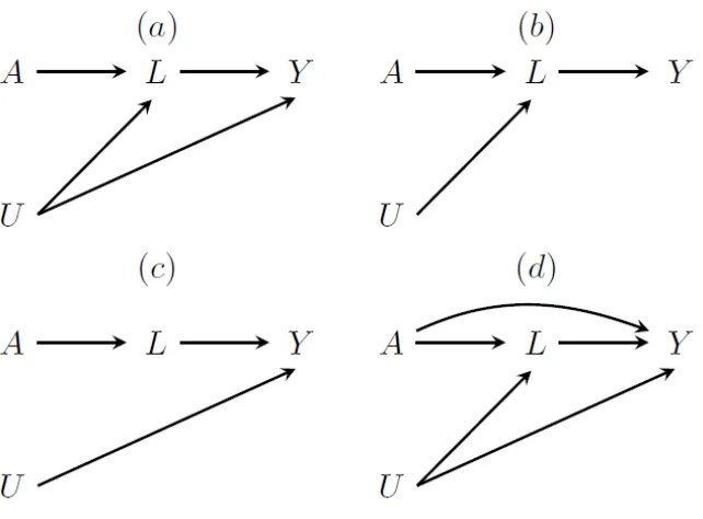
FIGURE 1.7:CAUSAL GRAPHS DEPICTING A SINGLE TIME POINT WITH TREATMENT A, OUTCOME Y, COVARIATE L, AND AN UNKNOWN VARIABLE U.THE TRUE CAUSAL EFFECT OF TREATMENT IS NON-NULL. (A)A IS A CAUSE OF Y THROUGH L ONLY, ANDUIS A CAUSE OF BOTH LAND Y;(B)A IS A CAUSE OF Y THROUGH L ONLY, AND U IS A CAUSE OF L BUT NOT
Y;(C)A IS A CAUSE OF Y THROUGH L ONLY, AND U IS A CAUSE OF Y BUT NOT L;(D)A IS A CAUSE OF Y DIRECTLY AND THROUGH L, AND U IS A CAUSE OF L AND Y. ... 33
FIGURE 2.1:SURVIVAL OVER FOLLOW-UP.(A)BASELINE FROM JAN 1,1996-DEC 31,1999,HIV-CAUSAL;(B)BASELINE FROM JAN 1,2000-DEC 31,2002,HIV-CAUSAL;(C)BASELINE ON OR AFTER JAN 1,2003,HIV-CAUSAL;(D)
BASELINE FROM JAN 1,1996-DEC 31,1999,CEPAC;(E)BASELINE FROM JAN 1,2000-DEC 31,2002,CEPAC;
(F)BASELINE ON OR AFTER JAN 1,2003,CEPAC.ALL CEPAC ESTIMATES USE 1.0 FOR MULTIPLIERS. ... 57
FIGURE 2.2:AIDS-FREE SURVIVAL OVER FOLLOW-UP.(A)BASELINE FROM JAN 1,1996-DEC 31,1999,HIV-CAUSAL;
(B)BASELINE FROM JAN 1,2000-DEC 31,2002,HIV-CAUSAL;(C)BASELINE ON OR AFTER JAN 1,2003,
HIV-CAUSAL;(D)BASELINE FROM JAN 1,1996-DEC 31,1999,CEPAC;(E)BASELINE FROM JAN 1,2000-DEC 31,
2002,CEPAC;(F)BASELINE ON OR AFTER JAN 1,2003,CEPAC.ALL CEPAC ESTIMATES USE 1.0 FOR MULTIPLIERS.
... 58
FIGURE 2.3:SURVIVAL OVER FOLLOW-UP COMPARING CEPAC CALIBRATION RUNS, WHERE MULTIPLIERS FOR OI INCIDENCE AND CHRONIC AIDS-RELATED MORTALITY ARE VARIED FROM 0 TO 1 BY 0.2,(GREY) TO HIV-CAUSAL ESTIMATES
(BLACK) WHEN BASELINE IS ON OR AFTER JAN 1,2003.(A)IMMEDIATE UNIVERSAL INITIATION;(B)INITIATION AT CD4
<500 CELLS/MM3; AND (C)INITIATION AT CD4<350 CELLS/MM3. ... 59
FIGURE 2.4:AIDS-FREE SURVIVAL OVER FOLLOW-UP COMPARING CEPAC CALIBRATION RUNS, WHERE MULTIPLIERS FOR OI INCIDENCE AND CHRONIC AIDS-RELATED MORTALITY ARE VARIED FROM 0 TO 1 BY 0.2,(GREY) TO HIV-CAUSAL ESTIMATES (BLACK) WHEN BASELINE IS ON OR AFTER JAN 1,2003.(A)IMMEDIATE UNIVERSAL INITIATION;(B)
INITIATION AT CD4<500 CELLS/MM3; AND (C)INITIATION AT CD4<350 CELLS/MM3. ... 60
vii
STRATEGY.BLACK BOX INDICATES CLOSEST MATCH TO HIV-CAUSAL ESTIMATES USING THE PARAMETRIC G-FORMULA APPLIED TO THE SUBSET WITH BASELINE ON OR AFTER JAN 1,2003; GREY BOXES INDICATE 95% CONFIDENCE
INTERVAL FOR PARAMETRIC G-FORMULA ESTIMATES USING 500 BOOTSTRAP SAMPLES. ... 61
FIGURE 2.6:7-YEAR RISK OF AIDS OR DEATH FROM CEPAC CALIBRATION RUNS BY TREATMENT STRATEGY, WHEN TREATMENT EFFECT MULTIPLIERS FOR CHRONIC AIDS-RELATED MORTALITY AND OPPORTUNISTIC INFECTIONS ARE VARIED FROM 0 TO 1.BLACK BOX INDICATES CLOSEST MATCH TO HIV-CAUSAL ESTIMATES USING THE PARAMETRIC G-FORMULA APPLIED TO THE SUBSET WITH BASELINE ON OR AFTER JAN 1,2003; GREY BOXES INDICATE 95%
CONFIDENCE INTERVAL FOR PARAMETRIC G-FORMULA ESTIMATES USING 500 BOOTSTRAP SAMPLES. ... 62
FIGURE 2.7:MEAN OF CD4 COUNT AND HIV VIRAL LOAD UNDER INTERVENTION IN CEPAC AND ESTIMATED VIA THE PARAMETRIC G-FORMULA IN HIV-CAUSALCOLLABORATION, LATE BASELINE: ON OR AFTER JAN 1,2003.ALL CEPAC ESTIMATES USE INITIAL PARAMETERIZATION OF 1.0 FOR MULTIPLIERS.(A)MEAN CD4 COUNT IN HIV-CAUSAL
(CELLS/MM3);(B)MEAN CD4 COUNT IN CEPAC(CELLS/MM3);(C)MEAN HIV VIRAL LOAD IN HIV-CAUSAL
(COPIES/ML);(E)MEAN HIV VIRAL LOAD IN CEPAC(COPIES/ML). ... 63
FIGURE 2.8:MEAN OF THE MAIN STUDY VARIABLES UNDER NO INTERVENTION: OBSERVED (SOLID LINE) AND ESTIMATED VIA THE PARAMETRIC G-FORMULA (DOTTED LINE).HIV-CAUSALCOLLABORATION, LATE BASELINE: ON OR AFTER JAN 1,
2003.(A)CUMULATIVE INCIDENCE OF DEATH;(B)CUMULATIVE INCIDENCE OF AIDS;(C)MEAN PROPORTION ON TREATMENT;(D)MEAN CD4 COUNT, NATURAL LOG SCALE;(E)MEAN HIV VIRAL LOAD. ... 82
FIGURE 2.9:MEAN OF THE MAIN STUDY VARIABLES UNDER NO INTERVENTION: OBSERVED (SOLID LINE) AND ESTIMATED VIA THE PARAMETRIC G-FORMULA (DOTTED LINE).HIV-CAUSALCOLLABORATION, INTERMEDIATE BASELINE:JAN 1,
2000–DEC 31,2002.(A)CUMULATIVE INCIDENCE OF DEATH;(B)CUMULATIVE INCIDENCE OF AIDS;(C)MEAN PROPORTION ON TREATMENT;(D)MEAN CD4 COUNT, NATURAL LOG SCALE;(E)MEAN HIV VIRAL LOAD. ... 83
viii
DEC 31,1999.(A)CUMULATIVE INCIDENCE OF DEATH;(B)CUMULATIVE INCIDENCE OF AIDS;(C)MEAN
PROPORTION ON TREATMENT;(D)MEAN CD4 COUNT, NATURAL LOG SCALE;(E)MEAN HIV VIRAL LOAD. ... 84
FIGURE 3.1:SUMMARY OF THE CEPAC DECISION PROCESS FOR DETERMINING INFECTION (I) WITH EACH OF J
OPPORTUNISTIC DISEASES IN A GIVEN MONTH K. ... 89
FIGURE 3.2:CAUSAL DIRECTED ACYCLIC GRAPH DEPICTING TWO ARBITRARY TIME POINTS FROM A SETTING WITH TIME -VARYING TREATMENT A, OUTCOME I, AND CONFOUNDER L OR CD4 COUNT, WITH AN UNMEASURED COMMON CAUSE OF CD4 COUNT AND OD INCIDENCE.CONVENTIONAL ADJUSTMENT FOR LIS EXPECTED TO INTRODUCE BIAS BECAUSE L IS AFFECTED BY PRIOR TREATMENT AND SHARES A CAUSE (U) WITH THE OUTCOME. ... 92
FIGURE 3.3:CAUSAL DIRECTED ACYCLIC GRAPH DEPICTING TWO ARBITRARY TIME POINTS FROM A SETTING WITH TIME -VARYING TREATMENT A, OUTCOME I, AND CONFOUNDER L OR CD4 COUNT IN OUR EXAMPLE, WITH AN UNMEASURED CAUSE OF CD4 COUNT ONLY. ... 95
FIGURE 3.4:CAUSAL DIRECTED ACYCLIC GRAPH DEPICTING TWO ARBITRARY TIME POINTS FROM A SETTING WITH TIME -VARYING TREATMENT A, OUTCOME I, AND CONFOUNDER L OR CD4 COUNT IN OUR EXAMPLE, WITH AN UNMEASURED CAUSE OF OD INCIDENCE ONLY. ... 96
FIGURE 3.5:MEAN OF THE MAIN STUDY VARIABLES UNDER NO INTERVENTION, WHEN FIRST DIAGNOSIS OF KAPOSI’S SARCOMA IS THE OUTCOME OF INTEREST: OBSERVED (SOLID LINE) AND ESTIMATED VIA THE PARAMETRIC G-FORMULA
(DOTTED LINE),HIV-CAUSALCOLLABORATION.(A)CUMULATIVE INCIDENCE OF KAPOSI’S SARCOMA;(B)
CUMULATIVE INCIDENCE OF DEATH;(C) MEAN PROPORTION ON TREATMENT;(D) MEAN CD4 COUNT, NATURAL LOG SCALE;(E) MEAN HIV VIRAL LOAD;(F) PROPORTION WITH AIDS-RELATED LYMPHOMA IN MONTH K;(G) PROPORTION WITH TUBERCULOSIS IN MONTH K;(H) PROPORTION WITH OTHER ODS IN MONTH K. ... 115
FIGURE 3.6:MEAN OF THE MAIN STUDY VARIABLES UNDER NO INTERVENTION, WHEN FIRST DIAGNOSIS OF AIDS-RELATED LYMPHOMA IS THE OUTCOME OF INTEREST: OBSERVED (SOLID LINE) AND ESTIMATED VIA THE PARAMETRIC G-FORMULA
ix
SCALE;(E) MEAN HIV VIRAL LOAD;(F) PROPORTION WITH KAPOSI’S SARCOMA IN MONTH K;(G) PROPORTION WITH TUBERCULOSIS IN MONTH K;(H) PROPORTION WITH OTHER ODS IN MONTH K. ... 116
FIGURE 3.7:MEAN OF THE MAIN STUDY VARIABLES UNDER NO INTERVENTION, WHEN FIRST DIAGNOSIS OF TUBERCULOSIS IS THE OUTCOME OF INTEREST: OBSERVED (SOLID LINE) AND ESTIMATED VIA THE PARAMETRIC G-FORMULA (DOTTED LINE),HIV-CAUSALCOLLABORATION.(A)CUMULATIVE INCIDENCE OF TUBERCULOSIS;(B) CUMULATIVE INCIDENCE OF DEATH;(C) MEAN PROPORTION ON TREATMENT;(D) MEAN CD4 COUNT, NATURAL LOG SCALE;(E) MEAN HIV VIRAL LOAD;(F) PROPORTION WITH KAPOSI’S SARCOMA IN MONTH K;(G) PROPORTION WITH AIDS-RELATED
LYMPHOMA IN MONTH K;(H) PROPORTION WITH OTHER ODS IN MONTH K. ... 117
x
List of Tables with Captions
TABLE 1.1:NULL TREATMENT EFFECT SIMULATION:12 MONTH RISK OF DEATH (%) ESTIMATED UNDER TWO INTERVENTIONS IN DIFFERENT SCENARIOS... 18
TABLE 1.2:HARMFUL TREATMENT EFFECT SIMULATION:12-MONTH RISK OF DEATH (%) ESTIMATED UNDER TWO
INTERVENTIONS IN DIFFERENT SCENARIOS. ... 20
TABLE 1.3:BENEFICIAL TREATMENT EFFECT SIMULATION:12-MONTH RISK OF DEATH (%) ESTIMATED UNDER TWO
INTERVENTIONS IN DIFFERENT SCENARIOS. ... 21
TABLE 1.4:SUMMARY OF POTENTIAL FOR NON-TRANSPORTABILITY AND COLLIDER BIAS IN RISK AND CAUSAL EFFECT
ESTIMATES OBTAINED BY ABMS, WHEN ONLY THE DISTRIBUTION OF U DIFFERS BETWEEN POPULATIONS. ... 27
TABLE 1.5:INPUT PARAMETERS USED TO SIMULATED OUTCOME DISTRIBUTION AND CONDITIONAL PROBABILITY
DISTRIBUTIONS OF TREATMENT AND CD4 CELL COUNT WHEN CREATING THE SIMULATED POPULATION DATA. ... 34
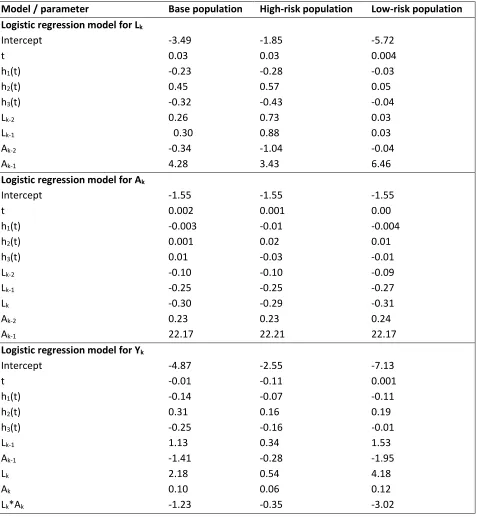
TABLE 1.6:OUTPUT PARAMETER ESTIMATES FOR LOGISTIC REGRESSION MODELS FOR TREATMENT,CD4 CELL COUNT, AND MORTALITY, BY POPULATION FOR THE NULL EFFECT SCENARIO.PARAMETERS FOR CD4 CELL COUNT AND MORTALITY MODELS USED AS INPUTS FOR PARAMETRIC G-FORMULA AND FOR THE ABMS. ... 36
TABLE 1.7:UNCERTAINTY INTERVALS FOR ABM#3 OBTAINED FROM 500 RUNS USING 1-WAY SENSITIVITY ANALYSIS OF THE EFFECT OF PAST TREATMENT ON THE OUTCOME, WHEN THE TRUE EFFECT IS NULL. ... 37
TABLE 1.8:CHECKING FOR MODEL MISSPECIFICATION: ESTIMATED MORTALITY RISK OVER FOLLOW-UP USING THE G
-FORMULA UNDER NO INTERVENTION FOR EACH POPULATION (%,95% CONFIDENCE INTERVALS). ... 38
TABLE 1.9:CHECKING FOR CONFOUNDING IN THE SIMULATED DATA: ESTIMATED DIFFERENCE IN MORTALITY RISK OVER FOLLOW-UP COMPARING ‘ALWAYS TREAT’ TO ‘NEVER TREAT’, WITHOUT ADJUSTMENT FOR THE TIME-VARYING
COVARIATE CD4 CELL COUNT (% RISK DIFFERENCE,95% CONFIDENCE INTERVALS). ... 39
TABLE 2.1:BASELINE CHARACTERISTICS OF ELIGIBLE INDIVIDUALS IN THE HIV-CAUSALCOLLABORATION BY PERIOD FOR VARIABLES USED IN CEPAC. ... 47
xi
TABLE 2.3:RISK OF ALL-CAUSE MORTALITY IN EACH BASELINE COHORT BY ART INITIATION STRATEGY,HIV-CAUSAL
COLLABORATION. ... 54
TABLE 2.4:RISK OF AIDS OR DEATH IN EACH BASELINE COHORT BY ART INITIATION STRATEGY,HIV-CAUSAL
COLLABORATION. ... 55
TABLE 2.5:DISTRIBUTION OF HIV-CAUSAL DATA BY COUNTRY OF COHORT . ... 73
TABLE 2.6:DETAILED BASELINE CHARACTERISTICS,HIV-CAUSALCOLLABORATION:EARLY BASELINE,JAN 1,1996-DEC 31,
1999. ... 74
TABLE 2.7:DETAILED BASELINE CHARACTERISTICS,HIV-CAUSALCOLLABORATION:INTERMEDIATE BASELINE,JAN 1,
2000-DEC 31,2002. ... 76
TABLE 2.8:DETAILED BASELINE CHARACTERISTICS,HIV-CAUSALCOLLABORATION:LATE BASELINE, ON OR AFTER JAN 1,
2003. ... 78
TABLE 2.9:ESTIMATED 7-YEAR RISK IN EACH BASELINE COHORT UNDER NO INTERVENTION,HIV-CAUSALCOLLABORATION.
... 80
TABLE 3.1:BASELINE CHARACTERISTICS OF ELIGIBLE INDIVIDUALS IN THE HIV-CAUSALCOLLABORATION 2003-2013. . 101
TABLE 3.2:FIRST DIAGNOSIS OF OPPORTUNISTIC DISEASES AND AIDS BY BASELINE VARIABLES,HIV-CAUSAL
COLLABORATION 2003-2013. ... 103
TABLE 3.3:BIASED ESTIMATES OF THE 1-MONTH PROBABILITY FOR FIRST DIAGNOSIS WITH EACH OD(CASES /10,000 INDIVIDUALS) BY CURRENT CD4 COUNT AND TREATMENT STATUS FROM MULTIVARIATE LOGISTIC REGRESSION WITH INDUCED COLLIDER BIAS,HIV-CAUSALCOLLABORATION 2003-2013. ... 104
xii
Acknowledgements
I would first and foremost like to acknowledge the guidance and encouragement of my doctoral
dissertation committee. Sincere thanks to my advisor, Dr. Miguel Hernán, whose patient and supportive
mentorship has been an invaluable part of my doctorate. I express my deepest gratitude for the
invaluable opportunities he has provided me to develop as a scientist and teacher, to learn, and to
advance professionally. Dr. Jamie Robins was unfailingly generous with his time and provided valuable
advice without which this dissertation would not have been possible. Dr. George Seage was encouraging
and supportive at all stages of my doctorate, and provided valuable insight into agent-based models and
HIV epidemiology for this dissertation. Dr. Ken Freedberg was extremely welcoming and open to
evaluation of the Cost-Effectiveness of AIDS Prevention model, and unfailingly positive about the
attempt to assess agent-based models from a causal inference perspective even when it seemed critical
of agent-based models.
In addition to my dissertation committee, I have had the privilege of working with and learning
from many other members of the Harvard TH Chan community. I would particularly like to thank Dr.
Paige Williams, Dr. Marcia Castro, and Dr. Marc Lipsitch for their support and advice over the past
several years. I would also like thank the members of the Causal Inference group, especially Dr. Sara
Lodi, Dr. Lauren Cain, Dr. Sonja Swanson, Dr. Xabier Garcia-De-Albeniz, Dr. Jessica Young, Dr. John
Jackson, and Dr. Roger Logan for their advice and support.
I would like to thank Mr. Richard and Mrs. Ronay Menschel for their generous funding of the
Horace W. Goldsmith Fellowship which supported me throughout my doctorate. I would also like to
thank the patients and providers in the HIV-CAUSAL Collaboration without whom the analyses in
xiii
I would especially like to thank my fellow students at Harvard Chan. To my qualifying exam
study group, Kirsten Dorans, Emilie Zoltick, and Amy Shafrir, thank you for your friendship and support
for the past 5 years and for making me a better epidemiologist. To Rachel Zack, Iris Kim, Claire Pernar,
Leslie Farland, Corey Peak, Justin Bohn, and Patrick Mitchell, thank you for all the laughs, and for not
laughing too loud when I ask a ridiculous question.
To Carly Hughes and Ellie Caniglia, I would like to express my deepest thanks—you are the best
and I can’t imagine how different the past several years would have been without you, and your
unfailing support, advice, and encouragement of everything from research problems to coffee breaks.
You made the lowlights into highlights!
Finally, thank you to my family, and to my partner, Kareem, who have been unfailingly
supportive of my many, many years of education. I am forever grateful for their love and
encouragement. They give me courage to reach for my goals and push me to aim high. To my three
nieces and my nephew, all of whom were born during my doctorate, your smiling faces always improve
my day and I love you to pieces.
1
Introduction
Sound clinical decision making requires estimating the outcome distribution under different
treatment strategies. In the absence of randomized trials, two possible approaches are agent-based
models (ABM) and the parametric g-formula. Though mathematically similar, these methods have
generally been considered in isolation. In this dissertation, we bridge the gap between ABMs and the
parametric g-formula, and provide recommendations to use ABMs for causal inference.
In Chapter 1, we describe a previously unrecognized bias that can occur when extrapolating
ABM estimates to a population different from the one that was used to construct the model. The bias
will occur when the outcome and time-varying confounders of the treatment-outcome relationship
share causes, and the conditional association between treatment and outcome is endowed with an
unwarranted causal interpretation. We demonstrate the impact of this bias by comparing estimates
from the parametric g-formula and several versions of an ABM in simulated data. We discuss the
conditions required for unbiased results.
In Chapter 2, we describe an approach to provide calibration targets for ABMs, and to identify
the set of parameters of the ABM that interfere with transportability of the model results to a particular
population. We illustrate this approach by comparing the 7-year mortality estimated by an existing
ABM, the Cost-Effectiveness of Preventing AIDS Complications (CEPAC) model, to estimates from the
parametric g-formula applied to a prospective clinical data from 60178 HIV-positive individuals under
different treatment initiation strategies. The CEPAC estimates were most sensitive to associational
parameters interpreted causally as the effect of treatment on opportunistic infections and chronic
AIDS-related mortality. Changes to these parameters eliminated the discrepancies between CEPAC and
2
In Chapter 3, we focus on the core problem of causal inference from ABMs: how to define and
estimate the parameters described in Chapter 2 in light of the bias described in Chapter 1. To illustrate
this problem, we consider CEPAC input parameters for opportunistic diseases—namely, the 1-month
probabilities of each opportunistic disease, conditional on current CD4 count and the multiplier of these
probabilities under treatment. We formally define the effect of interest for these inputs and describe
the conditions under which this effect is or is not identifiable. We then describe the assumptions
required to allow transportability of this effect between populations. Finally, we show that the
3
Chapter 1
A comparison of agent-based models and the parametric g-formula
for causal inference
Eleanor J. Murray1, James M. Robins1,2, George R. Seage III1, Kenneth A. Freedberg3,4,5, Miguel A. Hernán1,2,6
Affiliations
1Department of Epidemiology, Harvard T.H. Chan School of Public Health, Boston, MA
2Department of Biostatistics, Harvard T.H. Chan School of Public Health, Boston, MA
3Department of Medicine, Massachusetts General Hospital, Boston, MA
4Department of Health Policy and Management, Harvard T.H. Chan School of Public Health, Boston, MA
5Center for AIDS Research, Harvard University, Boston, MA
4
ABSTRACT
Medical decision making requires choosing from treatment strategies on the basis of correctly
estimated outcome distributions. In the absence of randomized trials, two possible approaches are
agent-based models (ABMs) and the parametric g-formula. Validity of the g-formula requires strong
assumptions, and is limited to the population from which data were collected. ABMs are used to
estimate effects across populations, but rely on assumptions that are generally even stronger;
substantial bias can arise when these are incorrect. We describe potential biases when using ABMs for
causal inference. We estimated 12-month mortality, using an ABM and the parametric g-formula, in
three simulated populations differing only in the prevalence of an unknown common cause of mortality
and a known time-varying confounder. The g-formula and ABM correctly estimated mortality when all
inputs came directly from the population of interest. The ABM was biased when any inputs came from
another population. Both methods can afford to ignore unmeasured determinants of the outcome when
causal inference is restricted to a population with sufficient data on confounders, treatment, and
outcome. However, the use of ABMs for causal inferences on another population may be biased even if
5
INTRODUCTION
Medical decision making requires choices among treatment strategies. For these decisions to be
sound, researchers need to correctly estimate the distribution of the outcome—survival,
cost-effectiveness, or another utility function—under each of the candidate strategies. When a randomized
controlled trial of these strategies is not feasible, two possible approaches for estimating the impact of
candidate treatment strategies are agent-based, or individual-level, models (ABMs) 1,2, and the
parametric g-formula 3,4.
ABMs and the parametric g-formula use a similar mathematical approach: construction of a
sequential model which is the basis of a Monte Carlo simulation of a (counterfactual) population under
each treatment strategy of interest. However, despite the shared approach and goals, ABMs and the
parametric g-formula have generally been considered in isolation and there is typically little overlap in
the population of researchers familiar with each method 5,6.
To construct the sequential model, ABMs typically combine data from multiple sources, whereas
applications of the parametric g-formula use data from a single prospective study. As a result, inferences
from the parametric g-formula tend to be restricted to populations similar to the study population and
to the time horizon and treatment strategies that are observed in the data. In contrast, ABMs are
generally seen as a tool to address questions that are not constrained by the population characteristics,
time horizon, and treatment strategies observed in any particular study 7.
The greater flexibility of ABMs comes at a price: for the extrapolations to be correct, the model
needs to make implicit or explicit assumptions about variables that remain unmeasured in most human
studies. In contrast, the parametric g-formula is agnostic about the distribution of those unmeasured
6
implies that the input parameters of ABMs are implicitly endowed with a causal interpretation whereas
the input parameters of the parametric g-formula quantify statistical associations that may or may not
have a causal interpretation. In other words, ABMs use causal models to yield causal estimates that can
be extrapolated to many populations, whereas the parametric g-formula uses non-causal models to
yield causal estimates in a single population 3,4.
In this paper we explore the practical consequences of this divergent interpretation of the
model parameters between ABMs and the parametric g-formula. We start with the description of a
simplified decision analysis example; the goal is to determine whether we can improve the 12-month
survival of HIV-positive individuals by offering them antiretroviral therapy.
A SIMPLIFIED DECISION ANALYSIS EXAMPLE
Let Akbe an indicator for initiation of antiretroviral treatment in month k,Lk an indicator for high
CD4 cell count (defined as ≥350 cells/μl) measured at the beginning of month k, and Yk+1 an indicator for death by the beginning of month k+1. We use overbars to represent history. For example, an individual with a high CD4 cell count in months 1 and 2, and low in month 3, has CD4 count history 𝐿𝐿�3 =(1,1,0).
As shown in the decision tree 1,8 depicted in Figure 1.1, a decision to start treatment is more
likely when previous CD4 cell counts are low, which indicates a worse prognosis 9. Therefore an
individual’s probability of initiating treatment at k, Pr(𝐴𝐴𝑘𝑘= 1|𝐿𝐿�𝑘𝑘,𝐴𝐴𝑘𝑘−1 = 0,𝑌𝑌�𝑘𝑘 = 0), depends on her CD4 cell count history and possibly her treatment history. Once initiated, treatment is maintained until
death. The probabilities of having a low CD4 cell count, Pr(𝐿𝐿𝑘𝑘 = 1|𝐿𝐿�𝑘𝑘−1,𝐴𝐴̅𝑘𝑘−1,𝑌𝑌�𝑘𝑘 = 0), and of
7
Figure 1.1: Simplified decision process for the use of treatment among HIV-positive individuals at each month k. Square black nodes represent decision points where intervention is possible, white circles represent nodes where an individual’s path depends on the conditional probability distribution specified, triangles represent terminal nodes.
Suppose we are interested in the effect of treatment on 1-year mortality risk. We might specify
treatment strategies, such as ‘always treat’ and ‘never treat’. We can then create an ABM where
treatment at each time point is assigned based on one of these strategies and compare the
(counterfactual) 1-year mortality risk under each. Similarly, we can use the parametric g-formula to
estimate these mortality risks.
Agent-based model
8
probabilities Pr(𝐿𝐿𝑘𝑘 = 1|𝐿𝐿�𝑘𝑘−1,𝐴𝐴̅𝑘𝑘−1,𝑌𝑌�𝑘𝑘 = 0) and Pr(𝑌𝑌𝑘𝑘+1= 1|𝐿𝐿�𝑘𝑘,𝐴𝐴̅𝑘𝑘,𝑌𝑌�𝑘𝑘 = 0) govern movement
between states conditional on prior history. These probabilities are obtained from published sources,
including randomized trials and observational studies 10. The dependence of these probabilities on prior
history is often achieved through modeling. For example, a model for the monthly conditional
probability of mortality may be logit Pr(𝑌𝑌𝑘𝑘+1= 1|𝐿𝐿�𝑘𝑘,𝐴𝐴̅𝑘𝑘,𝑌𝑌�𝑘𝑘 = 0) = 𝛽𝛽0+𝛽𝛽1ℎ(𝑡𝑡) +𝛽𝛽2𝐿𝐿𝑘𝑘+𝛽𝛽3𝐿𝐿𝑘𝑘−1+
𝛽𝛽4𝐴𝐴𝑘𝑘+𝛽𝛽5𝐴𝐴𝑘𝑘−1+𝛽𝛽6(𝐿𝐿𝑘𝑘×𝐴𝐴𝑘𝑘) , where h(t) is a flexible function (e.g., restricted cubic splines) of time k, and the vector of parameters β is replaced by estimates from a similar model fit to observational data in the literature. Similarly, a model for the monthly conditional probability of high CD4 cell count may
be logit Pr(𝐿𝐿𝑘𝑘 = 1|𝐿𝐿�𝑘𝑘−1,𝐴𝐴̅𝑘𝑘−1,𝑌𝑌�𝑘𝑘 = 0) = 𝛾𝛾0+𝛾𝛾1ℎ(𝑡𝑡) +𝛾𝛾2𝐿𝐿𝑘𝑘−1+𝛾𝛾3𝐿𝐿𝑘𝑘−2+𝛾𝛾4𝐴𝐴𝑘𝑘−1+𝛾𝛾5𝐴𝐴𝑘𝑘−2 ,
where the vector of estimated parameters is also obtained from one or more observational studies or
randomized trials.
Investigators then use these models to simulate individuals’ trajectories under a strategy of
interest. For example, if interested in comparing the 1-year mortality risk under the strategies “always
treat” and “never treat,” we would set the conditional probability for initiating treatment Pr(𝐴𝐴𝑘𝑘=
1|𝐿𝐿�𝑘𝑘,𝐴𝐴̅𝑘𝑘−1,𝑌𝑌�𝑘𝑘 = 0) = 1 for the first time point and conduct a Monte Carlo simulation 1 with 1,000,000
individuals, and, separately, set the conditional probabilities Pr(𝐴𝐴𝑘𝑘 = 1|𝐿𝐿�𝑘𝑘,𝐴𝐴̅𝑘𝑘−1,𝑌𝑌�𝑘𝑘 = 0) = 0 for all k and conduct another Monte Carlo simulation. The 1-year mortality risks estimated from these
simulations would then be compared.
The parametric g-formula
The implementation of the parametric g-formula 3,4,11 has the same two steps as that of ABMs:
specification of parametric models for Pr(𝐿𝐿𝑘𝑘 = 1|𝐿𝐿�𝑘𝑘−1,𝐴𝐴̅𝑘𝑘−1,𝑌𝑌�𝑘𝑘 = 0) and Pr(𝑌𝑌𝑘𝑘+1= 1|𝐿𝐿�𝑘𝑘,𝐴𝐴̅𝑘𝑘,𝑌𝑌�𝑘𝑘 = 0),
followed by Monte Carlo simulation under the treatment strategies of interest. The parameters of these
9
monthly measurements of CD4 cell count, treatment, and mortality. As long as data are available on all
variables in the model, the parametric g-formula could be based on exactly the same parametric models
that define the ABM.
Because of the dependence on observed data, parametric g-formula users tend to restrict their
inferences to settings, populations, and time frames similar to those of the study population. In contrast,
ABM users routinely make inferences across settings, populations, and time frames. This extrapolation
generally requires that the model parameters are interpreted as causal effects. This causal
interpretation, which is not necessary for the more modest aims of the parametric-g-formula, is
problematic when treatment-confounder feedback exists, as we explain in the next section.
TREATMENT-CONFOUNDER FEEDBACK
The causal diagram in Figure 1.2 represents two time points for the setting described in the
previous sections. We say that there is treatment-confounder feedback because, at each time point k, confounder CD4 cell count Lk affects subsequent treatment Ak and is affected by prior treatment Ak-1. The causal diagram also includes an unmeasured prognostic factor U which independently affects both the confounder CD4 cell count and the mortality outcome. Unmeasured common causes of confounders
10
Figure 1.2: Causal directed acyclic graph depicting two arbitrary time points from a setting with time-varying treatment A, outcome Y, and confounder L. Conventional adjustment for L is expected to introduce bias because L is affected by prior treatment and shares a cause (U) with the outcome.
The simultaneous presence of treatment-confounder feedback and the unmeasured U is the main reason why conventional outcome regression cannot be generally used to estimate the
counterfactual probability under the treatment strategies of interest. Since an outcome regression
model needs to include Lk as a covariate to adjust for confounding for the effect of Ak on Yk, the method estimates the probability of the outcome Yk conditional on Lk. However, because Lk is a collider (a common effect of two variables) on the path from Ak-1 to Yk and conditioning on a collider will generally induce an association between its causes 12, conditioning on Lk would create an association between Ak-1 and U, and therefore between Ak-1 and Yk (because U is associated with Yk).
As an example, consider the outcome regression model for logit Pr(𝑌𝑌𝑘𝑘+1 = 1|𝐿𝐿�𝑘𝑘,𝐴𝐴̅𝑘𝑘,𝑌𝑌�𝑘𝑘=
0) described in the previous section. The parameter β5 for past treatment quantifies the conditional
association between Ak-1 and Yk. Part of this association may be due to the direct causal effect on Ak-1 on Yk that is not mediated through Lk and the other variables in the model, and another part of this
11
interpreted causally as the direct effect of past treatment that is not mediated through the other
variables in the model.
The impossibility to endow the parameter β5 with a causal interpretation is not a problem for
the parametric g-formula, which simply uses the models for Pr(𝐿𝐿𝑘𝑘 = 1|𝐿𝐿�𝑘𝑘−1,𝐴𝐴̅𝑘𝑘−1,𝑌𝑌�𝑘𝑘 = 0) and
Pr(𝑌𝑌𝑘𝑘+1 = 1|𝐿𝐿�𝑘𝑘,𝐴𝐴̅𝑘𝑘,𝑌𝑌�𝑘𝑘 = 0) as an intermediate step to estimate the counterfactual probability of death
in the study population 3,4. ABMs, on the other hand, endow individual model parameters with a causal
interpretation to allow for extrapolation. Thus the parameter β5 in the outcome model of the ABM is
interpreted as the direct effect of Ak-1 on Yk. Unfortunately, such an effect cannot be estimated without bias in the presence of an unmeasured common cause U.
In the next sections, we summarize the sources of bias (including treatment-confounder
feedback) for ABMs constructed using data from certain populations when making inferences for other
populations.
BIAS EVEN IF THE ABM IS BASED ON DATA FROM A PERFECT RANDOMIZED TRIAL
ABM estimates may be biased even if the model is parametrized using data from a perfect
randomized trial. To show this, we further simplify our example to treatment decisions (A0, A1) at two
times only.
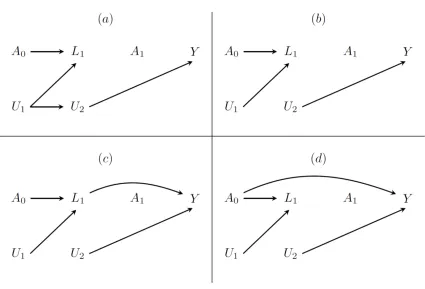
Suppose we have data on A0, A1, L1 and Y from a perfect randomized trial with four arms: (A0 =0,
A1=0), (A0 =0, A1=1), (A0 =1, A1=0), and (A0 =1, A1=1). Suppose that Figure 1.3(a) depicts the true but
unknown causal graph. Because the distribution of Y does not depend on A0 and A1, a regression of Y on
A0 and A1 that ignores data on L1 (as well as a g-formula analysis that uses data on L1) will correctly
estimate the null causal effects of A0 and A1 on Y. Similarly, a regression of L1 on A0 will correctly
12
association, which is a biased estimate of the null causal effect of L1 on Y because of unmeasured
confounding by the path L1 ←U1→U2 →Y, and a regression of Y on A0, A1, L1 will yield a non-null A0 -Y
association, which is a biased estimate of the null causal effect of A0 on Y because L1 is a collider on the
[image:26.612.89.514.188.477.2]path from A0 to Y.
Figure 1.3: Causal directed acyclic graphs depicting four scenarios for an ideal randomized trial to estimate the effect of treatment A0 on L1 and the joint effect of treatments A0 and A1 on Y. U1 and U2
are unmeasured variables.
Now consider an ABM researcher who wants to use trial estimates and then transport them to a
new population in which distribution of U1 is the same as in the trial, but the conditional distributions of
U2 given U1 and Y given U2 are not. He believes that he can use regressions from the trial to estimate the
effects of A0 on L1, of A0, A1 on L1, and of L1 on Y. Suppose that the researcher finds that the A0 -L1
13
even more certain the trial can be used to parametrize his ABM. However, as we have discussed, an
ABM using parameters estimated from the perfect trial will falsely find a causal effect of A0 on Y.
Now suppose that Figure 1.3(b) depicts the true causal graph, in which there is no arrow from U1
to U2. Because now there is no L1-Y confounding and no A0 -Y association conditional on L1, the
regression of Y on A0, A1, and L1 in the trial data will correctly estimate the null causal effects of A0, A1,
and L1 on Y. In this case, the ABM will correctly show no effect of A0 and A1 on Y. However, because the
marginal distribution of U2 and the conditional distribution of Y given U2 differ between the trial
population and the new population, the marginal distribution of Y from the new population data and
that computed under any strategy using the ABM will be different. That is, the marginal distribution of Y
is non-transportable from the trial to the new population, as can be seen from the graphical results of
Bareinboim and Pearl 13,14 or directly from the g-formula (Appendix 1).
Suppose, we still have the U1 to U2 arrow missing but now the marginal distribution of U2 and
the conditional distribution of Y given U2 are the same between the trial and the new population, but
the marginal distribution of U1 and the conditional distribution of L1 given A0 and U1 are different
between these populations. Then, the law of L1 given A0 (and thus the causal effect of A0 on L1) will now
differ between the trial and the new population, but the ABM will correctly show no effect of A0 and A1
on Y in the new population, and the marginal distribution of Y will be transportable from the trial to the
new population.
Next suppose that the true causal graph has an arrow from L1 to Y (Figure 1.3(c)) or from A0 to Y
(Figure 1.3(d)) so that A0 has an effect on Y. Then, even in the absence of confounding (i.e., no U1 to U2
arrow), the magnitude of the causal effects of A0 and A1 on Y in the new population will differ from that
14
biased estimate given by the ABM of the effect in the new population. This again follows from the
graphical results of Bareinboim and Pearl 13,14 or directly from the g-formula (Appendix 1).
The next section describes a simulation study that quantifies these biases in our example with
multiple treatment decisions over time.
SIMULATIONS UNDER A NULL TREATMENT EFFECT
Simulation scenarios
We simulated three scenarios: a base scenario with approximately 10% mortality at 12 months,
a high-risk scenario with approximately 50% mortality, and a low-risk scenario with approximately 1%
mortality. For each scenario, we simulated a cohort of 106 HIV-positive individuals followed for 12
months under the data generating mechanism depicted in Figure 1.2. We simulated the monthly CD4
count, treatment, and death status, with no missing data, for each individual. Treatment had a null
effect on mortality, which could represent the comparison of two active treatments of equal
effectiveness, or the comparison of an ineffective treatment with no treatment.
In each scenario, we estimate the counterfactual 12-month mortality risk under the two
treatment strategies “always treat” and “never treat”. We first estimated these risks using the
parametric g-formula applied to the simulated data. We then estimated these risks using ABMs with the
same model specification as the parametric g-formula.
In the high- and low-risk scenarios, we implemented four types of ABMs depending on the origin
of the model parameters:
1. The scenario of interest (high- or low-risk). This ABM #1 is expected to provide an unbiased
15
2. The base scenario. This ABM #2 is expected to provide a mortality estimate that is unbiased
for the base scenario but biased for the high- and low-risk scenarios, because of non-transportability.
3. The parameter for prior treatment β5 from the base scenario and all other parameters from
the scenario of interest. This ABM #3 is expected to provide a biased mortality estimate because the
magnitude of the association between prior treatment and the outcome conditional on a collider
generally varies across populations with different outcome risk.
4. The parameter for prior treatment β5 from the scenario of interest, and all other parameters
from the base scenario. This ABM #4 is subject to the two sources of bias in 2. and 3. above.
The data were simulated following the algorithm described by Robins 15 and Young et al 16
(Appendix 2). SAS 9.4 was used for all analyses.
Estimation via the parametric g-formula
Let g represent a treatment strategy for k= 0,…K months of follow-up,𝑌𝑌𝑘𝑘+1𝑔𝑔 the counterfactual value for an individual’s outcome if she had followed strategy g, and 𝑎𝑎�𝑘𝑘𝑔𝑔 a treatment history up to month k that is consistent with the strategy g. For example, for the strategy “always treat”, 𝑎𝑎�𝑘𝑘𝑔𝑔= (a0 = 1, a1 = 1, …, ak = 1). Our goal is to estimate the counterfactual mortality risk under a strategy g by time k+1, that is, Pr(Ygk+1=1). Under the decision process in Figure 1.1 (equivalent to the data generation mechanism in
Figure 1.2), this counterfactual risk is equal to the g-formula 17:
=� �Pr�𝑌𝑌𝑗𝑗+1= 1|𝐿𝐿�𝑗𝑗=𝑙𝑙̅𝑗𝑗,𝐴𝐴̅𝑗𝑗 =𝑎𝑎�𝑗𝑗𝑔𝑔,𝑌𝑌�𝑗𝑗= 0� 𝑘𝑘
𝑗𝑗=0
𝑙𝑙̅𝑘𝑘
×� �𝑃𝑃𝑃𝑃�𝑌𝑌𝑠𝑠= 0|𝐿𝐿�𝑠𝑠−1=𝑙𝑙̅𝑠𝑠−1,𝐴𝐴̅𝑠𝑠−1=𝑎𝑎�𝑠𝑠−1𝑔𝑔 ,𝑌𝑌�𝑠𝑠−1= 0�×𝑓𝑓�𝑙𝑙𝑠𝑠|𝑙𝑙̅𝑠𝑠−1,𝑎𝑎�𝑠𝑠−1𝑔𝑔 ,𝑌𝑌�𝑠𝑠−1= 0�� 𝑗𝑗
16
We estimated the factors of the g-formula via the parametric 𝑙𝑙𝑙𝑙𝑙𝑙𝑙𝑙𝑡𝑡Pr(𝐿𝐿𝑘𝑘 = 1|𝐿𝐿�𝑘𝑘−1 =
𝑙𝑙̅𝑘𝑘−1, 𝐴𝐴̅𝑘𝑘−1=𝑎𝑎�𝑘𝑘−1, 𝑌𝑌�𝑘𝑘 = 0) = 𝛾𝛾0+𝛾𝛾1𝑡𝑡+𝛾𝛾2ℎ1(𝑡𝑡) +𝛾𝛾3ℎ2(𝑡𝑡) +𝛾𝛾4ℎ3(𝑡𝑡) +𝛾𝛾5𝐿𝐿𝑘𝑘−2+𝛾𝛾6𝐿𝐿𝑘𝑘−1+
𝛾𝛾7𝐴𝐴𝑘𝑘−2+𝛾𝛾8𝐴𝐴𝑘𝑘−1, and 𝑙𝑙𝑙𝑙𝑙𝑙𝑙𝑙𝑡𝑡Pr(𝑌𝑌𝑘𝑘+1= 1|𝐿𝐿�𝑘𝑘, 𝐴𝐴̅𝑘𝑘, 𝑌𝑌�𝑘𝑘 = 0) = 𝛽𝛽0+𝛽𝛽1𝑡𝑡+𝛽𝛽2ℎ1(𝑡𝑡) +𝛽𝛽3ℎ2(𝑡𝑡) +
𝛽𝛽4ℎ3(𝑡𝑡) +𝛽𝛽5𝐴𝐴𝑘𝑘−1+𝛽𝛽6𝐴𝐴𝑘𝑘+𝛽𝛽7𝐿𝐿𝑘𝑘−1+𝛽𝛽8𝐿𝐿𝑘𝑘+𝛽𝛽9(𝐿𝐿𝑘𝑘𝐴𝐴𝑘𝑘), where, hj(t) represents restricted cubic splines with knots at 3, 6, 9 and 12 months (Technical Appendix Table 1.6). We approximated the sum
through a Monte-Carlo simulation of 106 individuals under the strategy g of interest (the value of Ak at every month was assigned as 1 or 0 for the interventions ‘always treat’ and ‘never treat’, respectively).
95% confidence intervals were obtained via 500 bootstrap samples.
We used a SAS macro to get the parametric g-formula estimates 18. The macro is available at
http://www.hsph.harvard.edu/causal/software/
Estimation via the ABM
The algorithm for estimating the ABM is similar to that for the g-formula, except for the source
of parameters for the conditional distributions of Y and L. The parameters estimated for each simulated population are given in Technical Appendix Table 1.6. The inputs to the ABMs were chosen from these
estimates, based on the appropriate source for each ABM type and scenario. The conditional probability
models used for the ABMs were identical to those specified above for the parametric g-formula. For all
scenarios, the baseline confounder distribution was estimated from the corresponding empirical
distribution. To reduce the impact of stochastic noise, we used the same set of random seeds to
17
Simulation results
The first row of Table 1.1 shows the 12-month mortality risk in the 3 simulated scenarios.
The next two rows show estimates under ‘always treat’ and ‘never treat’ for the parametric
g-formula and ABM #1. As expected, both methods estimated identical risks. Table 1.1 shows the 95%
confidence intervals around the g-formula estimates. See Appendix 4 for uncertainty intervals around
the ABM estimates 19. Although the uncertainty intervals obtained from these sensitivity analyses are
not interpretable as confidence intervals, they can provide some insight into the range of possible
outcome distributions consistent with variations of the model 20.
The next rows of Table 1.1 show estimates for ABMs #2, #3, and #4 for the high- and low-risk
scenarios. ABM #2 predictably replicates the g-formula estimates from the base scenario and the risk
estimates are therefore biased for the high- and low-risk scenarios. However, since the effect is null in
all populations, the causal effect estimate from ABM #2 is correct for the high- and low-risk scenarios.
18
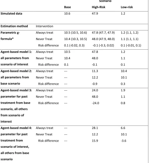
Table 1.1: Null treatment effect simulation: 12 month risk of death (%) estimated under two interventions in different scenarios.
Scenario
Base High-Risk Low-risk
Simulated data 10.6 47.9 1.2
Estimation method Intervention
Parametric g-formula*
Always treat 10.5 (10.5, 10.6) 47.8 (47.7, 47.9) 1.2 (1.1, 1.2)
Never Treat 10.4 (10.3, 10.5) 48.0 (47.9, 48.0) 1.1 (1.1, 1.1)
Risk difference 0.1 (-0.02, 0.3) -0.1 (-0.3, 0.02) 0.1 (-0.01, 0.1)
Agent-based model 1: all parameters from scenario of interest
Always treat 10.5 47.8 1.2
Never Treat 10.4 48.0 1.1
Risk difference 0.1 -0.1 0.1
Agent-based model 2: all parameters from base scenario
Always treat --- 11.3 10.4
Never Treat --- 12.2 10.1
Risk difference --- -0.9 0.3
Agent-based model 3: parameter for past treatment from base scenario, all others from scenario of interest
Always treat --- 24.0 1.9
Never Treat --- 48.0 1.1
Risk difference --- -24.0 0.8
Agent-based model 4: parameter for past treatment from scenario of interest, all others from base scenario
Always treat --- 28.1 6.6
Never Treat --- 12.2 10.1
Risk difference --- 15.9 -3.6
19
SIMULATIONS UNDER A NON-NULL TREATMENT EFFECT
Simulation scenarios
We conducted two additional sets of simulations that were identical to the one described above
except that the treatment effects were non-null. In one, treatment was designed to have a harmful
effect on survival, with treated individuals expected to have a mortality rate approximately twice as high
as untreated individuals. In the second, treatment was designed to have a beneficial effect on survival,
such that individuals who were treated were expected to have a mortality rate approximately half that
of individuals who were untreated.
Simulation results
When the treatment was harmful, 12-month mortality increased in all scenarios (Table 1.2). As
expected, ABM #2 replicated the base scenario 12-month mortality. However, since the treatment effect
was no longer null, the causal effect estimates from ABM #2 were no longer unbiased for the
populations of interest. ABMs #3 and #4 were biased for both the high- and low-risk scenarios. The
direction and magnitude of the bias varied between simulations.
When the treatment was protective, 12-month mortality decreased in all scenarios (Table 1.3).
Again, ABM #2 replicated the base-case scenario, although less closely than with a null treatment effect,
and the casual effect estimate was biased for both the high- and low-risk populations. ABM #3 and ABM
20
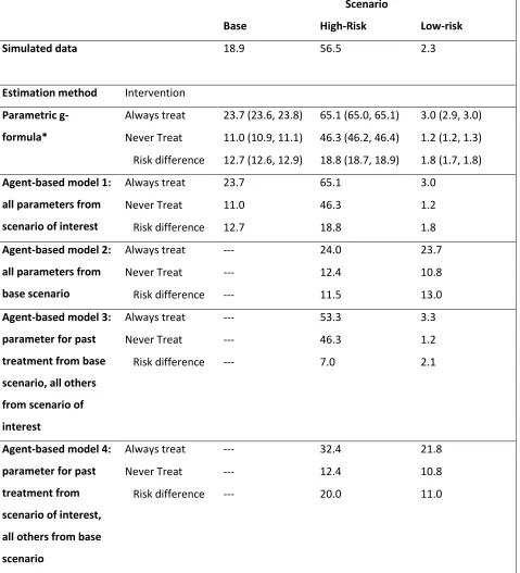
Table 1.2: Harmful treatment effect simulation: 12-month risk of death (%) estimated under two interventions in different scenarios.
Scenario
Base High-Risk Low-risk
Simulated data 18.9 56.5 2.3
Estimation method Intervention
Parametric g-formula*
Always treat 23.7 (23.6, 23.8) 65.1 (65.0, 65.1) 3.0 (2.9, 3.0)
Never Treat 11.0 (10.9, 11.1) 46.3 (46.2, 46.4) 1.2 (1.2, 1.3)
Risk difference 12.7 (12.6, 12.9) 18.8 (18.7, 18.9) 1.8 (1.7, 1.8)
Agent-based model 1: all parameters from scenario of interest
Always treat 23.7 65.1 3.0
Never Treat 11.0 46.3 1.2
Risk difference 12.7 18.8 1.8
Agent-based model 2: all parameters from base scenario
Always treat --- 24.0 23.7
Never Treat --- 12.4 10.8
Risk difference --- 11.5 13.0
Agent-based model 3: parameter for past treatment from base scenario, all others from scenario of interest
Always treat --- 53.3 3.3
Never Treat --- 46.3 1.2
Risk difference --- 7.0 2.1
Agent-based model 4: parameter for past treatment from scenario of interest, all others from base scenario
Always treat --- 32.4 21.8
Never Treat --- 12.4 10.8
Risk difference --- 20.0 11.0
21
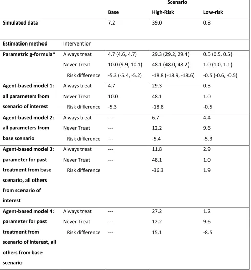
Table 1.3: Beneficial treatment effect simulation: 12-month risk of death (%) estimated under two interventions in different scenarios.
Scenario
Base High-Risk Low-risk
Simulated data 7.2 39.0 0.8
Estimation method Intervention
Parametric g-formula* Always treat 4.7 (4.6, 4.7) 29.3 (29.2, 29.4) 0.5 (0.5, 0.5)
Never Treat 10.0 (9.9, 10.1) 48.1 (48.0, 48.2) 1.0 (1.0, 1.1)
Risk difference -5.3 (-5.4, -5.2) -18.8 (-18.9, -18.6) -0.5 (-0.6, -0.5)
Agent-based model 1: all parameters from scenario of interest
Always treat 4.7 29.3 0.5
Never Treat 10.0 48.1 1.0
Risk difference -5.3 -18.8 -0.5
Agent-based model 2: all parameters from base scenario
Always treat --- 6.7 4.4
Never Treat --- 12.2 9.6
Risk difference --- -5.4 -5.3
Agent-based model 3: parameter for past treatment from base scenario, all others from scenario of interest
Always treat --- 11.8 2.9
Never Treat --- 48.1 1.0
Risk difference -36.3 1.9
Agent-based model 4: parameter for past treatment from scenario of interest, all others from base scenario
Always treat --- 27.2 1.2
Never Treat --- 12.2 9.6
Risk difference --- 15.1 -8.5
22
DISCUSSION
In our simplified example, mortality risk was always correctly estimated when model parameters
were estimated from the same population to which the model was applied, regardless of whether we
used the parametric g-formula or an ABM. In our example, the ABM and the parametric g-formula are
mathematically identical when the parameters of both are estimated from the population of interest.
However, mortality risks were biased when parameters of ABMs were obtained from populations other
than the target population. Bias arose even if the causal structure and magnitude of treatment effects
were constant across populations. The bias has two distinct sources: 1) differences in distributions of
unmeasured risk factors between populations and 2) use of models that require knowledge about the
conditional association between treatment and outcome conditional on colliders.
The first source of bias was demonstrated by ABM #2, which was parameterized using
parameters from the base-case scenario and therefore did not provide accurate mortality estimates in
the high- and low-risk scenarios. This bias reflects the expected lack of transportability 13,14. The second
source of bias was demonstrated by ABM #3, in which the only parameter not estimated in the target
population was the association between past treatment and the outcome conditional on confounders
for subsequent treatment that were affected by both past treatment and unmeasured determinants of
the outcome. This bias is expected, even under the null, because of collider stratification. If the true
effect of treatment is non-null, bias can arise even when U is associated with only one of Lk or Yk (see Appendix Section 1 for details). Our ABM #4 combined both sources of bias.
To avoid these biases, modelers might consider one of the following three strategies when
23
First, the ABM can be parameterized based on studies in which confounding by common causes
of variables affected by treatment and of the outcome has been appropriately adjusted for. In our
example, this strategy requires that some studies have unbiasedly estimated the effects of treatment
and CD4 count on death, and the effects of past treatment on CD4 count and of CD4 count on
treatment. Unfortunately, unbiased estimation of the effects of past treatment and CD4 count requires
adjustment for confounding by common causes like the variable U, which are generally unavailable to analysts.
Second, the ABM can incorporate all (measured and unmeasured) determinants of the outcome
in the ABM. In our example, the ABM would need to include the unmeasured variable U. Unfortunately, many of these determinants will be either unknown or unmeasured due to technical or resource
limitations. Even if they were measured, it would be challenging to find parameter estimates from all
components of a model that is now conditioned on generally unavailable variables.
Third, the ABM can be parameterized using parameter estimates from populations where the
distribution of risk factors, including these common causes, is known to be identical to that in the
population of interest. Unfortunately, this would severely limit the applicability of the model.
Given the difficulty of implementing the above strategies, a more realistic course of action may
be design of sensitivity analyses on parameters that measure the association between treatment and
outcome conditional on variables affected by treatment.
In summary, both the parametric g-formula and ABMs can afford to ignore unmeasured
determinants of the outcome when causal inference is restricted to a population with sufficient data on
confounders, treatment, and outcome. However, the use of ABMs for causal inferences on another
24
ACKNOWLEDGEMENTS
This work was supported in part by the National Institutes of Health (Grant R01-AI073127 to M.
25
REFERENCES
1. Sonnenberg FA, Beck JR. Markov models in medical decision making: a practical guide. Medical
Decision Making 1993;13(4):322-38.
2. Beck JR, Pauker SG. The Markov process in medical prognosis. Medical Decision Making
1983;3(4):419-458.
3. Robins JM, Hernán MA. Estimation of the causal effects of time-varying exposures. In: Fitzmaurice G, Davidian M, Verbeke G, Molenberghs G, eds. Longitudinal Data Analysis. New York: Chapman and Hall/CRC Press, 2008;553-599.
4. Robins J. A new approach to causal inference in mortality studies with sustained exposure periods - Application to control of the healthy worker survivor effect. Mathematical Modelling 1986;7:1396-1512.
5. Marshall BDL, Galea S. Formalizing the role of agent-based modeling in causal inference and epidemiology. American Journal of Epidemiology 2015;181(2):92-99.
6. Hernán MA. Invited commentary: Agent-based models for causal inference-reweighting data
and theory in epidemiology. American Journal of Epidemiology 2015;181(2):103-5.
7. Siebert U, Alagoz O, Bayoumi AM, Jahn B, Owens DK, Cohen DJ, Kuntz KM. State-transition
modeling: a report of the ISPOR-SMDM modeling good research practices task force-3. Medical Decision Making 2012;32(5):690-700.
8. Hunink MGM. Decision making in health and medicine: integrating evidence and values.
Cambridge; New York: Cambridge University Press, 2001;305-338.
9. Gunthard HF, Aberg JA, Eron JJ, Hoy JF, Telenti A, Benson CA, Burger DM, Cahn P, Gallant JE, Glesby MJ, Reiss P, Saag MS, Thomas DL, Jacobsen DM, Volberding PA. Antiretroviral treatment of adult HIV infection: 2014 recommendations of the International Antiviral Society-USA Panel. Journal of the American Medical Association 2014;312(4):410-25.
10. Beck JR, Pauker SG, Gottlieb JE, Klein K, Kassirer JP. A convenient approximation of life
expectancy (the “DEALE”): II. Use in medical decision-making. The American Journal of Medicine 1982;73(6):889-897.
11. Young JG, Cain LE, Robins JM, O'Reilly EJ, Hernán MA. Comparative effectiveness of dynamic treatment regimes: an application of the parametric g-formula. Statistics in Biosciences 2011;3(1):119-143.
12. Hernán MA, Hernandez-Diaz S, Robins JM. A structural approach to selection bias. Epidemiology 2004;15(5):615-25.
13. Pearl J, Bareinboim E. External validity and transportability: a formal approach. JSM Proceedings. Miami Beach, FL, 2011;157-171.
14. Bareinboim E, Pearl J. A general algorithm for deciding transportability of experimental results. Journal of Causal Inference 2013;1(1):107-134.
15. Robins J. Estimation of the time-dependent accelerated failure time model in the presence of confounding factors. Biometrika 1992;79(2):321-334.
16. Young JG, Hernán MA, Picciotto S, Robins J. Simulation from structural survival models under complex time-varying data structures. JSM Proceedings, Section on Statistics in Epidemiology. Alexandria VA: American Statistical Association, 2008.
26
18. Taubman SL, Young JG, Picciotto S, Logan R, Hernán MA. G-formula SAS macro.
http://www.hsph.harvard.edu/causal/software/.
19. Eddy DM, Hollingworth W, Caro JJ, Tsevat J, McDonald KM, Wong JB. Model transparency and
validation: a report of the ISPOR-SMDM modeling good research practices task force-7. Value in Health 2012;15(6):843-850.
20. Abuelezam NN, Rough K, Seage GR, 3rd. Individual-based simulation models of HIV transmission:
27
TECHNICAL APPENDIX
1. Formalizing the expected biases in ABMs under null and non-null treatment effects
In this section, we provide an explanation of the expected biases in the ABMs. For simplicity, we
consider only a single time point of treatment from our original data generating mechanism. In this
simplified example, conditioning on CD4 count was not actually necessary, but is used to demonstrate
the biases that can be introduced with multiple time points. In these examples, only the distribution of
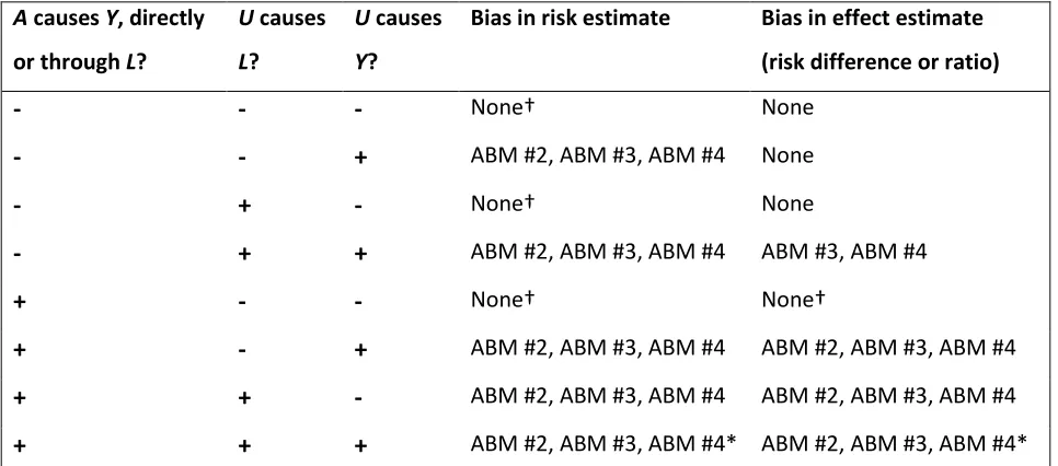
[image:41.612.66.549.346.559.2]U differs between populations. Table 1.4 presents a summary of the potential for bias in ABMs.
Table 1.4: Summary of potential for non-transportability and collider bias in risk and causal effect estimates obtained by ABMs, when only the distribution of U differs between populations.
A causes Y, directly or through L?
U causes
L?
U causes
Y?
Bias in risk estimate Bias in effect estimate (risk difference or ratio)
-
-
-
None† None-
-
+
ABM #2, ABM #3, ABM #4 None-
+
-
None† None-
+
+
ABM #2, ABM #3, ABM #4 ABM #3, ABM #4+
-
-
None† None†+
-
+
ABM #2, ABM #3, ABM #4 ABM #2, ABM #3, ABM #4+
+
-
ABM #2, ABM #3, ABM #4 ABM #2, ABM #3, ABM #4+
+
+
ABM #2, ABM #3, ABM #4* ABM #2, ABM #3, ABM #4*†When U is not a cause of either L or Y, and when the only difference between populations is in the (marginal) distribution of U, then there will be no bias in the risk or effect estimates. However, if the populations differ in the distribution of A or in other causes of Y, then there may be bias.
28 Scenario 1: True treatment effect is null in all populations
Consider the DAG in Figure 1.4. Treatment (A) affects CD4 cell count (L). However, neither treatment nor CD4 cell count has any effect on mortality (Y). The table provides examples for two populations of 10000 individuals whose covariate distributions are described by the DAG above, and
which only differ in the prevalence of U=1 (45% in the base-case and 15% in the low-risk population). Without knowledge of U, the g-formula for the low-risk population in Figure 1.4 can be estimated using equation 1, and correctly estimates the null effect and the probability of death in this population under
each treatment value (21.0%).
𝑓𝑓[𝑌𝑌|𝐴𝐴=𝑎𝑎] =� 𝑓𝑓[𝑌𝑌|𝐿𝐿,𝐴𝐴=𝑎𝑎]𝑓𝑓[𝐿𝐿|𝐴𝐴=𝑎𝑎]
𝐿𝐿
[image:42.612.72.532.279.522.2](1)
Figure 1.4: Causal graph depicting a single time point with treatment A, outcome Y, covariate L, and an unknown variable U. The true causal effect of treatment on the outcome is null, and U is a cause of L and Y. The tables provide possible data for 10,000 individuals in two populations: base case and low risk.
29
account for the presence of U, and will still return the correct probability of mortality in the low-risk population for each treatment value (𝑓𝑓[𝑌𝑌]) and risk difference.
𝑓𝑓[𝑌𝑌|𝐴𝐴=𝑎𝑎] =
=� � 𝑓𝑓[𝑌𝑌|𝑈𝑈,𝐿𝐿,𝐴𝐴=𝑎𝑎]
𝑈𝑈
𝑓𝑓[𝐿𝐿|𝑈𝑈,𝐴𝐴=𝑎𝑎]𝑓𝑓[𝑈𝑈]
𝐿𝐿
= � 𝑓𝑓[𝑌𝑌|𝑈𝑈]𝑓𝑓[𝑈𝑈]
𝑈𝑈
� 𝑓𝑓[𝐿𝐿|𝑈𝑈,𝐴𝐴=𝑎𝑎]
𝐿𝐿
=𝑓𝑓[𝑌𝑌]
(2)
Thus, the estimates from the parametric g-formula in a single dataset are expected to produce
unbiased estimates of the risk of the outcome and of the causal effect of treatment on the outcome for
that dataset despite the exclusion of information on U from the models, assuming the identifiability assumptions for causal inference hold – namely, conditional exchangeability of the treated and
untreated given patient histories (no unmeasured common causes of treatment and the outcome),
positivity for treatment strategies, consistency of treatment definition, and no misspecification of the
models for the conditional probability distributions of the confounder and the outcome.
Now, let 𝑓𝑓1represent a function estimated in the base case population and let 𝑓𝑓2 represent a
function estimated in the low-risk population. Using this new notation, the model suggested by ABM #1,
where all input probabilities are estimated in the cohort of interest, can be written as in equation 3.
Regardless of whether we have information on U, ABM #1 gives us unbiased estimates of both the risk and the causal effect in the cohort of interest, under the same identifiability assumptions as the
g-formula.
𝑓𝑓2[𝑌𝑌|𝐴𝐴 =𝑎𝑎] =� 𝑓𝑓2[𝑌𝑌|𝐿𝐿,𝐴𝐴=𝑎𝑎]𝑓𝑓2[𝐿𝐿|𝐴𝐴=𝑎𝑎] 𝐿𝐿
30
In ABM #2 all input probabilities are estimated from the base-case cohort (as shown by the
index f1), rather than the population of interest (equation 4). Unless all distributions are the same in both populations, equation 4 will be biased.
𝑓𝑓2[𝑌𝑌|𝐴𝐴 =𝑎𝑎]≠ � 𝑓𝑓1[𝑌𝑌|𝐿𝐿,𝐴𝐴 =𝑎𝑎]𝑓𝑓1[𝐿𝐿|𝐴𝐴=𝑎𝑎] 𝐿𝐿
=𝑓𝑓1[𝑌𝑌] (4)
For the example in Figure 1.4, the ABM #2 estimate of the mortality risk in the treated and
untreated in the low-risk population is 33%, not 21%. This is the risk in the base-case population, but is
incorrect for the low-risk population. The difference in the distribution of U between the two populations created a lack of transportability in the risk estimates. However, since the null is true in
both populations, the causal effect estimate obtained from ABM #2 will be correct.
Now consider ABM #3, where the input probabilities are selected from both the cohort of
interest and the base-case cohort. Here, the probability of death Y given treatment A is estimated from the base-case and is used to estimate the risk in the other cohort. Thus, the distribution of Y used for the ABM should be denoted with 𝑓𝑓1, but the distribution of L used in this ABM comes from the cohort of interest and is denoted with 𝑓𝑓2, as in equation (5).
𝑓𝑓2[𝑌𝑌|𝐴𝐴 =𝑎𝑎]≠ � 𝑓𝑓1[𝑌𝑌|𝐿𝐿,𝐴𝐴 =𝑎𝑎]𝑓𝑓2[𝐿𝐿|𝐴𝐴=𝑎𝑎] 𝐿𝐿
(5)
It is clear that unless 𝑓𝑓1[𝑌𝑌|𝐿𝐿,𝐴𝐴 =𝑎𝑎] =𝑓𝑓2[𝑌𝑌|𝐿𝐿,𝐴𝐴=𝑎𝑎], the risk estimate will be biased. In
addition, we can no longer expect the causal effect estimate to be unbiased, even when the null is true
in both populations. In the Figure 1.4 example, the risk difference estimate using ABM #3 is 2.5