White Rose Research Online URL for this paper:
http://eprints.whiterose.ac.uk/89488/
Version: Published Version
Conference or Workshop Item:
Hodge, Victoria Jane orcid.org/0000-0002-2469-0224, Krishnan, Rajesh, Jackson, Tom et
al. (2 more authors) (2011) Short-Term Traffic Prediction Using a Binary Neural Network.
In: 43rd Annual UTSG Conference, 05-07 Jan 2011, Open University.
[email protected] https://eprints.whiterose.ac.uk/ Reuse
Items deposited in White Rose Research Online are protected by copyright, with all rights reserved unless indicated otherwise. They may be downloaded and/or printed for private study, or other acts as permitted by national copyright laws. The publisher or other rights holders may allow further reproduction and re-use of the full text version. This is indicated by the licence information on the White Rose Research Online record for the item.
Takedown
If you consider content in White Rose Research Online to be in breach of UK law, please notify us by
SHORT-TERM TRAFFIC PREDICTION USING A BINARY
NEURAL NETWORK
Dr Victoria Hodge Dr Rajesh Krishnan Dr Tom Jackson Research Associate Research Associate Project Co-ordinator University of York Imperial College London University of York
Prof. Jim Austin Prof. John Polak Professor Professor
University of York Imperial College London
Abstract
This paper presents a binary neural network algorithm for short-term traffic flow prediction. The algorithm can process both univariate and multivariate data from a single traffic sensor using time series prediction (temporal lags) and can combine information from multiple traffic sensors with time series prediction ( spatial-temporal lags). The algorithm provides Intelligent Decision Support (IDS) for road network managers to proactively manage problems on the network as the predictions generated may be used to determine if traffic control interventions need to be applied. The algorithm can operate in near-real-time and dynamically; using data from UTC or UTMC systems. It is based on the Advanced Uncertain Reasoning Architecture (AURA) k-nearest neighbour prediction algorithm, which is designed for scalability and fast performance. The AURA k-NN predictor outperforms other machine learning techniques with respect to prediction accuracy and is able to train and predict rapidly. The basic AURA k-NN time series prediction algorithm was extended by incorporating average daily profiles and variable weighting into the prediction in this paper. The average daily profile of a variable is calculated as the average reading of the variable for a particular time of day and day of the week after removing outliers. When data vectors are matched in the AURA k-NN, the daily profile adds an extra dimension to the match. This process was further enhanced by weighting the profile using variable weighting to vary the profile’s significance. It is shown that incorporating these two additional aspects improves the accuracy of the prediction compared to the standard AURA k-NN, resulting in a very fast and accurate traffic prediction tool
Introduction
Road network management in the UK involves manual traffic monitoring and intervention implementation to supplement timetabled or automated traffic control systems. For example, the UK motorway network is monitored and controlled by the National Traffic Control Centre (Highways Agency 2009) and the road network in counties and cities is monitored and controlled by the traffic control centres run by respective authorities, e.g. London Traffic Control Centre (Barton 2004). The network operators pinpoint traffic problems, determine the likely cause of a problem and then select the most appropriate intervention to both manage the traffic network and mitigate the congestion. Such intervention measures are often based on the operational experience of the person handling the problem.
The remainder of the paper: provides a concise review of traffic prediction methods, presents the proposed binary neural network predictor, provides an evaluation of the predictor with and without the enhancements proposed, the results of this evaluation are analysed and conclusions are provided.
Short-term Traffic Prediction
The objective of the work in this paper was to predict future traffic variable values over short term intervals. The predicted value may then be either displayed to the traffic operator to allow them to visualise how the predicted value will develop over the near future or to select the best course of action. Traffic monitoring systems generate
a
large amount of near-real-time and historic traffic data from various sensors and systems at any given Local Authority (LA) at frequent intervals. Traditional data management technologies such as relational databases would be too slow for an on-line IDS that requires near real-time processing to generate the predictions between data collections. Also, the traffic data are often non-stationary so any predictor needs to be able to process non-stationary data while still maintaining fast, flexible processing. Lastly, the predictor should be able to provide accurate multi-step ahead predictions.Short-term prediction algorithms can broadly be classified into univariate and multivariate approaches. Simple univariate prediction models predict the future value of a single variable as a function of the same variable observed in the (immediate) past. Ding et al. (2002) used support vector machines (Vapnik, 1995) to model future traffic flows. The ARIMA methodology (Box and Jenkins, 1976) is a popular statistical technique for time series prediction. Hamed and Al-Masaeid (1995) used an ARIMA(0,1,1) model to predict 1 minute ahead traffic flows. Williams and Hoel (2003) added seasonal differencing to their ARIMA model to predict flows using a seasonal periodicity of 1 week. More recently, Ghosh et al. (2007) used a seasonal ARIMA model calibrated using Bayesian methods to predict traffic flows. However, ARIMA has high computational complexity and requires time consuming optimisation and conventional ARIMA assumes that the data series is stationary. Detailed statistical knowledge is required to determine the order of the ARIMA model that provides the most accurate prediction, and this is usually done manually. Automating this process will require time consuming optimisation which makes it unsuitable for online applications, since the optimal model specification may vary based on traffic conditions (e.g. presence of incidents).
In contrast to the univariate techniques, a multivariate approach can use data from several traffic sensor locations to generate the prediction as well as multiple traffic variables from a single sensor, potentially providing more accurate prediction results. Kamarianakis and Prastacos (2003) introduced a spatio-temporal extension of ARIMA to predict future traffic flows as a function of historical flows from a given sensor location and its upstream neighbours, which has the drawback of ARIMA models described above.
Various neural networks are used in the literature for multivariate traffic prediction. However, many neural networks require intensive tuning to ensure optimal performance. In an IDS system, the neural network would have to be retrained, probably daily to maintain an up-to-date model, which introduces high computational complexity. For example, Vlahogianni et al. (2005) demonstrated a genetic algorithm for optimising the parameters of Multi-Layer Perceptrons (MLPs). This limits the application of neural networks for online IDS applications.
The k-NN approach satisfies all the requirements for an online predictor for IDS. K-NN can naturally incorporate spatially and temporally lagged variables. The method does not require frequent re-calibration. However, the k-NN method when implemented using traditional relational database management technologies, is computationally slow for large datasets. The neural network-based k-NN predictor, AURA k-NN, is computationally efficient and is able to overcome this problem; the method is up to four times faster than the standard k-NN (Hodge et al., 2005). The AURA k-NN can predict future traffic flows by matching time series against a set of historical time series and using the matches to extrapolate and predict; the methodology satisfies the five criteria above (Hodge et al., 2010b). The AURA k-NN can process a broad spectrum of traffic data variables such as data from vehicle counts, vehicle speeds, bus timetable adherence, congestion metrics, roadworks data, events data and weather data. This paper further develops the AURA k-NN to improve prediction accuracy by incorporating average daily profiles into the data vectors and variable weighting for the profile variables.
Binary Neural Network for prediction
The objective for the predictor algorithm is to accurately predict the future traffic variable values to allow an operator to visualise how the traffic state will develop or to select the best course of action. Conceptually, the AURA k-NN identifies a set of historical time periods when the set of traffic observations on the road network were most similar to the current set of observations. The method then uses these matches to extrapolate and produce a prediction of the future traffic value by averaging the variable value across the set of matches. The AURA k-NN for prediction is described next.
AURA k-NN
AURA is a library of methods based upon binary neural networks. It is designed for high speed search and matching operations in large data sets and is fast, scalable and compact. The foundation of AURA is the binary Correlation Matrix Memory (CMM), a binary matrix used to store and retrieve patterns (Austin et al., 1998). In the AURA k-NN (Hodge and Austin, 2005; Hodge et al., 2010a; Krishnan et al., 2010a; Krishnan et al., 2010b), each column of the CMM is a set of variable observations (pattern) and each row indexes a variable value or a quantised range of values. This approach was extended to match time series vectors and then to generate multivariate predictions (Hodge et al., 2010b). The AURA k-NN is developed further here by incorporating an additional variable, the average daily profile and by weighting the profile to vary the profile’s influence on the overall match to improve prediction accuracy.
Time Series
For time series prediction, the system must incorporate a time component. A description of how the AURA k-NN accommodates temporal data aspects is given next.
Given the current set of traffic variable values as a vector Xn, and a dataset of past vectors
{X}, k-NN identifies the k nearest neighbours of Xn in {X} using a distance metric. The data
vectors are time-series representations of both sensor readings and sensor average daily profiles: both single sensors (univariate data) and spatially-distributed sets of sensors. To produce the time series, the AURA k-NN predictor effectively buffers the historical sensor data and average daily profiles and accumulates data for a preset time interval PT. Buffering always preserves the temporal ordering of the data. Thus, Buffer = {Buffert: t ε PT}. Then the
time-series for Xn, which we call XnTS, is as given in equation 1:
XnTS = {x1t-3, x1t-2, x1t-1, x1t, x2t-3, x2t-2,…,xnt-3, xnt-2, xnt-1, xnt} (1)
for PT of four time slices {t-3, t-2, t-1, t}. The number of time slices, or temporal lags,will vary as appropriate.
For example, for two 2 variable sensors where sensor1 has readings of 41, 62, 55, 68 for
variable1 and readings of 15.0, 31.0, 25.0, 45.0 for variable2 for four time slices {t-3, t-2, t-1,
t} respectively and sensor2 has readings of 38, 38, 66, 68 and readings of 14.0, 14.0, 35.0,
Xn TS
= {41, 62, 55, 68, | 15.0, 31.0, 25.0, 45.0, | 38, 38, 66, 68, | 14.0, 13.0, 35.0, 45.0} (2)
where the vertical bars illustrate the sections of the pattern with each section representing the time series for one variable.
Learning in the AURA k-NN
CMMs learn associations between input patterns and output patterns. The input pattern (In)
represents the set of all variable values for a particular set of observations and indexes CMM matrix rows. The output pattern (On) indexes the matrix columns and uniquely identifies that
record. There is one input-output association for each record n in the data set of N records.
CMMs learn binary patterns as the matrices are optimised for compactness and speed so numeric variables must be quantised (binned) to allow mapping to a binary pattern (Hodge and Austin, 2005). In AURA, quantisation maps observations of a continuous variable into a set of discrete values or bins. Each variable is quantised over its entire range of values to a set of bins where each bin indexes a specific and unique row in the CMM. For example, for an integer-valued variable with range 0-99 and 5 bins then each bin would have width 20: bin0
holds the variable values {0..19} and would index CMM row 0, bin1 stores {20..39} …bin4
holds {80..99} and would index CMM row 4. For a real-valued variable with range [0.0-100.0] and 5 bins then each bin would have width 20. Thus, for sensor1 and sensor2 above, the set
of bin mappings (bin indices for each variable value) for XnTS are given in equation 3:
Bins(XnTS) = {2, 3, 2, 3, | 0, 0, 1, 2, | 1, 1, 3, 3, | 0, 0, 1, 2} (3)
To produce the input pattern In,each bin index in equation 3 maps to a binary representation.
For a variable with five bins, the five binary representations are then bin0 = 00001, bin1 =
00010, bin2 = 00100 etc. Thus, the bins corresponding to the values in XnTS in historic data
record {XTS} are marked 1 while the other bins are marked 0 in In. The binary representations
for all the variables and their respective time slices in the original data vector are concatenated to create the binary pattern In as given in equation 4 which is the binary
representation of the bin mappings in equation 3. The binary representation is a learning pattern to be stored in the CMM to allow the particular data to be stored and retrieved.
In = {00100 01000 00100 01000 | 00001 00001 00010 00100 | 00010 … } (4)
The storage structure consisting of binary patterns, as in equation 4, for all N observations in the data set {XTS} is called a Correlation Matrix Memory (CMM). Training the CMM is a one-pass process with one training step for each binary input pattern in the data set so training is rapid. Each binary pattern In is associated with a unique identifier pattern On which has a
single bit set to index a unique column in the CMM as given in equation 5. This column thus indexes the binary pattern In.
OR logical is
where
n
all
∨
∨
×= In OnT
CMM (5)
Retrieving the best matches using the AURA k-NN
For k-nearest neighbour prediction, the CMM is searched to find the k best matches to be used for generating the prediction. The retrieval pattern R is created for each new query XqTS,
using a set of parabolic kernels, with one kernel for each time slice (t ε PT) within each
variable x in XqTS. The kernels emulate Euclidean distance (Hodge and Austin, 2005). For
each time slice for a particular variable, the kernels are identical but they may vary across variables according to the number of quantisation bins assigned to that variable. In this paper, all variables use an equal number of bins and, hence, an equivalent kernel. To implement variable weighting during retrieval, the height of a particular variable’s kernel is varied using a weighting factor ωx. This is applied uniformly across all time slices for that variable. For
example, a weight of 2 doubles the height of the kernels so all time slices for that variable are then assigned weight 2. The kernel density is estimated using equation 6 for all time slices t ε
(
)
(
)
where 2 2 2 2 )) ( ( ) max( ) ( ) ( ) ( ) ( 2 ) max( ) ( nt nt nt h nt q nt x nt x b b x x x bin x bin b x Kernel = − − •=ω α α
(6)
Where, max(b) is the maximum number of bins for any variable, |bin(xntq) – bin(xnth)| is the
number of bins separating the bin mapped to by the variable value for this time slice for the query pattern (xnt
q
) from the bin mapped to by the variable value for this time slice for the stored historical pattern (xnt
h
), and b(xnt) is the total number of bins for variable xn and time
[image:6.612.199.450.188.347.2]slice t.
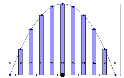
Figure 1. Showing the kernel generated from equation 6 to approximate Euclidean Distance for a variable using 11 quantisation bins and weight 1.
During retrieval, the kernels for all variables are concatenated with each kernel centred on the bin representing the variable value for the query record so that bin receives the highest score from the kernel. Thus the best matching historical records (CMM columns) will receive the highest scores. Using the example above, for an integer-valued variable with range 0-99 and 5 bins then each bin would have width 20: bin0 {0..19}, bin1 {20..39} …bin4 {80..99}. Thus, if
the query value was 31, this would map to bin1 so the input pattern element representing bin1
(indexing from 0) would be the centre of the kernel. Thus, the highest value for this kernel (analogous to the dotted value of the kernel in Figure 1) would be centred on bin1.
This kernel concatenation emulates the scoring of Euclidean Distance. Thus the pattern input to the CMM to retrieve the top k matches is iteratively given by equation 7:
(
Kernel)
forallattributesx offsetR
R'= ⊕ x , (7)
where offset() indexes variable x’s section of the input pattern R and ensures that the kernel is applied to R, centred on the query value for variable x. Thus, each variable indexes a defined set of elements in R.
Figure 2. Illustrating the application of kernels to CMM to find the k-nearest neighbours using time-series vectors with all weighting factors set to 1.
To retrieve the k best matching records, the columns of the matrix are summed according to the value on the rows indexed by the query input pattern R and the CMM produces a summed output vector S as given in equation 8.
∑
•= R CMM
ST (8)
The summed output vector is then thresholded using L-Max thresholding to produce a binary thresholded vector T. L-Max thresholding is used in the AURA k-NN as it retrieves the top L
matching columns. T effectively lists the top L matching columns thus identifying the top k
(where k=L) matches, i.e. the k nearest neighbour data records. An illustration of this process is shown in Figure 2.
Prediction using the AURA k-NN
The basic AURA k-NN time series prediction algorithm is extended by incorporating average daily profiles and variable weighting into the prediction. The average daily profile of a variable is the average reading of the variable for a particular time of day and day of the week after removing outliers. Gibbens and Saacti (2006) discovered that using only this historical average for prediction performed poorly compared to using a k-NN predictor. However, we incorporated the historical average of the sensor to be predicted into the k-NN prediction. The daily profile adds an extra dimension to the match so in equation 1, XnTS
enhanced by weighting the profile using variable weighting, as described in equation 6, to vary the profile’s significance during matching.
For the prediction task in this paper using data arriving at 15 minute intervals, the AURA k-NN retrieves the k top matches and then identifies the t+1 (+15 minute) or t+4 (+1 hour) sensor values for each of the k matches. The t+1 (+15 minute) prediction is then the mean value of the set of t+1 values from the k nearest neighbours and the t+4 (+1 hour) prediction is the mean of the t+4 values. For the 5 minute data, we use t+1 (+5 minutes) and t+12 (+1 hour).
Evaluation
To evaluate the prediction error, various configurations of the AURA k-NN predictor are assessed against each other using the metric in equation 9. The best performing AURA k-NN configurations for data sets 1 and 2 were determined previously (see Hodge et al., 2010b). Therefore, these configurations were used here.
Root Mean Squared Error (RMSE) =
(
)
n F X
n
i
i i
∑
=
−
1
2
(9)
[image:8.612.133.519.382.558.2]The configurations were tested using three data sets, two SCOOT data sets from central London and one UTMC data set from a radial route in York, UK. For each data set, the data is split into train and test sets and the accuracy of the prediction is determined by comparing the predicted and actual flows for the test set. In each separate evaluation, all algorithms used identical data sets. For data sets 1 and 2 erroneous sensor readings were removed using a simple rule: Univariate Screening given in Krishnan (2008). If a historical record contained an erroneous sensor value then the entire record was removed. This was not applied to data set 3 where 0 is a valid flow.
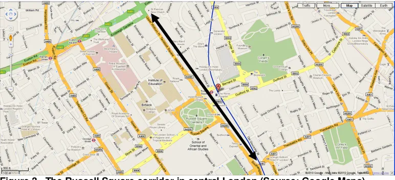
Figure 3. The Russell Square corridor in central London (Source: Google Maps).
Figure 4. Marylebone Road in central London (Source: Google Maps).
Data Set 2. Data set 2 comprised SCOOT ILD data from the ASTRID system for six sensors on the eastbound Marylebone Road in central London as shown in Figure 4. These data contained 15-minute flow values with data range 0-1600. The future flow values at the downstream (easternmost) sensor were predicted. The training data were from May 2008 and 01/06/2008-13/06/2008 while test data were from 16/06/2008-20/06/2008 (one week). Only the weekday data were used giving 2,976 training records and 480 query records. A severe traffic incident happened in Marylebone Rd on 20/06 from 18:59 to 21:01. Therefore, the AURA k-NN may be compared using two analyses, one using all of the testing data from 16/06-20/06 and a second analysis using just data from the incident day, 20/06, which comprised 96 records. The latter analysis provided an indication of how well the configurations performed on incident data when the traffic flow will be anomalous and predictions are potentially more useful to the end-users.
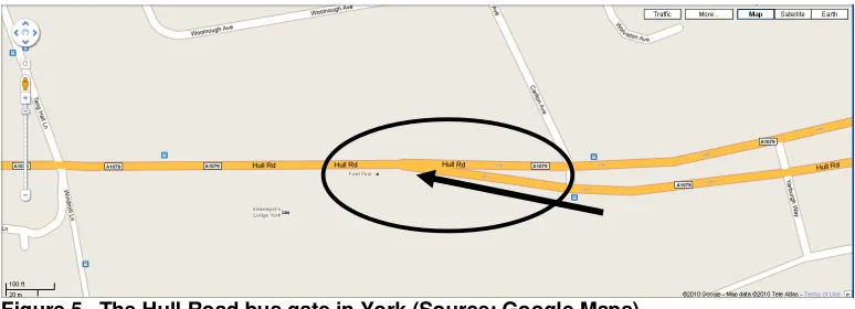
Figure 5. The Hull Road bus gate in York (Source: Google Maps).
[image:9.612.92.479.406.546.2]Evaluation Description
For data set 1, k was set to 50, there were 49 bins per variable and the time series length was 8 (Hodge et al., 2010b). The Russell_FO configuration used the flow and occupancy variables and the sensor whose value was to be predicted was excluded. Russell_F used the flow variable only and the predicted sensor was included. The Russell_F data set had 7 variables so the average daily profile weighting was set to seven or less for data set 1 (i.e. the weight of the profile is equivalent to the combined weight of the variables or less).
For data set 2, k was set to 10, there were 25 bins across all variables and the time series length was 8 (Hodge et al., 2010b). Both the Marylebone and Incident AURA k-NN configurations used all of the flow variables available. Marylebone had 6 variables so the average daily profile was weighted up to six for data set 2 (again, the weight of the profile is equivalent to the combined weight of the variables or less).
For data set 3, k was set to 50, there were 25 bins across all variables and the time series length was 12. The BusGate AURA k-NN configuration had only one variable so only a profile weighting of 1 was tested.
This effectively ran ten tests for each AURA k-NN configuration to identify the overall best performing predictor configuration of those analysed. For each data set configuration, the accuracy of prediction 15 minutes ahead and 1 hour ahead were analysed and there were five data configurations. Two configurations of data set 1 using just flow (Russell_F) and combining flow and occupancy data from the sensors (Russell_FO), data set 2 using the whole test set (Marylebone) and then using just the data from the day of the incident as the test set (Incident) and, finally, one evaluation using data set 3 (BusGate). The characteristics of these data varied and should provide a thorough evaluation of the predictors.
Results
In the following, NoProfile indicates the AURA k-NN with no average daily profile. All other AURA k-NN configurations use the average daily profile. In P1 the average daily profile used weight (ωx) of 1; P2 used weight of 2, and so on. Table 1 lists the RMSE achieved for the
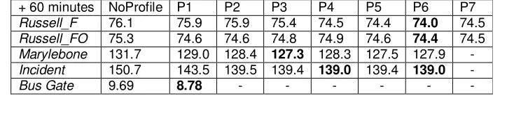
four AURA k-NN configurations when predicting 15 minutes ahead and lists 5 minute ahead prediction for the BusGate data and Table 2 lists the RMSE achieved for all five configurations when predicting 1 hour ahead
Table 1. Listing the RMSE for the various AURA k-NN configurations evaluated for 15 minute prediction on the four data sets and 5 minute prediction of the BusGate data. The best performing profile weight for each configuration is highlighted in grey.
+ 15 minutes NoProfile P1 P2 P3 P4 P5 P6 P7
Russell_F 65.2 64.6 64.6 64.5 64.4 64.5 64.4 64.6
Russell_FO 65.3 64.9 64.7 64.9 64.6 64.8 65.0 65.0
Marylebone 115.9 116.0 115.5 114.6 114.0 114.3 115.7 -
Incident 128.8 125.9 124.8 126.6 127.4 126.4 128.2 -
[image:10.612.146.518.633.715.2]BusGate 7.37 7.22 - - - -
Table 2. Listing the RMSE for the various AURA k-NN configurations evaluated for 1 hour prediction on the five data sets. The best performing profile weight for each configuration is highlighted in grey.
+ 60 minutes NoProfile P1 P2 P3 P4 P5 P6 P7
Russell_F 76.1 75.9 75.9 75.4 74.5 74.4 74.0 74.5
Russell_FO 75.3 74.6 74.6 74.8 74.9 74.6 74.4 74.5
Marylebone 131.7 129.0 128.4 127.3 128.3 127.5 127.9 -
Incident 150.7 143.5 139.5 139.4 139.0 139.4 139.0 -
In table 1, for 15 minute ahead prediction, profile weights 4 and 6 produced the highest accuracy for the Russell_F configuration while weight 4 produced the best result for
Russell_FO. In table 2, for both configurations, the overall best performing profile weighting with respect to 1 hour ahead prediction used a profile with weight of 6. However, across both 15 minute and 1 hour ahead prediction combined, weight 6 performs best for both configurations. There were twelve variables in Russell_FO so a profile weighting of half the total number of variables performs best. For Russell_F with seven variables, the best profile weight was one fewer than the total number of flow variables.
With no profile, Russell_FO outperformed Russell_F. However, when the profile was incorporated then Russell_F outperformed Russell_FO. This indicates that the occupancy variable used in Russell_FO was not necessary when profiles were used and best results were achieved using only flow variables.
For data set 2, the results are less conclusive. However, considering 15 minute and 1 hour ahead prediction together, weight 5 performs best for Marylebone and weight 2 performs best for Incident closely followed by weight 5. There were six variables in both Marylebone
and Incident so a profile weighting of one fewer than the total number of flow variables performs best for data set 2 overall.
For data set 3, using an average daily profile improved the RMSE compared to not using the average daily profile. Thus the profile weighting was equal to the number of flow variables
Using an average daily profile improved the prediction accuracy for all evaluations. This suggests that, if similar time-series occur when the traffic data is normally similar then the outcome (future traffic value) is likely to be similar. The degree of influence of this extra matching also needs to be carefully considered. The results indicate that the RMSE does not fall and then rise monotonically as the weight increases but is inconsistent. For all evaluations with flow variables only, the weighting of the profile should be one fewer than the total number of flow variables with a minimum value of 1 to gain the greatest prediction accuracy.
Conclusion
Using an average daily profile (historical average) improved the recall accuracy of the AURA k-NN in all evaluations. For multivariate data sets, weighting the profile variable further improved the root mean squared error compared to using an un-weighted profile. When using a weighted profile using only flow variables outperformed using both flow and occupancy for data set 1. For weighting the profile with these data sets, we were able to identify a heuristic that performed well, use a profile weight one fewer than the number of flow variables with a minimum value of 1. This needs to be validated against other datasets.
The AURA k-NN predictor will be incorporated into an IDS system for traffic monitoring and will be tested against real-world data from London, Kent and York in the UK. By using predictions, the IDS will be able to make recommendations proactively and anticipate traffic problems rather than functioning reactively as there may be latency in the data collection.
Acknowledgements
The work reported in this paper forms part of the FREEFLOW project, which is supported by the UK Engineering and Physical Sciences Research Council, the UK Department for Transport and the UK Technology Strategy Board. The project consortium consists of partners including QinetiQ; Mindsheet; ACIS; Kizoom; Trakm8; City of York Council; Kent County Council; Transport for London, Imperial College London and University of York.
References
Barton, N. (2004). Keeping London Moving: Real Time Traffic Management Systems and Operations in Transport for London. Proceedings of the 32nd Annual European Transport Conference (ETC), Strasbourg, France. 4-6 October 2004.
Box, G.E. and Jenkins, G.M. (1976). Time Series Analysis: Forecasting and Control. Holden-Day, San Francisco.
Ding, A., Zhao, X. and Jiao, L. (2002), Traffic Flow Time Series Prediction Based On Statistics Learning Theory. In, Procs IEEE 5th International Conference on Intelligent Transportation Systems, pp. 727-730.
Ghosh, B., Basu, B. and O'Mahony, M. (2007), Bayesian time-series model for short-term traffic flow forecasting, Journal of Transportation Engineering (ASCE) 133(3): 180-189.
Gibbens, R.J. and Saacti, Y. (2006). Road traffic analysis using MIDAS data: journey time prediction University of Cambridge, UCAM-CL-TR-676, ISSN 1476-2986
Glover, P., Rooke, A. and Graham, A. (2008). Flow diagram, Thinking Highways, 3(3):20-23.
Gorry, G.A. and Scott-Morton, M.S. (1971). A framework for management information systems, Sloan Management Review, 13(1):55-70.
Hamed, M. M. and Al-Masaeid, H. R. (1995), Short-term prediction of traffic volume in urban arterials, Journal of Transportation Engineering (ASCE) 121(3): 249-254.
Highways Agency, 2009. National Traffic Control Centre. Available from http://www.highways.gov.uk/knowledge/1298.aspx. Accessed on 25 Oct. 2010.
Hodge, V.J. and Austin, J. (2005). A Binary Neural k-Nearest Neighbour Technique. Knowledge and Information Systems, 8(3): 276–292, Springer-Verlag London Ltd.
Hodge, V.J., Krishnan, R., Austin, J., and Polak, J. (2010a). A computationally efficient method for online identification of traffic incidents and network equipment failures. Transport Science and Technology Congress: TRANSTEC 2010, New Delhi, India, April 4-7 2010.
Hodge, V.J., Krishnan, R., Jackson, T., Austin, J., and Polak, J. (2010b). Short-Term Traffic Prediction Using a Binary Neural Network. Submitted to, Neural Networks, Elsevier, 2010.
Hunt, P. B.; Robertson, D. I.; Bretherton, R. D. & Winton, R. I. (1981), SCOOT - a traffic responsive method of coordinating signals Transport and Road Research Laboratory, Crowthorne, Berkshire, UK. 1981.
Kamarianakis, Y. and Prastacos, P. (2003), Forecasting traffic flow conditions in an urban network: Comparison of multivariate and univariate approaches, Transportation Research Record: Journal of the Transportation Research Board, 1857: 74-84.
Kindzerske M.D and Ni, D. (2007). A Composite Nearest Neighbor Nonparametric Regression to Improve Traffic Prediction. Transportation Research Record: Journal of the Transportation Research Board, 1993: 30-35.
Krishnan, R., (2008). Travel time estimation and forecasting on urban roads, PhD thesis, Imperial College London.
Krishnan, R. and Polak, J.W. (2008). Short-term travel time prediction: An overview of methods and recurring themes, Proceedings of the Transportation Planning and Implementation Methodologies for Developing Countries Conference (TPMDC 2008), Mumbai, India, December 3-6, 2008. CD-ROM
Krishnan, R., Hodge, V.J., Austin, J., Polak, J. and Lee, T-C. (2010b). On Identifying Spatial Traffic Patterns using Advanced Pattern Matching Techniques. In, Transportation Research Board (TRB) 89th Annual Meeting, Washington, D.C., January 10-14, 2010. (DVD-ROM: 2010 TRB 89th Annual Meeting: Compendium of Papers)
Turban, E. and Aronson, J. 1997. Decision Support Systems and Intelligent Systems. 5th. Prentice Hall PTR. ISBN:0137409370
Vapnik, V. (1995). The nature of statistical learning theory. New York: Springer-Verlag, ISBN: 0387987800.
Vlahogianni, E.I., Karlaftis, M.G. and Golias, J.C. (2005). Optimized and meta-optimized neural networks for short-term traffic flow prediction: A genetic approach, Transportation Research Part C: Emerging Technologies, 13(3): 211-234, ISSN 0968-090X.