Transparent boundary conditions based on the pole condition for time-dependent, two-dimensional problems.

for time-dependent, two-dimensional problems.

.

White Rose Research Online URL for this paper:

http://eprints.whiterose.ac.uk/90545/

Version: Accepted Version

Article:

Ruprecht, D, Schädle, A and Schmidt, F (2013) Transparent boundary conditions based on

the pole condition for time-dependent, two-dimensional problems. Numerical Methods for

Partial Differential Equations, 29 (4). 1367 - 1390. ISSN 0749-159X

https://doi.org/10.1002/num.21759

[email protected] https://eprints.whiterose.ac.uk/ Reuse

Unless indicated otherwise, fulltext items are protected by copyright with all rights reserved. The copyright exception in section 29 of the Copyright, Designs and Patents Act 1988 allows the making of a single copy solely for the purpose of non-commercial research or private study within the limits of fair dealing. The publisher or other rights-holder may allow further reproduction and re-use of this version - refer to the White Rose Research Online record for this item. Where records identify the publisher as the copyright holder, users can verify any specific terms of use on the publisher’s website.

Takedown

If you consider content in White Rose Research Online to be in breach of UK law, please notify us by

PROBLEMS

DANIEL RUPRECHT∗_{, ACHIM SCH ¨ADLE}†_{, AND FRANK SCHMIDT}‡

Abstract. The pole condition approach for deriving transparent boundary conditions is ex-tended to the time-dependent, two-dimensional case. Non-physical modes of the solution are iden-tified by the position of poles of the solution’s spatial Laplace transform in the complex plane. By requiring the Laplace transform to be analytic on some problem dependent complex half-plane, these modes can be suppressed. The resulting algorithm computes a finite number of coefficients of a series expansion of the Laplace transform, thereby providing an approximation to the exact boundary condition. The resulting error decays super-algebraically with the number of coefficients, so relatively few additional degrees of freedom are sufficient to reduce the error to the level of the discretization error in the interior of the computational domain. The approach shows good results for the Schr¨odinger and the drift-diffusion equation but, in contrast to the one-dimensional case, exhibits instabilities for the wave and Klein-Gordon equation. Numerical examples are shown that demonstrate the good performance in the former and the instabilities in the latter case.

Key words. transparent boundary condition, non-reflecting boundary condition, pole condition, wave equation, Klein Gordon equation, Schr¨odinger equation, drift diffusion equation

1. Introduction. Transparent boundary conditions (TBCs) are required when-ever a problem is posed on a domain that has to be truncated in order to become numerically treatable, either because it is unbounded or too large to compute solu-tions in a reasonable amount of time. Usually, TBCs have to avoid reflecsolu-tions at the artificial boundary, although more complex situations can arise, for example if inho-mogeneities are present in the truncated part. Exact TBCs are typically non-local in time and space and suitable approximations have to be derived in order to be able to efficiently compute numerical solutions to the truncated problem. The study of this type of boundary conditions started in the 1970s, see the paper of E. L. Lindman [15] and references given there. In their seminal paper [5] Engquist and Majda devised a general strategy for the derivation of approximate TBCs. Comprehensive overviews of the subject can be found, for example, in [2, 7, 8, 9, 23].

The pole condition approach for the derivation of TBCs was introduced in a first version in [20, 22] for time-dependent Schr¨odinger-type equations, later in [12, 13, 19] for time-harmonic scattering problems. It was further explored in [6, 11, 16, 21]. An alternative formulation of the pole condition is presented in [17], which provides a noticeably simplified implementation and is also used in the present paper. A com-parison of different techniques to derive TBCs for Schr¨odinger’s equation can be found in [2], finding the pole condition to be one of the most efficient. In [18], the pole condi-tion approach is adopted for a larger class of time-dependent problems, showing good performance for different types of partial differential equations (PDEs) ranging from Schr¨odinger’s equation, the heat equation to wave and Klein-Gordon equation. How-ever, the experiments involved only one-dimensional or two-dimensional wave-guide

∗_{Institute of Computational Science, USI Lugano, CH-6904 Lugano, Switzerland.}

E-mail: [email protected]. Supported by the Swiss HP2C initiative.

†_{Mathematisches Institut, Heinrich-Heine-Universit¨at, D-40255 D¨usseldorf, Germany.}

E-mail: [email protected]

‡_{ZIB Berlin, D-14195 Berlin, Germany.}

E-mail: [email protected]. Supported by the DFG Research CenterMatheon”Mathematics for key technologies” in Berlin.

1

geometries. The present paper extends this approach to the fully two-dimensional case and investigates its performance through numerical experiments. While the very good performance of the pole condition is confirmed in the two-dimensional case for Schr¨odinger’s equation and the drift-diffusion equation, instabilities are found for the wave equation.

As the infinite element method, see [3], the pole condition does not truncate the exterior domain at some finite length. Nevertheless, the finite number of expansion coefficients of the Laplace transform also results in some form of truncation and the pole condition realizes a radiation boundary condition at the boundary of the in-terior domain and does not aim at providing a meaningful solution in the exin-terior. In some special cases, see [25], the pole condition is closely related to the perfectly matched layer approach introduced in [4], but as it does not require complex coordi-nate stretching, the pole condition provides a more general framework. Note that in contrast to other approaches to TBC involving Laplace transforms, for example [1], the pole condition applies the Laplace transform in space and not in time.

The class of problems considered are, as in [18], initial value problems for linear PDEs of the form

p(∂t)u(t,x) =c2∆u(t,x)−d· ∇u(t,x)−k2u(t,x) forx∈R2, t≥0. (1.1)

Included here are the Klein-Gordon equation for p(∂t) = ∂tt and d = (0,0)T, the drift-diffusion equation forp(∂t) =∂tandk= 0, the heat equation forp(∂t) =∂tand d= (0,0)T_{,k= 0 and finally Schr¨odinger’s equation forp(∂}

t) =i∂tandd= (0,0)T,

k= 0. Equation (1.1) is to be solved on a finite computational domain Ω⊂R2_with

some boundary conditionB(u) = 0 on∂Ω, such that on the domain Ω the solution of the initial boundary value problem approximates the solution of the unrestricted initial value problem.

If the support of the initial valueu(0,x) is a subset of Ω and the exterior domain is homogeneous, in the linear case the boundary condition has to suppress all modes traveling from the exteriorR2_{\Ω into the computational domain. Section 2 illustrates}

the main concept of the pole condition by means of a simple one-dimensional example. Section 3 introduces the details of the discretization employed in the two-dimensional case and Section 4 shows several numerical examples.

2. Pole condition. This section provides a brief sketch of the key idea of the pole condition. Denote the Laplace transform of some functionf along some (spatial) coordinaterby

L(f)(s) =

Z ∞

0

exp(−sr)f(r)dr. (2.1)

The pole condition exploits the identity

exp(ar)7→L 1

s−a, (2.2)

RegionC_{in for different equations as derived in [18].}

Equation Parameters in (1.1) C_in

Schr¨odinger equation p(∂t) =i∂t,d= 0, k= 0 {z∈C: Re(z)>−Im(z)} Drift-diffusion equation p(∂t) =∂t,k= 0 {z∈C: Re(z)>0}

Wave equation p(∂t) =∂tt,d= 0, k= 0 {z∈C: Im<0} Klein-Gordon equation p(∂t) =∂tt, d= 0 {z∈C: Im<0}

modes and a half-plane C_{out containing all outgoing modes. Note that these}

half-planes depend on the equation at hand: Table 2.1 quotes the regions corresponding to the equations mentioned above as derived in [18]. For a givenC_{in, the pole}

condi-tion is then defined as follows:

Definition 2.1. Let u(t, r)be a function depending on timet and some spatial coordinate r. Denote its Fourier transform in t by uˆ and the dual variable to t by

ω. Then u satisfies the pole condition, if U(ω, s) := L(ˆu(ω,·))(s) has an analytic extension toC_{in for everyω.}

To illustrate this concept, consider the one-dimensional wave equation on a semi-infinite interval

∂ttu(x, t) =∂xxu(x, t), x∈Ω = [−1,∞) (2.3)

and assume that a boundary condition at x= 0 is sought such that the solution of (2.3) coincides with the solution on the restricted domain [−1,0]. Here, the r from Definition 2.1 is identical to the spatial coordinatex. Inserting an ansatz

u(x, t) = exp(−iωt) exp(ikx) (2.4)

into (2.3) yields the dispersion relation

ω=±k (2.5)

and assumingω >0 without loss of generality yields solutions of the form

u(x, t) =c1exp (−iωt) exp (iωx) +c2exp (−iωt) exp (−iωx), (2.6)

where the first term corresponds to the positive branch of the dispersion relation and is rightward moving while the second term corresponds to the negative branch and is leftward moving. Let the non-physical modes in this example be the modes traveling leftwards from (0,∞) into the interval [−1,0]. The pole condition then has to suppress the pole corresponding to the second term in (2.6).

In order to point out the connection between the two modes in (2.6) and their corresponding poles, we derive an equation for U = L(u) from (2.3). The Laplace transform satisfies the identity

L(∂xxf)(s) =s2L(f)(s)−sf0−f0′, (2.7)

where f0 and f0′ denote the Dirichlet and Neumann data at x= 0. Further, as in

Definition 2.1, denote byU the function obtained by applying touFourier transform in time and Laplace transform in space. Using (2.7), we obtain from (2.3) the equation

−ω2U(ω, s) =s2U(ω, s)−suˆ0(ω)−uˆ′0(ω)

⇒ U(ω, s) =1 2 ˆ

u0−(i/ω)ˆu′0 s−iω +

1 2 ˆ

u0+ (i/ω)ˆu′0

where ˆu0(ω), ˆu′0(ω) are the Fourier transforms of the time-dependent Dirichlet and

Neumann data u0(t), u′0(t) at x = 0. By (2.2), the first term with pole at iω

cor-responds to the physically correct rightward propagating mode with coefficient c1

in (2.6), the second term with pole at −iω to the non-physical leftward traveling mode with coefficient c2. In order to exclude the non-physical mode, one could for

example setC_{in ={z∈}C_{: Im(z)<0}, so that the pole condition requires U to be}

analytic at −iω, thus removing this pole from U and the corresponding mode from the solution. Note that in this simple one-dimensional example, the pole condition can also be enforced by requiring the numerator of the right term in (2.8) to vanish, leading to

iωuˆ0+ ˆu′0= 0 ↔ ∂tu0−u′0= 0, (2.9)

which is the well known transparent boundary condition for the one-dimensional wave equation, see for example [5].

For more complex problems, an explicit decomposition of U like (2.8) is usually not available. However, the Laplace transform can often still be decomposed into incoming and outgoing parts in terms of path integrals in the complex plane, see [18], hence still allowing to define a region C_{in and a pole condition based transparent}

boundary condition. In particular, this is possible for the different types of equations listed in Table 2.1.

3. Discretization. This section presents the employed discretizations. Subsec-tion 3.1 describes the discretizaSubsec-tion of the exterior domain with special semi-infinite elements and how the pole condition is incorporated. The mapping between the exterior elements and the corresponding reference element introduces a generalized distance coordinate, along which the pole condition is enforced. As the exterior el-ements are semi-infinite, integrals arise that have one limit infinite. A mapping is introduced, converting these integrals into proper integrals in the Hardy space on the complex unit-disc. The discretization of the interior uses standard finite elements and is not elaborated further. Subsection 3.2 describes the employed integration schemes, including the choices of the parameter of the mappings.

3.1. Space discretization. The discretization of the exterior domain uses semi-infinite trapezoids as proposed in [24, 25]. The construction of these exterior meshes is discussed in [14]. Possible other choices would be semi-infinite triangles and rectangles as in [17]. In any case the exterior discretization has to be such that there is a uniform distance variable. For the sake of simplicity, we assume that the computational domain Ω is convex, although a generalization to star-shaped domains should be possible.

Fig. 3.1. Employed basic mesh. Elements triangulating the interior domain are marked in dark grey while the trapezoids decomposing the exterior are marked in light grey. Finer meshes are generated by uniform refinements of the triangles and adding additional rays and exterior elements when new nodes on the boundary emerge.

η

2 h

ξ

h 1

4 a

b

3 2

3 4

1

1 0

0 1 ξ

η

g

x₁ x₂

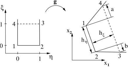
Fig. 3.2. Transformation mapping the reference semi-infinite rectangle to an exterior trape-zoidal element.

drift term is given.

Z

T

∇xu· ∇xv dx=

Z

[0,1]×[0,∞] J−T_∇

ηξu˜·J−T∇ηξv˜|J|d(η, ξ),

Z

T

d· ∇xu v dx=

Z

[0,1]×[0,∞]

d·J−T_∇

ηξu˜ ˜v|J|d(η, ξ).

Z

T

u v dx=

Z

[0,1]×[0,∞]

˜

uv˜|J|d(η, ξ),

(3.1)

The Jacobian of the bilinear mappinggand its determinant are

J =R

hη+ (a+b)ξ −b+ (a+b)η

0 hξ

, |J|=hξ(hη+ (a+b)ξ), (3.2)

whereRis a rotation,hηis the width of the trapezoid,hξis a scaling factor measuring the distance to the boundary and aandb are signed distance variables, compare for Figure 3.2.

term, for example, is given by

Z

[0,1]×[0,∞]

J−T∇ηξu˜·J −T_∇

ηξv˜|J|d(η, ξ) =

Z 1

0

Z ∞

0

∂ηu˜ηu˜ξ ˜

uη∂ξu˜ξ

T

 

h2

ξ+(b−(a+b)η) 2

hη+ξ(a+b)

b−(a+b)η hξ

b−(a+b)η hξ

hη+(a+b)ξ

hξ

 

∂ηv˜η˜vξ ˜

vη∂ξv˜ξ

dξdη.

(3.3)

Functions ˜uη will be approximated using standard finite element basis functions

{φj(η)}, j = 1, . . . , Nη and therefor integrals over the radial coordinate η can be evaluated by quadrature formulas.

3.1.2. Hardy Space. Infinite integrals over the radial coordinateξ are trans-formed to finite integrals in the Hardy spaceH+_(D

0) using the identity

Z ∞

0

˜

f(ξ)˜g(ξ)dξ=−2s0

1 2π

Z

∂D0

(MLf)(¯z)(MLg(z))|dz| (3.4)

whereMdenotes the modified M¨obius transform

H−

(Ps0)→H +_(D

0) : F 7→ MF defined by (MF)(z) :=F

s0 z+ 1

z−1

₁

z−1. (3.5) Here,Ps0 denotes a half-plane in the complex plane, depending on the parameters0,

andD0denotes the complex unit-disc, see Figure 3.3. Further,Mis an isomorphism

between the Hardy spacesH−

(Ps0) andH +_(D

0). Details can be found in [16, 17].

The parameter s0 has to be chosen such that the half-plane Ps0 coincides with

the half-plane C_{in of non-physical poles for the considered problem. As functions in}

the space H−

(Ps0) are analytic on the half-plane Ps0 and M is an isomorphism, a

functionMF is analytic onD0 if and only ifF is analytic onPs0.

Hence the pole condition, stating that the Laplace transformL(f) of some func-tionf has to be analytic onC_{in, is equivalent to the condition thatML(f) is analytic}

onD0for the correct choice of the parameters0. In short, we established the following

sequence of reformulations of the pole condition

f satisfies pole condition :⇔F has analytic extension toC_in

⇔F ∈H−

(Ps0) for correct choice ofs0

⇔ MF ∈H+(D0),

(3.6)

see [16] for details.

In order to derive a formulation, which is easy to implement, some more transfor-mations are required: Given a function f, its image under Land Mis decomposed into

ML(f)(z) = 1 2s0

(f0+ (z−1)F(z)) =:

1 s0 T− f0 F

(z) (3.7)

in order to get a local coupling with the boundary dataf0. As the Laplace transform

maps differentiation to multiplication bys0(z+ 1)/(z−1), straightforward calculation

yields

ML(f′)(z) =1

2(f0+ (z+ 1)F(z)) =:T+

f0 F

0 0 1 i s −s 1 i

Fig. 3.3.Sketch of the M¨obius transformM: H−_(P

s0)→H

+_(D

0), mapping functions defined

on the complex half-planePs0 to functions defined on the complex unit-discD0. The parameters0

has to be chosen such thatPs0 corresponds to theCinsuitable for the problem at hand.

For motivating this coupling, note that it follows from general theory on Laplace transforms that if F is the Laplace transform of f one has lims→∞sF(s) = f(0), wheneverf(0) exists. For details on the decomposition we again refer to [16, 17].

It remains to take care of terms which contain multiplications by ξ and ((a+

b)ξ+hη)−1 in (3.3). To this end, an additional operator P : H+(D0) → H+(D0)

(multiplication byξ)1 _{is implicitly defined by}

ML{(·)f(·)}=M

−(Lf(·))′ =s−1

0 P(MLf).

Direct calculations yield

(PF) (z) =(z−1)

2

2 F

′

(z) +z−1

2 F(z), F∈H

+_(D

0). (3.9)

Assembling the discrete system involves basically the assembly of discrete counterparts of the operatorsT+,T− andP.

3.1.3. Choosing Basis Functions. Up to now, all transformations were on a continuous level and no approximations were made. Because functions that are ana-lytic on the complex unit-disc can be expanded in power series, the set of monomials

zj ∞

j=0 constitutes a basis ofH +_(D

0). By using the space spanned by a finite

num-ber of monomials {zj_}Nξ

j=0 as test and ansatz space, one obtains finite dimensional

approximations ofT±

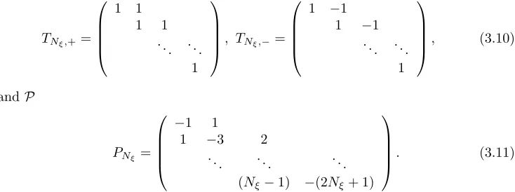
TNξ,+=

     1 1 1 1 . .. ... 1     

, TNξ,− =

    

1 −1 1 −1

. .. ... 1      , (3.10) andP

PNξ =

    

−1 1

1 −3 2

. .. . .. . ..

(Nξ−1) −(2Nξ+ 1)

     . (3.11)

The Hardy space monomials can also be transformed back to give a representation of the corresponding ansatz and test functions in physical space, see [16]. To define the

1

local stiffness matrix, set for theξ-integrals

L(_ξ,−₁₁1):=−2 T⊤

Nξ,− hηs0I+ (a+b)PNξ

−1

TNξ,−,

L(0)_ξ,12:=−2 TN⊤ξ,−TNξ,+, L (0)

ξ,21:=−2 T

⊤

Nξ,+TNξ,−,

L(1)_ξ,22:=−2hηTN⊤ξ,+TNξ,+, L (0)

ξ,22:=−2(a+b)T

⊤

Nξ,+PNξTNξ,+.

(3.12)

Here the superscript counts the leading order ins0 and the subscripts correspond to

the position in the matrix in (3.3). For theη-integrals set

Lη,11:=

Z 1

0 φ′

i(η)

hξ+

((a+b)η−b)2 hξ

φ′ j(η)

Nη

i,j=1,

Lη,12:=

Z 1

0 φ′

i(η)

b−(a+b)η hξ

φj(η)

Nη

i,j=1,

Lη,21:=

Z 1

0 φi(η)

b−(a+b)η hξ

φ′j(η)

Nη

i,j=1,

Lη,22:=

Z 1

0 φi(η)

1

hξ

φj(η)

Nη

i,j=1.

(3.13)

For equations with second order temporal derivatives, the parameter s0 is chosen to

be frequency dependent in Fourier space, to be precises0 =iω, translating back to ∂t in physical space. To avoid the inversion inL(

−1)

ξ,11 in (3.12), additional unknowns

are introduced such that the local stiffness matrices are given by

L(0)_loc=

"

Lη,22⊗L(0)ξ,22+Lη,12⊗L(0)ξ,12+Lη,21⊗L(0)ξ,21 −2Lη,11⊗TN⊤ξ,−

2I⊗TNξ,− −2I⊗(a+b)MNξ

#

L(1)_loc=

"

Lη,22⊗L(1)ξ,22 0

0 −2I⊗hηI

#

. (3.14)

Similarly, local mass matrices corresponding to the mass integral in (3.1) are given by

M_loc(−1):=

"

M_ξ(−1)⊗Mη 0

0 0

#

, M_loc(−2):=

"

M_ξ(−2)⊗Mη 0

0 0

#

(3.15)

where

M_ξ(−1):=−2hξhηTN⊤ξ,−TNξ,−

M_ξ(−2):=−2hξ(a+b)T ⊤

Nξ,−PNξTNξ,−

and Mη:=

Z 1

0

φi(η)φj(η)

Nη

i,j=1. (3.16)

For the drift term set

D_ξ,(0)₁:=−2T⊤

Nξ,−TNξ,+

D_ξ,(−₂1):=−2(a+b)TN⊤ξ,−PNξTNξ,+

D_ξ,(−₃1):=−2T⊤

Nξ,−TNξ,−

and

Dη,1:=hηd˜2

Z 1

0

φi(η)φj(η)

Nη

i,j=1

Dη,2:= ˜d2

Z 1

0

φi(η)φj(η)

Nη

i,j=1

Dη,3:=

Z 1

0

φi(η)( ˜d2(b−(a+b)η) + ˜d1hξ)φ ′ j(η)

Nη

i,j=1

(3.18)

where ( ˜d1,d˜2)T =d˜=Rdis the rotateddvector. The local drift matrices are then

given by

D_loc(0):=

"

D_ξ,(0)₁⊗Dη,1 0

0 0

#

, D_loc(−1):=

"

D(_ξ,−₂1)⊗Dη,2+D(

−1)

ξ,3 ⊗Dη,3 0

0 0

#

(3.19)

In the computational domain Ω standard local finite element matricesM_loc(0),D(0)_locL(0)_loc

without the s0-parameter are obtained. By assembling the local matrices to global

matrices, a spatial semi-discretization of (1.1) is obtained

p(∂t)

M(0)+ 1

s0

M(−1)₊ 1 s2

0

M(−2)_{u(t) =L}(0)_+s 0L(1)

u(t)+

D(0)+ 1

s0

D(−1)_u(t)−k2_M(0)₊ 1 s0

M(−1)₊ 1 s2

0

M(−2)_u(t)

(3.20)

where u(t) is the time-dependent vector of degrees-of-freedom, including the coeffi-cients of the monomial basis functions of the subset ofH+_(D

0) providing the boundary

condition.

3.2. Time discretization. All conducted simulations rely on the method-of-lines approach: The PDE at hand is first discretized in space, as described in sub-section 3.1, leading to the ODE (3.20) for the coefficients. This equation is then integrated in time using different time-stepping schemes indicated below.

3.2.1. Schr¨odinger’s equation. For Schr¨odinger’s equation, (3.20) is solved by the second order accurate, A-stable trapezoidal/mid-point rule. Denoting by un _the approximation tou(nh) att=nhfor some time-step sizeh, the discretization reads

∂tM u(t) =−ic2Lu(t)↔M

un+1_−un

h =−ic

2_Lun+1+un

2 (3.21)

where the mass and stiffness matrix are given byM =M(0)_+s−1 0 M(

−1)_+s−2 0 M(

−2)

andL=L(0)_+s

0L(1). As in the one-dimensional case, non-physical solutions

corre-spond to poles in the first quadrant, hences0is chosen in the third quadrant and set

to

s0=−1−i, (3.22)

3.2.2. Drift-Diffusion equation. In the examples for the drift-diffusion equa-tion, (3.20) is integrated with the A-stable Radau IIA method with three stages of order five, see [10, Sec. IV.5]. The parameters0is chosen to be real and negative, such

that the poles in the positive half-plane are excluded, corresponding to non-physical exponentially increasing solutions. We set

s0=−5, (3.23)

hence poles with positive real part, see Table 2.1, are excluded. The chosen value of

s0 produces good results, but some optimization is probably still possible. However,

the sensitivity of the results to the specific value is rather low, as long as the correct half-plane is excluded.

3.2.3. Wave equation. For the wave equation, poles in the lower complex half-plane have to be excluded, see 2.1. For the wave equation it isp(∂t) =∂tt, correspond-ing top(ω) =−ω2_{in frequency space. As in the one-dimensional case, we choose the}

parameters0 to be frequency dependent, setting

s0=iω. (3.24)

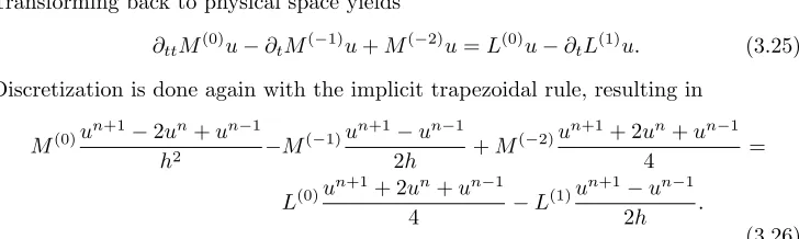
Transforming back to physical space yields

∂ttM(0)u−∂tM(−1)u+M(−2)u=L(0)u−∂tL(1)u. (3.25)

Discretization is done again with the implicit trapezoidal rule, resulting in

M(0)u

n+1_−2un_+un−1

h2 −M

(−1)un+1−un

−1

2h +M

(−2)un+1+ 2un+un

−1

4 =

L(0)un+1+ 2un+un

−1

4 −L

(1)un+1−un

−1

2h .

(3.26)

4. Numerical results. The computational domain in all simulations is a square [−4,4]×[−4,4] in the two-dimensional plane with slightly smoothed corners, see Figure 3.1. Sketched in light gray are the trapezoidal elements spanned by the rays in the exterior domain while the darker triangles correspond to the triangulation of the interior domain. In order to obtain higher resolutions, the shown mesh is refined using up to five uniform refinement steps. As the original mesh is very coarse, no errors are reported for simulations on the unrefined grid, because at least lower order finite elements do not produce reasonable solutions there.

4.1. Schr¨odinger’s equation. For p(∂t) = i∂t, c = k = 0 and d = (0,0)T, equation (1.1) yields Schr¨odinger’s equation. For this case, exact solutions of the form

uα(x, y, t;α) =

i

4t+iexp

−i x2_+y2

−α(x+y)−2α2_t

4t+i

!

(4.1)

with a parameterαare available. We use a superposition of two such solutions, that is

u(x, y, t) =uα(x, y, t;α= 1.4) +uα(x, y, t;α=−2), (4.2)

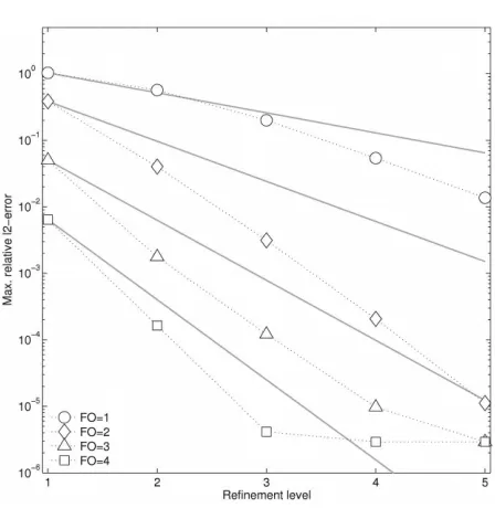
Fig. 4.1. Verification of the spatial order of convergence for the Schr¨odinger equation. Shown is the maximum of the relative l2-errors over all outputs versus the refinement level of the mesh

for finite elements of order one to four. The employed time-step is∆t= 1/6000 and Nξ = 20

coefficients along each ray are used. As a guide to the eye, lines with slopes one to four have been added.

time-step log10(error) Conv. Rate

1/800 -3.8 –

1/1600 -4.4 2.0

1/3200 -5.0 2.0

1/6000 -5.5 2.0

Table 4.1

Maximum relativel2-error over all generated outputs for the Schr¨odinger equation, depending

on the time-step size. The simulation used finite elements of order four, a five times refined mesh andNξ= 20coefficients along each exterior ray.

time-steps ∆t= 1/800,1/1600,1/3200,1/6000 on meshes refined up to five times and for values ofNξ (coefficients per ray) betweenNξ= 1 andNξ = 20. Output is gener-ated at two hundred points in time, distributed equally over the time interval [0,10].

Figure 4.1 shows the maximum relativel2-error over all generated outputs versus

the refinement levels of the mesh for finite elements of order one to four. All elements converge with the expected rate or better until the error saturates at about 3×10−6_in

the case of the higher order finite elements. At this point, the error from the temporal discretization starts dominating, compare for Table 4.1, and increasing the accuracy of the spatial discretization yields no more improvement unless the accuracy of the time-discretization is also increased.

Table 4.1 shows the maximum relativel2-error versus the length of the time-step,

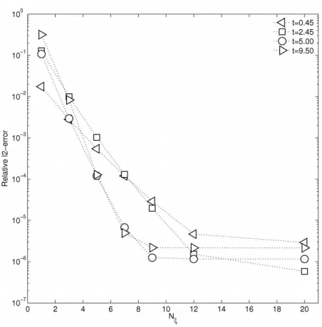
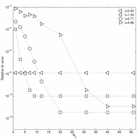
Fig. 4.2. Relativel2-error depending on the number of coefficientsNξ per ray in the exterior

domain for Schr¨odinger’s equation. Maximum error over all generated outputs for finite elements of order one to four on a three times refined mesh.

Figures 4.2 and 4.3 show how the error decays with increasing Nξ. The former shows the maximum relativel2-error for simulations with finite elements of order one

to four, a three times refined mesh and a time-step of ∆ = 1/6000. In all cases, the error decays super-algebraically withNξuntil it saturates at the level of the respective spatial or temporal discretization error. Figure 4.3 shows the error at four different points in time for the fourth order elements. The error decays super-algebraically at all four points in time, even at later times where most of the solution has left the domain.

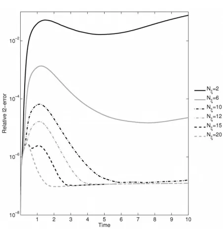
Figure 4.4 shows the relativel2-error over time for different values ofNξ. In all cases, the error increases as the wave packets hit the boundary of the computational domain and subsequently decays to a level determined by the number of coefficients per rayNξ. The error decays faster for larger values ofNξ, but for values ofNξ = 10 or larger, the levels at which the error saturates and in particular the error at the end of the simulation is identical.

4.2. Drift-diffusion equation. Settingp(∂t) =∂tandk= 0 in (1.1) yields the drift-diffusion equation. Note that the heat equation is included here as the special cased= (0,0)T_{. An analytic solution is given by}

u(x, y, t) = 1

texp

− 1

4tc2

h

(x−d1t)2+ (y−d2t)2

i

. (4.3)

Set

d= (d1, d2) = (1.5,1.5), andc= 0.5 (4.4)

and start the integration at t0 = 0.2 with initial value u(x, y, t0). This yields a

Fig. 4.3.Relativel2-error at four fixed points in time depending on the number of coefficients

Nξ per ray for the simulation with finite elements of order four. In all cases, a time-step of ∆ =

1/6000has been used.

time-step log10(error) Conv. Rate

1/10 -3.6 –

1/20 -5.0 4.6

1/30 -5.9 4.9

1/40 -6.5 4.9

1/60 -7.4 4.9

1/80 -8.0 5.0

1/160 -9.2 4.0

Table 4.2

Maximum relativel2-error over all generated outputs depending on the time-step size for finite

elements of order six, a four times refined mesh andNξ= 51coefficients per ray.

advected to the upper right corner of the square while being spread out by diffusion. Integration in time is done by the fifth order Radau IIA(5) scheme. The simulations are run untilT = 5 with finite elements of order one to six, on meshes refined up to four times, values of Nξ between 1 and 51 and time-steps ranging from ∆ = 1/10 to ∆t= 1/160.

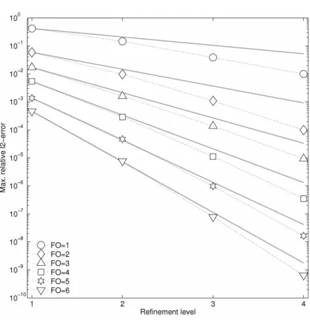
Figure 4.5 shows the maximum relativel2-error over all generated outputs versus

the refinement level of the mesh. The number of coefficients per ray is Nξ = 51 and the time-step is ∆t= 1/160. As a guide to the eye, lines with slopes from one to six are added. All elements converge with the expected rate or better, confirming again that the pole condition does not compromise the order of convergence of the spatial discretization.

Table 4.2 shows the maximum relativel2-error versus the length of the employed

Fig. 4.4. Relative l2-error over time for the Schr¨odinger equation for six different values of

Nξ. The simulation used finite elements of order four, a five times refined mesh and a time-step

∆t= 1/6000.

From ∆t = 1/10 to ∆t = 1/20, a slightly reduced convergence rate is observed, probably because the time-step size is still in the pre-asymptotic regime. The reduced convergence rate in the last refinement is because the error approaches the spatial discretization error, see Figure 4.5. Beside that, the expected fifth order convergence is observed, demonstrating that the pole condition can not only preserve the accuracy of high order finite elements but also of high order integration schemes.

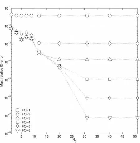
Figures 4.6 and 4.7 show the relative l2-error versus the number of coefficients Nξ. The former shows the maximum error over all outputs for finite elements of order one to six, a three times refined mesh and a time-step ∆t = 1/160. In contrast to Schr¨odinger’s equation, for small values ofNξ there is only a minor decrease of the error. Also, belowNξ, the error is not decreasing monotonically with the number of coefficients. After Nξ = 10, rapid super-algebraically decrease of the error is again observed until the error saturates at a level determined by the accuracy of the spatial discretization. Note that Nξ = 30 coefficients per ray are sufficient here to reduce the boundary condition error to the level of the spatial discretization error in all cases. Figure 4.7 shows the relative error at four different points in time. Again the error generally decays super-algebraically with the number of coefficients, but now the decay rates are noticeably lower at later points in time. Note that att= 0.43, the Gauss peak has not yet reached the boundary, so that the boundary condition has no visible effect on the error at this time.

Fig. 4.5. Verification of the spatial order of convergence for the drift-diffusion equation inte-grated untilT= 5. Shown is the maximum of the relativel2-errors over all generated outputs. The

number of coefficients per ray isNξ= 51and the time-step is∆t= 1/160.

only for larger values of Nξ a significantly reduced error is observed at the end of the simulation. Together with Figure 4.6, this illustrates that for the drift-diffusion example, the error is not monotonically decreasing withNξfor small values ofNξand a certain minimum number of coefficients per ray is required before the onset of the super-algebraic decay.

4.3. Wave and Klein-Gordon equation. For p(∂t) = ∂tt and d = (0,0)T, (1.1) becomes the Klein-Gordon equation, containing the wave equation as the special case k = 0. While the pole condition could successfully provide TBCs for both equations in the one-dimensional case as well as in a two-dimensional wave-guide problem, stability problems arise in the fully two-dimensional case, rendering the pole condition in the here presented form inapplicable to both equations for finite elements of order two or higher. Resolving these issues is planned for future research.

Below, the instability is documented briefly. Use an initial distribution

u(x, y) = exp −2x2−2y2

, (4.5)

finite elements of order one to four and up to four refinement steps for the mesh. Integrate in time using implicit trapezoidal rule with a time-step ∆t= 1/1280 until

T = 100.

Figure 4.9 shows the maximuml2-error over all generated outputs versus the size

of the elements of the employed mesh for finite elements of order one to four. In order to obtain a readable plot, the error is capped at 101_{and values of 10 correspond}

Fig. 4.6. Relativel2-error depending on the number of coefficientsNξ per ray in the exterior

domain for the drift-diffusion equation. Maximum error over all generated outputs for finite elements of order one to six on a three times refined mesh.

two refinement steps. Note that on the coarser meshes where the method is stable, the expected or better decay rates of the error are observed. Similar behavior is found for the Klein-Gordon equation, but not documented here.

Figure 4.10 shows the energy of the discrete solution over time for different values ofNξ on the finest mesh for finite elements of order two. The simulations are stable for Nξ = 4. They are also stable until about t = 20 for Nξ = 6,10,12,15, but an exponential instability occurs after this point in time. The instability also occurs when the simulation is run on a circular domain. Note that the employed integration scheme is A-stable, so that the instability on a finer mesh is not arising from a violation of some CFL-type stability limit.

5. Conclusions. The pole condition approach to transparent boundary condi-tions, derived in [18] for the time-dependent, one-dimensional case, is extended to time-dependent two-dimensional problems. The pole condition identifies in- and out-going modes by associating them with poles of the spatial Laplace transform in the complex plane. The complex plane is then divided into two half-planes, C_{in and} C_{out, containing the poles corresponding to incoming and outgoing modes}

respec-tively. To suppress modes traveling from the exterior into the computational domain, the Laplace transform is required to be analytic inC_{in. In order to obtain a}

numer-ically implementable formulation, C_{in is mapped to the unit circle by a conformal}

M¨obius transformation. The Laplace transform is then extended in a power series on the unit circle with the coefficients of the expansion being connected to the interior degrees of freedom on the boundary. Truncating the series after a finite number of terms yields an approximate and implementable TBC.

Fig. 4.7.Relativel2-error depending onNξat four fixed points in time for the simulation with

finite elements of order six. In all cases, a time-step∆t= 1/160has been used.

different well-known equations for specific choices of parameters. Excellent results are obtained for Schr¨odinger’s equation and the drift-diffusion equation: The presented numerical experiments demonstrate that the convergence order of finite elements up to order six is retained and also that the convergence order of the temporal discretization is not affected if sufficiently many coefficients are used for the boundary condition. Further it is shown that the error introduced by the approximate boundary condition decays super-algebraically as the number of coefficients in the expansion of the Laplace transform increases. For the drift-diffusion equation, a small minimal number of coefficients was found to be required to reach the regime of super-algebraic error decay.

Unfortunately, in contrast to the one-dimensional case, the approach exhibits instabilities for the two-dimensional wave and Klein-Gordon equation if using finite elements of order two or higher. Hence in the present form the pole condition is of limited use for these second order hyperbolic equations. A further investigation of the instability and hopefully a remedy will be subject of future research.

REFERENCES

[1] B. Alpert, L. Greengard, and T. Hagstrom,Rapid evaluation of nonreflecting boundary kernels for time-domain wave propagation, SIAM J. Numer. Anal., 37 (2000), pp. 1138– 1164.

[2] X. Antoine, A. Arnold, C. Besse, M. Ehrhardt, and A. Sch¨adle, A review of trans-parent and artificial boundary conditions techniques for linear and nonlinear Schr¨odinger equations, Commun. Comput. Phys., 4 (2008), pp. 729–796.

[3] R. Astley, Infinite elements for wave problems: A review of current formulations and an assessment of accuracy., Int. J. Numer. Methods Eng., 49 (2000), pp. 951–976.

Fig. 4.8. Relativel2-error over time for the drift-diffusion equation for different values ofNξ

at a four times refined mesh, finite elements of order six and a time-step∆t= 1/160.

[5] B. Engquist and A. Majda,Absorbing boundary conditions for the numerical simulation of waves, Math. Comp., 31 (1977), pp. 629–651.

[6] M. Gander and A. Sch¨adle,The pole condition: A Pad´e approximation of the Dirichlet to Neumann operator, in Domain decomposition methods in Science and Engineering XV, Lecture Notes in Computational Science and Engineering, Springer Verlag, 2010. [7] D. Givoli,Non-reflecting boundary conditions, J. Comput. Phys., 94 (1991), pp. 1–29. [8] ,High-order local non-reflecting boundary conditions: a review, Wave Motion, 39 (2004),

pp. 319–326.

[9] T. Hagstrom,Radiation boundary conditions for numerical simulation of waves, Acta Nu-merica, 8 (1999), pp. 47–106.

[10] E. Hairer and G. Wanner, Solving Ordinary Differential Equations II, Springer Verlag, Berlin, Heidelberg, 1991.

[11] T. Hohage and L. Nannen,Hardy space infinite elements for scattering and resonance prob-lems, SIAM J. Numer. Anal., 47 (2009), pp. 972–996.

[12] T. Hohage, F. Schmidt, and L. Zschiedrich,Solving Time-Harmonic Scattering Problems Based on the Pole Condition I: Theory, SIAM J. Math. Anal., 35 (2003), pp. 183–210. [13] ,Solving Time-Harmonic Scattering Problems Based on the Pole Condition II:

Conver-gence of the PML Method, SIAM J. Math. Anal., 35 (2003), pp. 547–560.

[14] B. Kettner and F. Schmidt,Meshing of heterogeneous unbounded domains, in Proceedings of the 17th Int. Meshing Roundtable, R. V. Garimella, ed., Springer, 2008.

[15] E. Lindman,Free-space boundary conditions for the time dependent wave equation, Journal of Computational Physics, 18 (1975), pp. 66 – 78.

[16] L. Nannen,Hardy-Raum Methoden zur numerischen L¨osung von Streu- und Resonanzproble-men auf unbeschr¨ankten Gebieten, dissertation, Georg-August-Universit¨at zu G¨ottingen, 2008.

[17] L. Nannen and A. Sch¨adle,Hardy space infinite elements for Helmholtz-type problems with unbounded inhomogeneities, Wave Motion, 48 (2011).

[18] D. Ruprecht, A. Sch¨adle, F. Schmidt, and L. Zschiedrich,Transparent boundary condi-tions for time-dependent problems, SIAM J. Sci. Comput., 30 (2008), pp. 2358–2385. [19] F. Schmidt,Solution of Interior-Exterior Helmholtz-Type Problems Based on the Pole

Condi-tion Concept: Theory and Algorithms, habilitation thesis, Freie Universit¨at Berlin, Fach-bereich Mathematik und Informatik, 2002.

Fig. 4.9. Spatial order of convergence for the wave equation integrated untilT = 100. Shown is the maximuml2-error over all generated outputs. The error is capped at101, so depicted error

values of10correspond to unstable runs.

solution of Fresnel’s equation, Comput. Math. Appl., 29 (1995), pp. 53–76.

[21] F. Schmidt, T. Hohage, R. Klose, A. Sch¨adle, and L. Zschiedrich,Pole condition: A numerical method for Helmholtz-type scattering problems with inhomogeneous exterior do-main, J. Comp. Appl. Math., 218 (2008), pp. 61–69.

[22] F. Schmidt and D. Yevick,Discrete transparent boundary conditions for Schr¨odinger-type equations, J. Comput. Phys., 134 (1997), pp. 96–107.

[23] S. Tsynkov,Numerical solution of problems on unbounded domains. A review, Applied Nu-merical Mathematic, 27 (1998), pp. 465–532.

[24] L. Zschiedrich,Transparent Boundary Conditions for Maxwell’s Equations: Numerical Con-cepts beyond the PML Method, dissertation, FB Mathematik, Freie Universit¨at Berlin, 2009.

Fig. 4.10. Energy over time for the wave equation for different values ofNξ. The refinement