White Rose Research Online
Universities of Leeds, Sheffield and York
http://eprints.whiterose.ac.uk/
This is a copy of the final published version of a paper published via gold open access
in
Medical Decision Making
.
This open access article is distributed under the terms of the Creative Commons
Attribution Licence (
http://creativecommons.org/licenses/by/3.0
), which permits
unrestricted use, distribution, and reproduction in any medium, provided the
original work is properly cited.
White Rose Research Online URL for this paper:
http://eprints.whiterose.ac.uk/78429
Published paper
Strong, M and Oakley, JE (2013) An Efficient Method for Computing
Parameter Partial Expected Value of Perfect
Information
Mark Strong, PhD, Jeremy E. Oakley, PhD
The value of learning an uncertain input in a decision model can be quantified by its partial expected value of perfect information (EVPI). This is commonly estimated via a 2-level nested Monte Carlo procedure in which the parameter of interest is sampled in an outer loop, and then conditional on this sampled value, the remaining pa-rameters are sampled in an inner loop. This 2-level method can be difficult to implement if the joint distribu-tion of the inner-loop parameters condidistribu-tional on the parameter of interest is not easy to sample from. We
present a simple alternative 1-level method for calculating partial EVPI for a single parameter that avoids the need to sample directly from the potentially problematic condi-tional distributions. We derive the sampling distribution of our estimator and show in a case study that it is both statistically and computationally more efficient than the 2-level method. Key words: expected value of perfect information; economic evaluation model; Monte Carlo methods; Bayesian decision theory; computational meth-ods; correlation(Med Decis Making 2013;33:755–766)
T
he value of learning an input to a decision-analytic model can be quantified by its partial expected value of perfect information (partial EVPI).1–4 The partial expected value of information for some model input,Xi, is the expected difference between the value of the optimal decision based on perfect information aboutXi and the value of the deci-sion made only with prior information. To express this formally, we first introduce some notation.We assume that we are faced with D decision options, indexedd= 1, . . .,D, and have built a model
yd5fðd;xÞthat aims to predict the net benefit of deci-sion optiondgiven a vector of input parameter values
x. We denote the true unknown values of the inputs
X5fX1;. . .;Xpg, and the uncertain net benefit under decision optiondasYd. We denote the input
param-eter for which we wish to calculate the partial EVPI as Xi and the remaining input parameters as
Xi5fX1;. . .;Xi1;Xi11;. . .;Xpg. We denote the expectation over the full joint distribution of X as
EX, over the marginal distribution ofXi as EXi, and over the conditional distribution ofXijXi asEXijXi.
The expected value of our optimal decision, made only with current information, is
max
d EXffðd;XÞg: ð1Þ
If we knew the value of some input of interest,Xi, then the optimal decision would be that with the greatest net benefit, after averaging over the condi-tional distribution of the remaining unknown inputs,
XijXi. The expected net benefit would be
max
d EXijXiffðd;Xi;XiÞg: ð2Þ But, since Xi is unknown, we must average over our current information aboutXi, giving
EXi max
d EXijXiffðd;Xi;XiÞg
: ð3Þ
The partial EVPI for input Xi is the difference between equation (3), the expected value of the deci-sion made with perfect information about Xi, and equation (1), the expected value of the current opti-mal decision option,3,4
Received 4 October 2011 from School of Health and Related Research (ScHARR), University of Sheffield, UK (MS), and School of Mathematics and Statistics, University of Sheffield, UK (JEO). MS was funded by the UK Medical Research Council fellowship grant G0601721 while under-taking this study. Revision accepted for publication 25 July 2012. Address correspondence to Mark Strong, School of Health and Related Research (ScHARR), University of Sheffield, Regent Court, 30 Regent Street, Sheffield, UK; e-mail: [email protected].
EVPIðXiÞ5EXi max
d EXijXiffðd;Xi;XiÞg
max
d EXffðd;XÞg: ð4Þ
We are commonly in a situation in which we cannot evaluate any of the 3 expectations in equation (4) ana-lytically. Important exceptions are cases in which
models are either of linear form (e.g.,
Y15b1X11b2X2) or multilinear (sum-product) form (e.g., Y15b1X1X21b2X3X4) (where b1 and b2 are constants). In the linear case, the expectation in equa-tion (1) and the inner expectaequa-tion in equaequa-tion (3) both have an analytic solution, and in the multilinear case, these expectations have an analytic solution if inputs are independent. In the case of correlated inputs, ana-lytic solutions to these 2 expectations will sometimes exist, such as the case in which the inputs have a mul-tivariate Normal distribution. The outer expectation in equation (3) is more problematic due to the maxi-mization step, and analytic solutions rarely exist.
In the absence of analytic solutions to the expecta-tions in equation (3), the usual approach is to use a nested 2-level Monte Carlo method. This requires us to sample a value of the input parameter of interest in an outer loop and then to sample values from the joint conditional distribution of the remaining parameters and run the model in an inner loop.5,6 Sufficient numbers of runs of both the outer and inner loops are required to ensure that the partial EVPI is estimated with sufficient precision and with an acceptable level of bias.7
We recognize 2 important practical limitations to the standard 2-level Monte Carlo approach to calcu-lating partial EVPI. First, the nested 2-level nature of the algorithm with a model run at each inner-loop step can be highly computationally demanding for all but very small loop sizes if the model is expen-sive to run. Second, we require a method of sampling from the joint distribution of the inputs (excluding the parameter of interest) conditional on the input parameter of interest. If the input parameter of interest is independent of the remaining parameters, then we can simply sample from the unconditional joint distri-bution of the remaining parameters. However, if inputs are not independent, we may need to resort to Markov chain Monte Carlo (MCMC) methods if there is no ana-lytic solution to the joint conditional distribution. Including an additional MCMC step in the algorithm is likely to increase the computational burden consider-ably, as well as requiring additional programming.
In this article, we present a simple 1-level ‘‘ordered input’’ algorithm for calculating single-parameter
partial EVPI, which requires only a single set of the sampled inputs and corresponding outputs to calcu-late partial EVPI values for all input parameters. The method is applicable in any modeling scenario in which there is no analytic solution to the expecta-tions in equation (4). The method avoids the nested double loop and is therefore computationally less demanding than the standard 2-level method, and it also avoids the need to sample directly from the con-ditional distributions of the inputs when inputs are correlated. We describe methods for quantifying the upward bias and precision of the estimator. We illus-trate the method in a case study with 2 scenarios: a multilinear model in which inputs are correlated, but with known analytic solutions for all conditional distributions, and the same model in which inputs are correlated but where sampling from the condi-tional distributions requires MCMC.
METHODS
In this section, we describe an algorithm for com-puting the partial EVPI for a single input parameter of interest,Xi. Code for implementing the algorithm in R8 is shown in Appendix A and is available for download at http://www.shef.ac.uk/scharr/sections/ ph/staff/profiles/mark.
Briefly, the idea is as follows. We assume we have a set of samples from the joint distribution of the model input parameters and a corresponding set of model outputs (i.e., net benefits). The net benefits (for each decision option) are ordered with respect to the input of interest and then partitioned into subsets of equal size. Within each subset, we calcu-late the mean of the net benefits for each decision option and take the maximum across the decision options. The average of these maxima is taken as an approximation to the first term in equation (4). The second term in equation (4) is computed using stan-dard Monte Carlo sampling—that is, for each deci-sion option, we calculate the mean of the net benefits corresponding to the whole set of input samples and then take the maximum of these means.
In the following subsections, we introduce nota-tion and describe the algorithm in detail in a series of stages.
Stage 1
We define the Monte Carlo sample of model
inputs and corresponding model outputs as
fðxs;ys
drawn from the joint distribution of the inputs,pðXÞ, andys
d5fðd;xsÞis the evaluation of the model output at xs for decision option d. Note the use of super-scripts to index the randomly drawn sample sets. We letMbe the matrix of inputs and corresponding outputs
M5
x1
1 . . . x1p y11 . . . y1D x2
1 . . . x2p y21 . . . y2D .. . .. . .. . .. . .. . .. . xS
1 . . . xSp yS1 . . . ySD 0 B B B B @ 1 C C C C
A: ð5Þ
Stage 2
For parameter of interesti, we extract thexi and
y1;. . .;yD columns and reorder with respect to xi, giving
M5
xði1Þ yð11Þ . . . yðD1Þ xði2Þ yð12Þ . . . yðD2Þ
.. . .. . .. . .. .
xðiSÞ yð1SÞ . . . yðDSÞ 0 B B B B @ 1 C C C C
A; ð6Þ
wherexð1Þi xð2Þi . . .xðiSÞ. Note the use of brack-eted superscripts to denote the sample set ordered with respect to the input of interest.
Stage 3
We partition the resulting matrix intok51;. . .;K
submatricesMðkÞofJrows each,
MðkÞ5
xið1;kÞ y1ð1;kÞ . . . yðD1;kÞ xið2;kÞ y1ð2;kÞ . . . yðD2;kÞ
.. . .. . .. . .. .
xiðJ;kÞ y1ðJ;kÞ . . . yðDJ;kÞ 0 B B B B @ 1 C C C C
A; ð7Þ
retaining the ordering with respect toxi, and where the row indexed (j, k) in equation (7) is the row indexed ðj1ðk1ÞJÞ in equation (6). Note that
J3Kmust equal the total sample sizeS.
Stage 4
For each MðkÞ, we estimate (for each decision
option) the conditional expectationmðdkÞ5E
XijXi5x
ðkÞ
i
fðd;Xi;XiÞ
f gby averaging overj51;. . .;J, that is,
^
mðdkÞ51
J PJ j51
yðdj;kÞ; ð8Þ
wherexði kÞ5PJj51xðij;kÞ=J.
The justification for this rests on recognizing that if Jis small compared withS, then the ordered values of the input of interestnxð1i ;kÞ;. . .;xiðJ;kÞowill all be close to their mean value, xði kÞ, and the corresponding values of the remaining inputs nxð1i;kÞ;. . .;xðJi;kÞo
will be (approximately) a sample from the distribu-tion of XijXi5xði kÞ. See Appendix B for a more for-mal justification.
The maximum mðkÞ5maxd E
XijXi5x
ðkÞ
i
fðd;Xi; f
XiÞgis then estimated by
^
mðkÞ5max
d m^
ðkÞ
d ; ð9Þ
and finally we estimate the first term on the right-hand side of equation (4) by averaging over
k51;. . .;K, that is,
^ m51
K XK
k51 ^
mðkÞ: ð10Þ
Stage 5
We estimate the second term on the right-hand side of equation (4) using simple Monte Carlo sam-pling, that is,
max
d EXffðd;XÞg ’maxd
1
S XS
n51
ynd; ð11Þ
where the order of thexnis irrelevant.
Stages 2 to 4 are repeated for each parameter of interest, noting that only a single set of model runs (stage 1) is required.
CHOOSING VALUES FORJAND K
We assume that we have a fixed number of model evaluationsSand wish to choose values forJandK subject to the constraintJ3K5S.
1
S XS
s51 max
d ðy s
dÞ; ð12Þ
which is the Monte Carlo estimator for the first term in the expression for theoverallEVPI,
EVPI5EX max
d fðd;XÞ
max
d EXffðd;XÞg: ð13Þ
Second, we note that for very large values ofJ, and hence small values ofK, the EVPI estimator is down-wardly biased and converges to zero whenJ=S. In this case, our ordered input estimator for the first term on the right-hand side of equation (4) reduces to
max
d
1
S XS
s51
ys
d; ð14Þ
which is the Monte Carlo estimator for the second term on the right-hand side of Equation 4.
The precision of the partial EVPI estimate only depends on Sand not on J andK(see Appendix C for the derivation of an expression for the variance of the estimator). We therefore only need to consider the minimization of bias in our choice ofJandKwhen S is fixed. Because the upward bias due to small Jconverges to zero asJ increases, a sensible choice ofJis that which is just large enough such that the estimated bias b^ is smaller than some constant c. Any choice ofJlarger than this will risk introducing a downward bias that becomes apparent at small values ofK.
We estimate the upward bias in the following man-ner, using the method proposed by Oakley and others.7First, we write the vector of Monte Carlo esti-mators for the conditional expected net benefits from
equation (8) asm^ðkÞ5m^1ðkÞ;. . .;m^ðDkÞ
9
. If we can deter-mine the sampling distribution of this vector of esti-mators, then we can quantify the upward bias inm^
and hence the upward bias in the partial EVPI. UnlessJis very small,m^ðkÞwill follow a multivariate Normal distribution withDdimensions. Thus, we have
^
mðkÞ;ND mðkÞ;1 JV
ðkÞ
; ð15Þ
where mðkÞ5m1ðkÞ;. . .;mðDkÞ 9
, and where each ele-mentp,qofVðkÞis estimated by
^
Vpðk;qÞ5cov m^
ðkÞ
p ;m^
ðkÞ
q
: ð16Þ
To estimate the bias inm^, we first draw, for each
k51;. . .;K, a set of N samples from a multivariate Normal distribution with mean vectorm^ðkÞ and vari-ance matrix 1
JV^
ðkÞ
p;q. We choose N to be large, say
1000. Let us denote these samples
~
mðnkÞ5m~ð1k;nÞ;. . .;m~Dðk;Þnforn51;. . .;Nandk51;. . .;K. The bias inm^ðkÞis estimated by
^ bðkÞ51
N XN
n51
maxnm~ð1;knÞ;. . .;m~ðDk;Þnomaxnm^ð1kÞ;. . .;m^ðDkÞo;
ð17Þ
and the expected bias inm^ as
^ b51
K XK
k51 ^
bðkÞ: ð18Þ
R code for computing the bias estimate is available for download at http://www.shef.ac.uk/scharr/ sections/ph/staff/profiles/mark.
The left panel of Figure 1 showsb^, the expected upward bias in the partial EVPI for various values of
J(on the log10scale) for inputX6in the first scenario
of the case study outlined later in the article. The total number of model evaluations, S, is 1,000,000, and
K5S=J. Note the convergence to zero asJincreases. The arrow is placed atJ51000, the smallest value of
Jfor which the bias is less than£1.
The right panel shows values for the estimated par-tial EVPI againstJ(on the log10scale). In scenario 1 of the case study, the inner expectation of equation (4) has an analytic solution, and we were therefore able to com-pute a value of the partial EVPI values for all parameters to high precision using a simple 1-level Monte Carlo sampling scheme. This ‘‘analytic’’ value is shown in the figure, as is the overall EVPI for all parameters. The total number of model evaluations S is again 1,000,000, withK5S=J. Note the upward and down-ward biases at extreme values ofJ but also the large region of stability between J5100 (K510;000) and
J5100;000 (K510). The arrow is placed atJ= 1000, the smallest value ofJfor which the bias is less than
£1. At this point, the estimated partial EVPI is £612.63 compared with the analytic value of £612.38.
CASE STUDY
in Brennan and others,5 Oakley and others,7 and Kharroubi and others.9The model predicts monetary net benefit,Yd, under 2 decision options (d51;2) and can be written in sum product form as
Y1 5 lðX5X6X71X8X9X10Þ ðX11X2X3X4Þ; ð19Þ
Y2 5 lðX14X15X161X17X18X19Þ ðX111X12X13X4Þ; ð20Þ
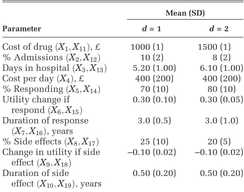
where X5fX1;. . .;X19g are the 19 uncertain input parameters listed in Table 1, and the willingness to pay for 1 unit of health output in quality-adjusted life years (QALYs) isl5£10;000=QALY.
Scenario 1: Correlated Inputs with Known Condi-tional Distributions
In scenario 1, we assume that a subset of the inputs are correlated but with a joint distribution such that we can sample from the conditional distributions of the correlated inputs without the need for MCMC. We assume that the inputs are jointly Normally dis-tributed, withX5,X7,X14, andX16all pairwise
corre-lated with a correlation coefficient of 0.6 and with all other inputs independent. In a simple sum product form model, the assumption of multivariate Normal-ity allows us to compute the inner conditional expec-tation analytically, as well as allowing us to sample
directly from the conditional distribution XijXi in the standard nested 2-level method, but this will not necessarily be the case in models with additional nonlinearity.
We calculated partial EVPI using 3 methods. First, we calculated the partial EVPI for each parameter using a single-loop Monte Carlo approximation for the outer expectation in the first term of the right-hand side of equation (4) with 106samples from the distribution of the parameter of interest, as well as an analytic solution to the inner conditional expecta-tion. Next, we calculated the partial EVPI values using the standard 2-level Monte Carlo approach with 1000 inner-loop samples and 1000 outer-loop samples (i.e., 10003 1000 = 106model evaluations in total). Finally, we computed the partial EVPI values using the ordered sample method with the same number of model evaluations, S5106, and
values ofJ=K= 1000.
Standard errors and bias estimates for the 2-level Monte Carlo partial EVPI estimates were obtained using the methods presented in Oakley and others.7 The standard errors for the ordered input method partial EVPI estimates were obtained using the method presented in Appendix C. The bias mates for the ordered input method partial EVPI esti-mates were obtained using the method presented in the Methods section above. We measured the total computation time for obtaining EVPI values for all 19 parameters.
0 1 2 3 4 5 6
0
2
00
400
600
8
00
1000
1200
log10(J)
upward bias (£)
0 1 2 3 4 5 6
0
2
00
400
600
8
00
1000
1200
log10(J)
partial EVPI (£)
Estimated partial EVPI Overall EVPI
[image:6.594.53.545.91.303.2]‘Analytic’ value for partial EVPI
Figure 1 Left panel: upwards bias in partial expected value of perfect information (EVPI) estimator against log10J. Right panel: estimated
partial EVPI at values ofJranging from 1 to106where the total number of model evaluations,S, is106. The arrows show the smallest value
Results for Scenario 1.Calculating the expected net benefits for decision options 1 and 2 analytically results in values of£5057.00 and £5584.80, respec-tively, indicating that decision option 2 is optimal. Running the model with 106 Monte Carlo samples
from the joint distribution of the input parameters results in option 2 having greater net benefit than option 1 in only 54% of samples, suggesting that the input uncertainty is resulting in considerable decision uncertainty. The overall EVPI is£1046.10. The partial EVPI values for parametersX1toX4,X8
to X13, andX17 to X19 were all less than £0:01 and therefore considered unimportant in terms of driving the decision uncertainty. Results for the remaining parameters are shown in Table 2. The standard errors of the partial EVPI values estimated via the ordered input method are considerably smaller than those estimated via the 2-level method, whereas the esti-mated bias for each parameter is similar. The ordered input method is approximately 4 times faster than the standard 2-level Monte Carlo method in this case.
Scenario 2: Correlated Inputs with Conditional Distribution Sampling Requiring MCMC
In scenario 2, we assume that a subset of the inputs are correlated but with a joint distribution such that we can only sample from the conditional distribu-tions of the correlated inputs using MCMC. We assume, as in scenario 1, that X5, X7, X14, and X16
are pairwise correlated, but with a more complicated dependency structure based on an unobserved
bivariate Normal latent variableZ5ðZ1;Z2Þthat has expectation zero, variance 1, and correlation 0.6. Conditional on this latent variable, which represents some measure of effectiveness, the proportions of responders (X5andX14) are assumed beta distributed
and the durations of response (X7andX16) assumed gamma distributed. The hyperparameters of the beta and gamma distributions are defined in terms of Z such that X5, X7, X14, andX16 have the means and
standard deviations in Table 1.
We calculated partial EVPI for each parameter using the standard 2-level Monte Carlo approach with 1000 inner-loop samples and 1000 outer-loop samples (i.e., 10003 1000 = 106model evaluations in total) using OpenBUGS10to sample from the con-ditional distribution ofXijXi. Finally, we computed the partial EVPI values using the ordered sample method with the same number of model evaluations,
S5106, and values ofJ=K= 1000.
Results for Scenario 2.Running the model with106
samples from the joint distribution of the input param-eters resulted in expected net benefits of£5043.12 and
£5549.93 for decision options 1 and 2, respectively, indicating that decision option 2 is optimal, but again with considerable decision uncertainty. Based on this sample, the probability that decision 2 is best is 54%, and the overall EVPI is£1240.33.
Partial EVPI results are shown in Table 3. Values for parameters X1 to X4, X8 to X13, and X17 to X19
were again all less than £0:01 and are not shown. Standards errors for the partial EVPI values estimated via the ordered input method are again smaller than those estimated via the 2-level method. The esti-mated bias is marginally smaller for the ordered input method. The ordered input method is approximately 800 times faster than the 2-level Monte Carlo/MCMC method in this case.
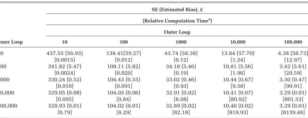
How Many 2-Level Monte Carlo Inner- and Outer-Loop Samples Are Required to Achieve a Bias and Precision Similar to the Ordered Input Method?
We compared the bias and precision of the partial EVPI estimated via the ordered method with that esti-mated via the 2-level method with a range of inner-and outer-loop sizes. Our comparator was the partial EVPI for input parameterX6for scenario 1 computed
[image:7.594.46.288.107.298.2]using the ordered 1-level method with a total sample size of106andJ=K= 1000. Using this method, the upward bias was estimated to be£0.50, and the stan-dard error of the estimate was£3.15 (Table 2). Table 4 shows the bias and standard error for the 2-level Table 1 Summary of Input Parameters
Mean (SD)
Parameter d= 1 d= 2
Cost of drugðX1;X11Þ, £ 1000 (1) 1500 (1)
% AdmissionsðX2;X12Þ 10 (2) 8 (2)
Days in hospitalðX3;X13Þ 5.20 (1.00) 6.10 (1.00)
Cost per dayðX4Þ, £ 400 (200) 400 (200)
% RespondingðX5;X14Þ 70 (10) 80 (10)
Utility change if
respondðX6;X15Þ
0.30 (0.10) 0.30 (0.05)
Duration of response
ðX7;X16Þ, years
3.0 (0.5) 3.0 (1.0)
% Side effectsðX8;X17Þ 25 (10) 20 (5)
Change in utility if side
effectðX9;X18Þ
–0.10 (0.02) –0.10 (0.02)
Duration of side
effectðX10;X19Þ, years
Monte Carlo method for different inner- and outer-loop sizes, which were estimated using the method proposed by Oakley and others.7The reported com-putation times are relative to the time taken for the
ordered input method with a sample size of106and
J=K= 1000.
[image:8.594.44.546.110.225.2]To achieve a similar precision and bias via the 2-level Monte Carlo method, the outer loop must be of Table 2 Partial Expected Value of Perfect Information (EVPI) Values for Scenario 1
Partial EVPI (SE; Estimated Bias), £
Parameter Analytic Conditional Expectation Two-Level Monte Carlo Ordered Input Method
X5 22.50 9.52 (65.20; 1.85) 25.29 (3.26; 1.62)
X6 612.38 614.76 (33.02; 0.46) 612.63 (3.15; 0.50)
X7 11.56 77.65 (66.38; 1.31) 14.86 (3.28; 1.61)
X14 230.94 312.39 (69.59; 1.55) 233.63 (3.19; 1.42)
X15 271.52 315.02 (29.52; 1.45) 273.00 (3.30; 1.17)
X16 458.97 502.91 (77.98; 0.85) 462.42 (3.12; 0.65)
Computation timea 4.2 1
[image:8.594.55.546.264.385.2]aComputation time is the total time to compute the partial EVPI for all 19 input parameters and is reported relative to the ordered input method.
Table 3 Partial Expected Value of Perfect Information (EVPI) Values for Scenario 2
Partial EVPI (SE; Bias), £
Parameter Two-Level Monte Carlo with MCMC Inner Loop Ordered Input Method
X5 102.55 (34.48; 3.82) 34.65 (3.26; 0.82)
X6 610.82 (38.02; 0.93) 618.80 (3.10; 0.78)
X7 132.16 (36.10; 4.57) 56.25 (3.25; 0.81)
X14 334.13 (51.94; 1.43) 368.87 (3.18; 0.77)
X15 223.09 (25.73; 2.04) 275.78 (3.25; 0.82)
X16 554.20 (64.00; 0.89) 663.25 (3.13; 0.80)
Computation timea 810 1
MCMC, Markov chain Monte Carlo.
aComputation time is the total time to compute the partial EVPI for all 19 input parameters and is reported relative to the ordered input method.
Table 4 Standard Error and Bias for ParameterX6in Scenario 1, Computed via the 2-level Monte Carlo Method for a Range of Inner- and Outer-Loop Sizes
SE (Estimated Bias), £
[Relative Computation Timea] Outer Loop
Inner Loop 10 100 1000 10,000 100,000
[image:8.594.53.544.441.629.2]10 437.55 (56.93) 138.41(59.27) 43.74 (58.38) 13.84 (57.70) 4.38 (58.73)
[0.0015] [0.012] [0.12] [1.24] [12.97]
100 341.82 (5.47) 108.11 (5.82) 34.18 (5.46) 10.81 (5.56) 3.42 (5.61)
[0.0024] [0.020] [0.19] [1.96] [20.59]
1000 330.24 (0.52) 104.43 (0.55) 33.02 (0.46) 10.44 (0.67) 3.30 (0.47)
[0.010] [0.091] [0.93] [9.38] [99.91]
10,000 329.05 (0.08) 104.05 (0.06) 32.91 (0.02) 10.41 (0.07) 3.29 (0.01)
[0.095] [0.84] [8.08] [80.92] [801.53]
100,000 328.93 (0.01) 104.02 (0.01) 32.89 (0.02) 10.40 (0.02) 3.29 (0.01)
[0.79] [8.29] [82.18] [819.93] [8139.48]
the order of 100,000 and the inner loop of the order of 1000. This therefore requires108 model evaluations
and is approximately 100 times slower to compute than the ordered input method.
DISCUSSION
We have presented a method for calculating the partial expected value of perfect information that is simple to implement, is rapid to compute, and does not require an assumption of independence between inputs. The saving in computational time is particu-larly marked if the alternative is to use a nested 2-level EVPI approach in which the conditional expectations are estimated using MCMC. The method is straightforward to apply in a spreadsheet applica-tion, even with little programming knowledge.
Our approach requires only a single set of model evaluations to calculate partial EVPI for all inputs, allowing a complete separation of the EVPI calcula-tion step from the model evaluacalcula-tion step. This sepa-ration may be particularly useful when the model has been evaluated using specialist software (e.g., for discrete event or agent-based simulation) that does not allow easy implementation of the EVPI step or when those who wish to compute the EVPI do not ‘‘own’’ (and therefore cannot directly evalu-ate) the model. The method does require that, if any inputs are correlated, the inputs are sampled from their joint distribution, rather than from their separate marginal distributions. However, this is unlikely to be an important limitation. When inputs are correlated, sampling from their joint distribution is usual practice, for example, when sampling Dirichlet distributed transition probabilities or multivariate Normal distributed regression parameters.
As presented, the method calculates the partial EVPI for single inputs one at a time. We may, how-ever, wish to calculate the value of learning groups of inputs simultaneously. There are good reasons for this. First, for certain forms of model, we may find that learning single inputs alone has little value, but learning a group of inputs has high value due to the interactions between those inputs within the model. It is important to note that interactions result from nonadditive effects within the model and can occur even if inputs are uncorrelated. Second, a cer-tain subset of model inputs may be derived from a sin-gle study, and therefore learning one input in this set (by conducting the ‘‘perfect’’ study) implies learning them all. If we are considering the value of a study in
reducing uncertainty about inputs, we will consider the value ofallthe information that arises from the study, not just the information that informs a single input. The value of our method may then be in dril-ling down to specific inputs or small groups of inputs within some larger group of inputs that is judged to be policy relevant. If inputs can be partitioned into broad policy-relevant groups (i.e., those that might be considered together when a decision is made to commission further research), and if these groups can be treated as uncorrelated, then calculating the EVPI for each group of inputs using 2-level Monte Carlo methods is straightforward. At this point, the ordered approximation method could be used to compute the value of single inputs (or small groups of inputs) if this was felt necessary.
Although it is possible to extend our approach to groups of inputs, we quickly come up against the ‘‘curse of dimensionality.’’ This is because the method relies on partitioning the input space into a large number of ‘‘small’’ sets such that in each set, the parameter of interest lies close to some value. This works well where there is a single parameter of interest, but if we wish to calculate the EVPI for a group of parameters, the samples quickly become much more sparsely located in the higher dimen-sional space. Given a single parameter of interest, imagine that we obtain adequate precision if we par-tition the input space intoK= 1000 sets ofJ= 1000 samples each. With 2 parameters of interest, we would need to order and partition the space in 2 dimensions, meaning that to retain the same marginal probabilistic ‘‘size’’ for each set, we now require
K251;000;000 sets of J = 1000 samples each. For
groups of inputs, the standard 2-level approach may be more efficient or, if this is impractical, an alterna-tive such as emulation.11,12
We show in Appendix A that the approximation method relies on the smoothness of the function
gðXi;xi;XiÞ5fðXi;XiÞpðpXðXijXijiX5xiÞ
fðXi;XiÞorpðXijXiÞis not smooth with respect to
Xi, then additional exploration would be warranted before our method is employed.
In conclusion, the ordered sample method for cal-culating partial EVPI is simple enough to be easily implemented in a range of software applications
commonly used in cost-effectiveness modeling, reduces computation time considerably when com-pared with the standard 2-level Monte Carlo approach, and avoids the need for MCMC in nonlin-ear models with awkward input parameter depen-dency structures.
APPENDIX A
R Code for Implementing the Algorithm
The partial.evpi.function function as written below takes as inputs the costs and effects rather than the net benefits. This allows the partial EVPI to be calculated at any value of willingness to pay,l.
partial.evpi.function<-function(inputs,input.of.interest,costs,effects,lambda,J,K)
{
S <- nrow(inputs) # number of samples
if(J*K!=S) stop("The number of samples does not equal J times K")
D <- ncol(costs) # number of decision options
nb <- lambda*effects-costs
baseline <- max(colMeans(nb))
perfect.info <- mean(apply(nb,1,max))
evpi <- perfect.info-baseline
sort.order <- order(inputs[,input.of.interest])
sort.nb <- nb[sort.order,]
nb.array <- array(sort.nb,dim=c(J,K,D))
mean.k <- apply(nb.array,c(2,3),mean)
partial.info <- mean(apply(mean.k,1,max))
partial.evpi <- partial.info-baseline
partial.evpi.index <- partial.evpi/evpi
return(list(
baseline = baseline,
perfect.info = perfect.info,
evpi = evpi,
partial.info = partial.info,
partial.evpi = partial.evpi,
partial.evpi.index = partial.evpi.index
))
APPENDIX B
Theoretical Justification for the Algorithm
The ordered algorithm is a method for efficiently computing the inner expectation in the first term of the right-hand side in equation (4). Dropping the decision option indexdfor clarity but without loss of generality, our target is EXijXi5xiffðx
i;XiÞg where xi is a realized value of the parameter of interest, and Xi are the remaining (uncertain) parameters with joint conditional distributionpðXijXi5xiÞ.
Given a samplenxð1Þi;. . .;xðJiÞofrompðXijXi5xiÞ, the Monte Carlo estimator forEXijXi5xiffðx
i;XiÞgis
^
EXijXi5xiffðx
i;XiÞg5
1
J XJ
j51
f x
i;x
ðjÞ
i
: ð21Þ
In our ordered approximation method, we replace equation (21) with
^
EXijXi5xiffðx
i;XiÞg5
1
J XJ
j51
f xi1ej;x~ðjÞi
; ð22Þ
wherefx
i1e1;. . .;xi1eJg5fxð1Þi ;. . .;xðiJÞgis an ordered sample frompðXijXi2 ½xi6zÞfor some smallz(and thereforee’0), andx~ðjÞi is a sample frompðXijXi5xi1ejÞ
Equation (22) is an unbiased Monte Carlo estimator of
EXi2½xi6z EXijXifðXi;XiÞ
5
ð
Xi
ð
Xi
fðXi;XiÞpðXijXiÞpðXijXi2 ½xi6zÞdXidXi; ð23Þ
which we can rewrite by introducing an importance sampling ratio as
ð
Xi
ð
Xi
fðXi;XiÞpðXijXiÞpðXijXi2 ½xi6zÞdXidXi
5
ð
Xi
ð
Xi
fðXi;XiÞ
pðXijXiÞpðXijXi2 ½xi6zÞ pðXijXiÞpðXijXi5xiÞ
pðXijXiÞpðXijXi5xiÞdXidXi
5
ð
Xi
ð
Xi
fðXi;XiÞ
pðXijXiÞ pðXijXi5xiÞ
pðXijXi2 ½xi6zÞdXipðXijXi5xiÞdXi:
ð24Þ
We write the termsfðXi;XiÞpðpXðXijXijiX5xiÞ
iÞwithin the inner integral as a function
gðÞ, that is,
fðXi;XiÞ
pðXijXiÞ pðXijXi5xiÞ
5gðXi;x
i;XiÞ:
IfgðÞis approximately linear in the small intervalXi2 ½xi6z, then we can expressgðXi;xi;XiÞas a first-order Taylor series expansion aboutgðx
i;xi;XiÞ, giving
fðXi;XiÞ
pðXijXiÞ pðXijXi5xiÞ
5 gðXi;xi;XiÞ;
’ g x
i;xi;Xi
1ðXix
iÞ
qg Xi;x
i;Xi
qXi jXi5xi 5 fðx
i;XiÞ1ðXixiÞ
qg Xi;x
i;Xi
qXi jXi5xi:
Substituting back into equation (24) withc5qg Xi;x
i;Xi
ð Þ
ð
Xi
ð
Xi
fðXi;XiÞ
pðXijXiÞ pðXijXi5xiÞ
pðXijXi2 ½xi6zÞdXipðXijXi5xiÞdXi
’ ð
Xi
ð
Xi
fðx
i;XiÞ1cðXixiÞ
pðXijXi2 ½x
i6zÞdXipðXijXi5xiÞdXi:
SinceÐXicðXixiÞpðXijXi2 ½xi6zÞdXi5EXi2½xi6zfcðXix
iÞg ’0and
Ð
XipðXijXi2 ½x
i6zÞdXi51, then
ð
Xi
ð
Xi
fðxi;XiÞ1cðXixiÞ
pðXijXi2 ½xi6zÞdXipðXijXi5xiÞdXi;
5
ð
Xi
fðx
i;XiÞpðXijXi5xiÞdXi;
5EXijXi5xiffðx
i;XiÞg:
Hence, we have shown that as long asgðXi;xi;XiÞ5fðXi;XiÞpðpXðXijXijiX5xiÞiÞis sufficiently smooth such that it is approximately linear in some small intervalXi2 ½xi6z, the ordered approximation method (equation (22)) will provide a good estimate of our target conditional expectationEXijXi5xiffðx
i;XiÞg.
APPENDIX C
Estimating the Variance of the First Term in the Partial EVPI Estimator
Here we derive an expression for the variance ofm^, the first term in the estimator for the partial EVPI (equa-tion (4)).
If we denotedk5arg maxdm^ðdkÞ, we can rewrite equation (10) as
^ EXiðm^
ðkÞÞ5m^ 5 1
K XK
k51 ^ mðkÞ
5 1
K XK
k51 ^
mðdkÞ
k
5 1
K XK
k51
1
J XJ
j51
yðdj;kÞ
k
!
5 1
S XK
k51 XJ
j51
yðdj;kÞ
k
:
ð25Þ
The variance ofm^is
varðm^Þ 5 var 1
S XK
k51 XJ
j51
yðdj;kÞ
k
!
5 1
S2 XK
k51 XJ
j51
var yðdj;kÞ
k
;
ð26Þ
since theyðdj;kÞ
k are independent. The estimator for varð
^
mÞis therefore simply
d
varðm^Þ 5 1
SðS1Þ XK
k51 XJ
j51
yðdj;kÞ
k m^
2
We see therefore that the precision of the first term in the partial EVPI estimator does not depend on the individual choices ofJandKbut only onS5J3K. Assuming that the second term in the expression for the partial EVPI (equation (4)) is estimated to a high precision by simple 1-level Monte Carlo, then the var-iance of the partial EVPI is approximately equal to the variance of the first term,dvarðm^Þ.
R code for computing the variance estimate is available for download at http://www.shef.ac.uk/ scharr/sections/ph/staff/profiles/mark.
REFERENCES
1. Raiffa H. Decision Analysis: Introductory Lectures on Choices under Uncertainty. Reading, MA: Addison-Wesley; 1968. 2. Claxton K, Posnett J. An economic approach to clinical trial design and research priority-setting. Health Econ. 1996;5(6): 513–24.
3. Felli JC, Hazen GB. Sensitivity analysis and the expected value of perfect information. Med Decis Making. 1998;18(1):95–109. 4. Felli JC, Hazen GB. Erratum: Correction: sensitivity analysis and the expected value of perfect information. Med Decis Making. 2003;23(1):97.
5. Brennan A, Kharroubi S, O’Hagan A, Chilcott J. Calculating par-tial expected value of perfect information via Monte Carlo sam-pling algorithms. Med Decis Making. 2007;27(4):448–70. 6. Koerkamp BG, Myriam Hunink MG, Stijnen T, Weinstein MC. Identifying key parameters in cost-effectiveness analysis using value of information: a comparison of methods. Health Econ. 2006;15(4):383–92.
7. Oakley JE, Brennan A, Tappenden P, Chilcott J. Simulation sam-ple sizes for Monte Carlo partial EVPI calculations. J Health Econ. 2010;29(3):468–77.
8. R Development Core Team. R: A Language and Environment for Statistical Computing. Vienna, Austria: R Development Core Team; 2012. Available from: http://www.R-project.org/
9. Kharroubi SA, Brennan A, Strong M. Estimating expected value of sample information for incomplete data models using Bayesian approximation. Med Decis Making. 2011;31(6):839–52.
10. Lunn D, Spiegelhalter D, Thomas A, Best N. The BUGS project: evolution, critique, and future directions. Stat Med. 2009;28: 3049–67.
11. Oakley JE, O’Hagan A. Probabilistic sensitivity analysis of complex models: a Bayesian approach. J R Stat Soc B. 2004;66(3): 751–69.