Four theorems on the psychometric function

City, University of London Institutional Repository

Citation:

May, K. A. and Solomon, J. A. (2013). Four theorems on the psychometric

function. PLoS One, 8(10), doi: 10.1371/journal.pone.0074815

This is the unspecified version of the paper.

This version of the publication may differ from the final published

version.

Permanent repository link:

http://openaccess.city.ac.uk/2861/

Link to published version:

http://dx.doi.org/10.1371/journal.pone.0074815

Copyright and reuse: City Research Online aims to make research

outputs of City, University of London available to a wider audience.

Copyright and Moral Rights remain with the author(s) and/or copyright

holders. URLs from City Research Online may be freely distributed and

linked to.

Keith A. May*, Joshua A. Solomon

Division of Optometry and Visual Science, City University London, London, United Kingdom

Abstract

In a 2-alternative forced-choice (2AFC) discrimination task, observers choose which of two stimuli has the higher value. The psychometric function for this task gives the probability of a correct response for a given stimulus difference,Dx. This paper proves four theorems about the psychometric function. Assuming the observer applies a transducer and adds noise, Theorem 1 derives a convenient general expression for the psychometric function. Discrimination data are often fitted with a Weibull function. Theorem 2 proves that the Weibull ‘‘slope’’ parameter,b, can be approximated bybNoise|bTransducer, wherebNoiseis thebof the Weibull function that fits best to the cumulative noise distribution, andbTransducerdepends on the transducer. We derive general expressions forbNoiseandbTransducer, from which we derive expressions for specific cases. One case that follows naturally from our general analysis is Pelli’s finding that, when d’!(Dx)b, b&bNoise|b. We also consider two limiting cases. Theorem 3 proves that, as sensitivity improves, 2AFC performance will usually approach that for a linear transducer, whatever the actual transducer; we show that this does not apply at signal levels where the transducer gradient is zero, which explains why it does not apply to contrast detection. Theorem 4 proves that, when the exponent of a power-function transducer approaches zero, 2AFC performance approaches that of a logarithmic transducer. We show that the power-function exponents of 0.4–0.5 fitted to suprathreshold contrast discrimination data are close enough to zero for the fitted psychometric function to be practically indistinguishable from that of a log transducer. Finally, Weibullbreflects the shape of the noise distribution, and we used our results to assess the recent claim that internal noise has higher kurtosis than a Gaussian. Our analysis ofbfor contrast discrimination suggests that, if internal noise is stimulus-independent, it has

lowerkurtosis than a Gaussian.

Citation:May KA, Solomon JA (2013) Four Theorems on the Psychometric Function. PLoS ONE 8(10): e74815. doi:10.1371/journal.pone.0074815

Editor:Hans A. Kestler, University of Ulm, Germany

ReceivedJuly 23, 2012;AcceptedAugust 11, 2013;PublishedOctober 4, 2013

Copyright:ß2013 May, Solomon. This is an open-access article distributed under the terms of the Creative Commons Attribution License, which permits

unrestricted use, distribution, and reproduction in any medium, provided the original author and source are credited.

Funding:This work was funded by EPSRC grant EP/H033955/1 to Joshua Solomon (http://www.epsrc.ac.uk/). The funders had no role in study design, data

collection and analysis, decision to publish, or preparation of the manuscript.

Competing Interests:The authors have declared that no competing interests exist.

* E-mail: [email protected]

Introduction

On each trial of a 2-alternative forced-choice (2AFC) discrim-ination task, observers are presented with two stimuli, one (often

called thepedestal) with stimulus valuex~xp, and one (thetarget)

with value x~xpzDx, where x represents a value along some

stimulus dimension, such as contrast, luminance, frequency, sound

intensity, etc., andDxrepresents a (usually) positive increment inx.

The observer has to say which stimulus contained the higher

value, xpzDx. For this task, the function relating stimulus

difference,Dx, to the probability of a correct response,P, is called

thepsychometric function. The form of the psychometric function can reveal characteristics of the underlying mechanisms, helping to constrain the set of possible models. In this paper we present four theorems that help us to understand the properties of the psychometric function and clarify the relationship between the psychometric function and the underlying model.

In order to fit the psychometric function to data, we need a mathematical function whose parameters can be adjusted to fit the kind of data set usually obtained. A widely used function is the Weibull function, and two of our theorems relate specifically to this

function. Letting YWeibull represent the Weibull function, and

lettingPWeibull represent its output (i.e., the predicted proportion

correct), the Weibull function is given by

PWeibull~YWeibull(Dx)~1{0:5 exp {(Dx=a)b

: ð1Þ

a is the ‘‘threshold’’ parameter, the stimulus increment that

gives rise to a proportion correct of YWeibull(a)~

1{0:5=e~0:816:::. In what follows, we will frequently refer to

this threshold performance level asPh, so this term should be read

as the constant,1{0:5=e~0:816:::.b is often referred to as the

‘‘slope’’ parameter, because it is proportional to the gradient of the

Weibull function atDx~awhenYWeibull(Dx)is plotted on a log

abscissa.

In 2AFC visual contrast discrimination experiments where the contrasts of both stimuli are at least as high as the detection

threshold, b usually falls between 1 and 2, with a median of

around 1.4 (see Table 1 and Figure 1). As the pedestal contrast

approaches zero (making it a 2AFC contrast detection task), b

increases to a value of around 3 [1–5].

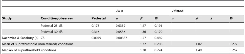
When Y_Weibull(Dx) is plotted on a log abscissa, changing the

value ofashifts the function horizontally, but otherwise leaves it

unchanged (Figure 2A), and changing the value of b linearly

stretches or compresses the function horizontally, leading to a change of slope (Figure 2B). On this log abscissa, the Weibull function always has the same basic shape, up to a linear horizontal

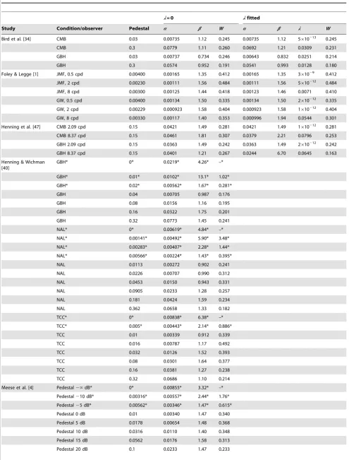
Table 1.Fitted Weibull function parameters for 2AFC contrast discrimination.

l= 0 lfitted

Study Condition/observer Pedestal a b W a b l W

Bird et al. [34] CMB 0.03 0.00735 1.12 0.245 0.00735 1.12 5610213 0.245

CMB 0.3 0.0779 1.11 0.260 0.0692 1.21 0.0309 0.231

GBH 0.03 0.00737 0.734 0.246 0.00643 0.832 0.0251 0.214 GBH 0.3 0.0574 0.952 0.191 0.0541 0.993 0.0128 0.180 Foley & Legge [1] JMF, 0.5 cpd 0.00400 0.00165 1.35 0.412 0.00165 1.35 361029 0.412

JMF, 2 cpd 0.00230 0.00111 1.56 0.484 0.00111 1.56 5610212 0.484 JMF, 8 cpd 0.00300 0.00125 1.44 0.418 0.00123 1.46 0.0071 0.410 GW, 0.5 cpd 0.00400 0.00134 1.50 0.335 0.00134 1.50 2610212 0.335 GW, 2 cpd 0.00229 0.000923 1.58 0.404 0.000923 1.58 1610212

0.404 GW, 8 cpd 0.00330 0.00117 1.40 0.353 0.000996 1.94 0.0544 0.301 Henning et al. [47] CMB 2.09 cpd 0.15 0.0421 1.49 0.281 0.0421 1.49 1610212

0.281 CMB 8.37 cpd 0.15 0.0461 1.81 0.307 0.0379 2.21 0.0796 0.253 GBH 2.09 cpd 0.15 0.0363 1.49 0.242 0.0363 1.49 2610212

0.242 GBH 8.37 cpd 0.15 0.0401 1.21 0.267 0.0244 6.70 0.0645 0.163 Henning & Wichman

[40]

GBH* 0* 0.0219* 4.26* –*

GBH* 0.01* 0.0102* 13.1* 1.02*

GBH* 0.02* 0.00562* 1.67* 0.281*

GBH 0.04 0.00705 0.987 0.176

GBH 0.08 0.0156 1.16 0.195

GBH 0.16 0.0322 1.75 0.201

GBH 0.32 0.0773 1.45 0.241

NAL* 0* 0.00619* 4.84* –*

NAL* 0.00141* 0.00492* 5.90* 3.48* NAL* 0.00283* 0.00407* 2.28* 1.44* NAL* 0.00566* 0.00224* 1.43* 0.395*

NAL 0.0113 0.00272 0.902 0.241

NAL 0.0226 0.00707 0.990 0.312

NAL 0.0453 0.0150 0.943 0.331

NAL 0.0905 0.0233 1.28 0.257

NAL 0.181 0.0424 1.59 0.234

NAL 0.362 0.0658 1.33 0.182

TCC* 0* 0.00838* 6.38* –*

TCC* 0.005* 0.00443* 2.14* 0.886*

TCC 0.01 0.00339 0.912 0.339

TCC 0.016 0.00787 1.17 0.492

TCC 0.032 0.0126 1.52 0.393

TCC 0.08 0.0301 1.64 0.377

TCC 0.16 0.0381 1.27 0.238

TCC 0.32 0.0686 1.10 0.214

changing the value of a linearly stretches or compresses the function horizontally as well as changing the threshold (Figure 2C),

while changing the value ofbchanges the shape of the function in

a way that cannot be described as a linear horizontal scaling (Figure 2D).

Sincebis proportional to the slope of the Weibull function on a

log abscissa, the low value of b for contrast discrimination

(compared with detection) often leads to the psychometric function for discrimination being described as ‘‘shallow’’, and that for

detection as ‘‘steep’’. However, psychometric functions for contrast

discrimination can besteeperthan for detection when plotted on a

linearcontrast abscissa (e.g., Nachmias & Sansbury [6], Figure 2; Foley & Legge [1], Figure 1). We must therefore be vigilant not to

be misled by the common practice of referring tobas the ‘‘slope’’

parameter.bdoes control the slope of the Weibull function on a

log abscissa, and this fact plays a key role in the proof of Theorem 2 of this paper, but the psychometric function is often plotted on a

linear abscissa, and, in this case,a and b both affect the slope

(Figures 2C and 2D); on a linear abscissa,aadditionally controls

the threshold andbadditionally controls the overall shape of the

psychometric function. Thus, when considering a linear abscissa, it

would be more appropriate to describe b as the ‘‘shape’’

parameter, rather than the ‘‘slope’’ parameter.

The Weibull function defined in Equation (1) asymptotes to

perfect performance (PWeibull~1). This is rarely achieved by

human observers due to lapses of concentration, etc., and this can

lead to a dramatic underestimation ofbif the observer makes just

one lapse on an easy trial [7]. Because of this problem, many researchers use a version of the Weibull function that includes a

‘‘lapse rate’’ parameter,l:

PWeibull~(1{l){(0:5{l) exp{(Dx=a)b

: ð2Þ

This function asymptotes toPWeibull~(1{l), and reduces to

Equation (1) in the case of l~0. The psychometric function

described by Equation (2) would result if the observer performed

according to Equation (1) on a proportion(1{2l) of trials, and

guessed randomly on the remaining trials.

The Weibull function was originally proposed by Weibull [8] as a useful, general-purpose statistical distribution. Its widespread use as a psychometric function can be traced back to Quick [9], who was apparently unaware of Weibull’s prior work. Quick proposed this function because, given certain assumptions, the Weibull function makes it easy to calculate how detection performance will be affected by adding extra stimulus components, or increasing the size or duration of the stimulus, an approach that has become Table 1.Cont.

l= 0 lfitted

Study Condition/observer Pedestal a b W a b l W

Pedestal 25 dB 0.178 0.0339 1.47 0.191 Pedestal 30 dB 0.316 0.0536 1.36 0.170 Nachmias & Sansbury [6] CS 0.0079 0.00387 1.27 0.489

Mean of suprathreshold (non-starred) conditions 1.32 0.298 1.82 0.297

Median of suprathreshold conditions 1.38 0.274 1.49 0.267

This table shows Weibull parameters fitted to 2AFC contrast discrimination data from six studies. The data from Meese et al. [4] are for their Binocular condition (plotted as squares in their Figure 5); these data were kindly provided by Tim Meese. For the other five papers, we read off the data points from digital scans of the figures (Bird et al. [34], Figure 1; Foley and Legge [1], Figure 1; Henning et al. [47], Figure 4 (sine wave stimuli only); Henning & Wichmann [40], Figure 4; Nachmias & Sansbury [6], Figure 2). In most cases, these figures plotted the proportion correct,P, for several different contrast differences,Dc, and we fitted the Weibull function using a maximum-likelihood method; specifically, we fitted the Weibull function by maximizing the expressionP_DcPlog½YWeibull(Dc)z½1{Plog½1{YWeibull(Dc), where YWeibullis the Weibull function whose parameters were being fitted. In Henning & Wichmann’s [40] paper, the figures plotted theDcvalues corresponding to 60%, 75%, and 90% correct on thefitted psychometric functions, so we had to fit Weibull functions to points sampled from Henning & Wichmann’s own fitted psychometric functions, rather than to the raw data. Where possible, we fitted both the lapse-free Weibull function of Equation (1), and the Weibull function of Equation (2), which includes a fitted lapse rate parameter,l. Parameters for the former fit appear under the heading ‘‘l~099, and those for the latter appear under the heading ‘‘lfitted’’. In many cases, the data did not sufficiently constrainlbecause there were no data points on the saturating portion of the psychometric function; in addition, Meese et al. ’s Weibull fits did not include a lapse rate parameter. The Weber fraction,W, is given byaxp, wherexpis the pedestal value. The means and medians at the bottom of the table are calculated from those studies for which the pedestal level exceeds the detection threshold, so that both stimuli were clearly visible. The cases where the pedestal is below detection threshold are stared in the table, and these were excluded from the means and medians.

doi:10.1371/journal.pone.0074815.t001

0.8 1 1.2 1.4 1.6 1.8 2 2.2 2.4 0

2 4 6 8 10 12 14 16

Number of conditions

Fitted Weibull β

Figure 1. Distribution of fitted Weibullbvalues in Table 1.The

known as probability summation[10–13]. Quick focused on yes/no detection tasks, where the observer has to make a binary decision about a single stimulus (as opposed to the 2AFC tasks that we consider in this paper, in which the observer makes a binary decision about a pair of stimuli), but a similar analysis can be applied to 2AFC tasks [2].

Most treatments of probability summation with the Weibull function invoke the ‘‘high threshold assumption’’ that a zero-contrast stimulus never elicits a response in the detection mechanism, so detection errors are always unlucky guesses. This assumption makes a number of predictions that have turned out to be false [2,14–16]. Furthermore, the convenient mathematics of probability summation with the Weibull function only applies to

detection. For suprathreshold discrimination, where both stimuli are easily detectable, these computational benefits do not apply. Despite this, many researchers have continued to use the Weibull function to fit data from both detection and discrimination experiments for three perfectly valid reasons: it is well-known, fits well to the data, and is built into QUEST [17], probably the most widely used adaptive psychophysical method.

Different models of visual processing will deliver different mathematical forms for the psychometric function. Therefore, because of the widespread practice of fitting a Weibull function to data, it is of interest to know what happens when we fit a Weibull function to a psychometric function that is not a Weibull. In Theorem 2 of this paper, we derive a general analytical expression

that gives a very accurate approximation ofbwhen the Weibull

function is fitted to non-Weibull psychometric functions. Although the usage of the Weibull function has its origin in outdated theoretical views, the Weibull function has very recently become more relevant again, due to the work of Neri [18]. He argues that the internal noise on the decision variable has a Laplace distribution, which, as we explain later in this

Introduction, can lead to a psychometric function that has the

form of a Weibull function withb~1.

First, we consider how the psychometric function might arise from the properties of the observer. In 2AFC discrimination experiments, the observer can be modelled using a transducer, followed by constant additive noise. The transducer converts the

stimulus value,x, into some internal scalar signal value,R(x).Ris

called the transducer function. A noise sample from a stationary,

stimulus-invariant distribution is then added to the internal signal, R(x), to give a noisy internal signal value. If the noise has zero

mean, thenR(x)will be the mean internal signal for stimulus value

x. The observer compares the noisy internal signal values from the

two stimuli, and chooses the stimulus that gave the higher value. From the experimenter’s perspective, the observer behaves as if

a sample of noise,e, is added to the difference of mean signals,z,

given by

z~h(Dx)~R(xpzDx){R(xp): ð3Þ

The observer is correct whenzzew0, i.e. whenew{z. The

probability,P, of this happening is given by

P~ Ð

?

{z

f(e)de, ð4Þ

wherefis the probability density function (PDF) of the noise, e.

This integral corresponds to the shaded area in Figure 3A.fhas to

be even-symmetric, even if the noise added to the output of the

transducer is not. This is because the noise sample onzis equal to

the noise sample on the target minus the noise sample on the nontarget. This is equivalent to swapping the sign of the nontarget

0.25 0.5 1 2 4 8 16 32

0.5 0.6 0.7 0.8 0.9 1

α = 1, β = 2 α = 2, β = 2 α = 4, β = 2

0.25 0.5 1 2 4 8 16 32

0.5 0.6 0.7 0.8 0.9 1

α = 2, β = 1 α = 2, β = 2 α = 2, β = 4

0 2 4 6 8

α = 1, β = 2 α = 2, β = 2 α = 4, β = 2

0 2 4 6 8

α = 2, β = 1 α = 2, β = 2 α = 2, β = 4 A

B

C

D

Δx

Proportion correct

Figure 2. Effect of varying Weibullaandbon log and linear abscissas.(A) Varyingaon a log abscissa: The curve shifts horizontally. (B) Varyingb

noise sample and adding it to the target noise sample. The sign-reversed noise sample on the nontarget will have a PDF with mirror symmetry relative to the PDF of the noise sample on the target, so the sum of these two values will have an even-symmetric

PDF. From the even symmetry offwe have

P~F(z)~ Ð z

{?

f(e)de, ð5Þ

where F is the cumulative distribution function (CDF) of the

observer’s noise on the internal difference signal, and corresponds to the shaded area in Figure 3B. So the psychometric function for

2AFC discrimination, expressed as a function ofz, will trace out

the positive half of the internal noise CDF, increasing from 0.5 to 1

aszincreases from 0 to‘.

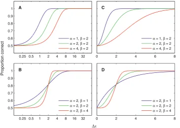
Figure 4 plots the CDFs and PDFs for several different forms of noise distribution (the mathematical definitions of these

distribu-tions will be given later). These CDFs (plotted as funcdistribu-tions ofz) do

not have a sigmoidal shape: The point of inflection is at zero on the abscissa. This is because the point of inflection corresponds to the peak of the derivative, and the derivative of these functions is the noise PDF, which peaks at 0 in each case.

In summary,Fis the CDF of the internal noise, and takes an

input ofz(Equation (5)); zis the output of h, a function that is

determined by the transducer and pedestal, and takes an input of

Dx(Equation (3)). The composition of these two functions, F0h,

gives the observer’s psychometric function when it is plotted as a

function of Dx. We use Y to represent this composition of

functions:

P~Y Dð xÞ

~ðF0hÞðDxÞ

~F h½ ðDxÞ

~F zð Þ

~F R x pzDx{R xp :

ð6Þ

f(ε)

−z 0

Noise, ε

A

f(ε)

z

0

Noise, ε

B

Figure 3. Graphical representation of the probability of a

correct response.The shaded areas in A and B correspond to the

integrals in Equations (4) and (5), respectively. The smooth curves trace out the PDF of the noise,f(e) on the internal difference signal,z. As explained in the text,fhas to be even-symmetric, and this means that the two integrals in Equations (4) and (5) are equal. The shaded areas correspond to the probability of a correct response. The psychometric function (expressed as a function of z) is the CDF of the noise, increasing from 0.5 to 1 aszincreases from 0 to‘.

doi:10.1371/journal.pone.0074815.g003

0.5 0.6 0.7 0.8 0.9 1

F

(

z

)

A

0 0.1 0.2 0.3 0.4 0.5 0.6

z

f

(

z

)

E

B

z F

C

z G

D

z H

Figure 4. CDFs and PDFs of four different noise distributions.The top row shows noise CDFs,F(z), for (A) a Laplace distribution (generalized

Gaussian withr~1), (B) a Gaussian distribution (generalized Gaussian withr~2), (C) a generalized Gaussian withr~4, (D) a logistic distribution. Each panel in the bottom row shows the PDF,f(z), corresponding to the CDF above it. Only the positive halves of the distributions are shown (i.e.

If we fit the Weibull function,Y_Weibull, of Equation (1) to the

psychometric function,Y, of Equation (6), then the Weibull slope

parameter,b, will be determined by both the noise CDF,F, and

the transducer, R. In Theorem 2, we show that, to a good

approximation,bcan be partitioned into a product of two factors,

bNoise and bTransducer. bNoise estimates the b of the Weibull

function that fits best to the noise CDF, whilebTransducerdepends

on the transducer function. Weibull b is found by multiplying

these two factors together. We derive general analytical formulae for both factors, and then derive, from these formulae, specific

expressions for bNoise for a variety of noise distributions, and

specific expressions for bTransducer for several commonly used

transducer functions.

Our work greatly extends a result previously published by Pelli [19]. He showed that, for 2AFC detection or discrimination,

b&bNoise|b: ð7Þ

where bis the slope ofd’[20] against Dx on log-log axes. Pelli

derived this relationship using the concrete example of contrast

detection, but it is a purely mathematical relationship (outlined in his ‘‘Analysis’’ section, Ref. [19], p. 121), which makes no assumptions about the underlying model, and could equally well be applied to

discriminationalong any unspecified stimulus dimension by

replac-ing the contrast term,c, withDxin his Equations (14) to (21).

Pelli’s analysis ran as follows. Given thedefinitionofd’for 2AFC,

d’~pffiffiffi2W{1_{(P) ð8Þ}

(where W is the cumulative Gaussian), and the observation or

assumption d’~ðDx=Dx0:76Þb (where Dx0:76 is the value of Dx

corresponding to a proportion correct ofW(1 ffiffiffip2)&0:76, giving

d’~1, andbis the log-log slope ofd’againstDx), we have

P~W Dð x=Dx0:76Þb . ffiffiffi

2

p

h i

: ð9Þ

Note that Equation (9) has the same form as Equation (6) if the

pedestal,xp, is zero, the transducer is a power function,R(x)!xb,

and the internal noise CDF is the cumulative Gaussian (as is

usually assumed). If we letbNoise represent theb of the Weibull

function, Y_Weibull(:), that fits best to the cumulative Gaussian,

W(:), then, substituting this Weibull function forW(:)in Equation

(9) yields a Weibull function withbgiven bybNoise|b, which is

Relation (7).

In our terms, the ‘‘b’’ part of Relation (7) isbTransducer, the factor

determined by the transducer; we will show that, in the case of a power-function transducer and zero pedestal, our general

expres-sion for bTransducer reduces to b. We obtain Weibull b by

multiplying bNoise and bTransducer together, resulting in an

estimated bgiven bybEst~bNoise|bTransducer, which is equal to

bNoise|bin the scenario just described. In this paper, we derive

general analytical expressions forbNoiseandbTransducerso that we

can easily estimate Weibull b for any combination of noise

distribution and transducer function, not just the specific case considered by Pelli.

In many situations, the observer can be modelled using a linear

filter. This is equivalent to using a linear transducer,R(x)~rx,

whereris a constant. For this transducer, Equation (6) gives

Y(Dx)~F(rDx) for a linear transducer,R xð Þ~rx: ð10Þ

Thus, the linear observer’s psychometric function (plotted on a

linear abscissa,Dx) will have the same basic shape as the internal

noise CDF,F, just differing by a horizontal scaling factor,r. So, if

the observer behaves in a linear fashion, the psychometric function plotted on linear axes gives us a direct plot of the shape of the

internal noise CDF. In this situation, sincebcontrols the Weibull

function’s shape on linear axes, the b that fits best to the

psychometric function will be thebthat fits best to the noise CDF

(the sensitivity parameter,r, will determine the best-fittinga, since

acontrols the Weibull function’s horizontal scaling on linear axes).

The internal noise is usually assumed to be Gaussian, but Neri [18] has recently disputed this assumption. Using reverse correlation methods, he attempted to measure both the ‘‘deter-ministic transformation’’ (in our terms, the transducer function for contrast), and the shape of the internal noise distribution. He concluded that, for temporal 2AFC detection of a bright bar in noise, the contrast transducer was linear, and the internal noise had a Laplace distribution (whose CDF and PDF are given in Figures 4A and 4E, respectively). This is a radical departure from the Gaussian assumption that has usually been made since the invention of signal detection theory in the 1950s [14]. The Laplace distribution has higher kurtosis (i.e., has a sharper peak and heavier tails) than the Gaussian (compare Figure 4E with 4F). As

we shall see later on, for positivez, the Laplace distribution has a

CDF that takes the form of a Weibull function withb~1. Since

the psychometric function has the same shape as the internal noise CDF for a linear observer, Neri’s proposal that the transducer is linear and the internal noise has a stimulus-independent Laplace distribution predicts that the observer’s psychometric function

should, like the Laplace CDF, be a Weibull function withb~1. As

noted earlier (and shown in Table 1 and Figure 1), this does not

generally seem to be the case – with noise-free stimuli,bis around

3 for contrast detection and, even for suprathreshold contrast

discrimination, where b is substantially lower, it is still usually

found to be greater than 1; later, we shall show that, assuming

additive noise, these b values are more consistent with a

distribution that haslowerkurtosis than a Gaussian.

Although the whole of this paper is couched in terms of the transducer model, it is not necessary to accept the transducer model to find the results useful; we just have to assume that the

psychometric function has a form consistent with a particular

combination of internal noise distribution and transducer function. For example, the intrinsic uncertainty model produces

psycho-metric functions that areconsistentwith additive noise following an

expansive power-function transducer with exponent that increases with channel uncertainty [21], but the model itself has no explicit transducer. Alternatively, suppose the observer carries out the discrimination task by making noisy estimates of each stimulus value and comparing them. Due to the noise, repeated

presen-tations of the same stimulus value,x, will give a distribution of

estimated values,^xx, around the mean estimate. If we can find a

function,R, such that the shape and width of the distribution of

R(^xx) is independent of x, then the observer is equivalent to a

transducer model with additive noise. In this class of model, the

stimulus value,x, is transduced to giveR(x), and then

In keeping with our terminology of Ph for the threshold

performance level, we introduce the termszhandDxhto represent

the values ofzandDxat threshold, i.e. the values ofzandDxwhen

the proportion correct isPh, which we define as1{0:5=e.

Theorum 1. A General Expression for the

Psychometric Function in Terms of the Stimulus Values and the Threshold

Introduction

Equation (6) gives a general equation for the psychometric

function in terms of the transducer function, R, and the noise

CDF, F. The sensitivity of the system (which determines the

discrimination threshold,Dxh) can be adjusted either by changing

the gain of the transducer function (i.e., stretching or compressing

R along its vertical axis), or by adjusting the spread of the noise

CDF (i.e., stretching or compressingFalong its horizontal axis), or

both. Since the units in which we express the internal signal are arbitrary, researchers will usually either (1) fix the spread of the noise CDF at some convenient standard value (say, unit variance), and vary the transducer gain to achieve the desired threshold, or (2) fix the gain of the transducer at some convenient standard value (say, unit gain), and vary the spread of the noise CDF to achieve the desired threshold. However, for our purposes, it is more

convenient to reformulate Equation (6) so thatboththe spread of

the noise CDFandthe gain of the transducer are set to convenient

values, and the threshold is specified directly. This allows us to consider general forms of the transducer and noise, without having to worry about specifying the gain of the transducer or spread of the noise correctly – the reformulated equation will take care of the spread of the psychometric function automatically. Theorem 1 derives an expression for the psychometric function that meets these requirements.

Statement of Theorem 1 Theorem 1 has three parts:

1. The expression for the psychometric function, Y(Dx), in

Equation (6) can be rewritten as.

Y Dð xÞ~F F{1ðPhÞ

R x pzDx{R xp R xpzDxh

{R xp

! , ð11Þ

where Dxh is the stimulus difference corresponding to a

performance level ofPh.

2. If we change the gain of the transducer by replacing the

function R(x) with rR(x), this will have no effect on the

psychometric function,Y(Dx)in Equation (11).

3. Similarly, if we change the spread of the noise CDF by

replacing the functionF(z)withF(z=s), this will have no effect

onY(Dx)in Equation (11).

Proof of Theorem 1

First, let us substitute the threshold values of P and Dx into

Equation (6):

Ph~F R xpzDxh

{R xp

: ð12Þ

Equation (12) can be rearranged to give

F{1 _P h

ð Þ

R x pzDxh{R xp

~1: ð13Þ

Since the left hand side of Equation (13) is equal to 1, we can multiply anything by this expression, and leave it unchanged.

Multiplying the argument ofFin (6) by this expression, we obtain

Equation (11), which proves Part 1 of the theorem. If we replace

the transducer,R(x), in Equation (11) with one that has a different

gain, rR(x), the r’s will obviously cancel out, leaving the

psychometric function, Y, unchanged, which proves Part 2 of

the theorem. To prove Part 3 of the theorem, consider what

happens if we replace the function,F(z), in Equation (11) with one

that has a different spread,F(z=s). Then the inverse function is

given bysF{1_{(P), and thes’s cancel out:}

YðDxÞ~F

sF{1_P h

ð ÞR xpzDx

{R xp

R x pzDxh{R xp s

0 B B B @

1 C C C A

~F F{1ðPhÞ

R xpzDx

{R xp

R x pzDxh{R xp

! ,

which is identical to Equation (11).%

Discussion of Theorem 1

Equation (11) gives us an expression for the psychometric

function (parameterized by the threshold,Dxh) in which we can

use any convenient standard form of the transducer function or noise distribution, without having to worry about setting the right gain or spread.

Although, for most of this paper, we define the threshold as the

stimulus difference that gives rise to a performance level, Ph,

defined as1{0:5=e, Theorem 1 actually holds for any value that

Phcould have taken.

Note that, in the special case of a zero pedestal (xp~0) and a

transducer that gives zero output for zero input (R(0)~0),

Equation (11) reduces to

Y Dð xÞ~F F{1ðPhÞ RðDxÞ

RðDxhÞ

if xp~0and R(0)~0: ð14Þ

Theorem 2: An Expression That Estimates the Best-Fitting Weibull

b

Statement of Theorem 2 Theorem 2 has two parts:

1. If the parameters of the Weibull function, YWeibull(Dx), of

Equation (1) can be set to provide a good fit to Equation (6), then the best-fitting beta will be well approximated by

where bNoise and bTransducer are given by the following expressions:

bNoise~2eF{1_P h

ð Þf F{1_P h

ð Þ

, ð16Þ

bTransducer~ R’ xpzDxh

Dxh R x pzDxh{R xp

, (17)and f and R’ are the

derivatives of, respectively,FandRwith respect to their inputs.

2. bNoiseis an estimate of theb of the Weibull function that fits

best to the noise CDF,F, in Equation (6).

Proof of Theorem 2

By assumption, the Weibull function provides a close fit toYof

Equation (6), so the gradient ofYat threshold will closely match

the gradient of the best-fitting Weibull function at threshold.

Therefore, sinceb is proportional to the gradient of the Weibull

function at threshold with an abscissa oflog (Dx), we can derive a

close approximation tobfrom the gradient ofYat threshold on

this abscissa. To create a log abscissa, lety~ln (Dx), so that

Dx~ey: ð18Þ

If we substitute ey _{for Dx in Equation (1), we find that the}

gradient of the Weibull function on the log abscissa,y, is given by

dPWeibull dy ~

b 2

Dx a

b

exp { Dx a

b

" #

: ð19Þ

For the Weibull function at threshold performance

(PWeibull~Ph), it follows that Dx~a. Substituting a for Dx in (19) gives

dPWeibull dy

_P

Weibull~Ph ~b

2e, ð20Þ

and so

b~2edPWeibull dy

_P

Weibull~Ph

: ð21Þ

To evaluate Equation (21), we use the chain rule to expand the derivative:

b~2edPWeibull dz |

dz dy _P

Weibull~Ph

: ð22Þ

As noted above, the assumed good fit of the Weibull function,

YWeibull, of Equation (1) to Y of Equation (6) means that the

output,PWeibull, of the Weibull function is close to the output ofY,

which is the proportion correct,P. Substituting Pfor PWeibull in

Equation (22) therefore gives us a good estimate ofb, which we

callbEst:

bEst~2edP dz|

dz dy _P~P

h

: ð23Þ

From Equation (6), we see thatP~F(z), sodP=dzis given by

f(z), the noise PDF (which is the derivative ofF(z)with respect to

z). At threshold,z~zh, and so,

bEst~2ef(zh)| dz dy

P~P_h

: ð24Þ

We will see that the first part of Equation (24), 2ef(zh), is

proportional tobNoise, theb-estimate of the Weibull function that

fits best to the noise CDF, and the second part,dz=dyat threshold,

is proportional to bTransducer defined above. Most of the work

involves deriving an expression fordz=dyat threshold.

Using Equation (18) to substitute forDxin Equation (3), we get

z~R x pzey{R xp : ð25Þ

Let us definext as the target stimulus value:

xt~xpzDx~xpzey: ð26Þ

Using Equation (26) to substitute forxpzey in Equation (25),

we have

z~R xð Þt {R xp : ð27Þ

Then,

dz dy~

dz dxt

|dxt dy

~R0ð Þxt ey

~R0 xpzDx

Dx,

ð28Þ

where R’ is the derivative of R with respect to its input. At

threshold, we can substituteDxhforDxin Equation (28), giving

dz dy

P~P_h

~R0 xpzDxh

Dxh: ð29Þ

Using Equation (29) to substitute fordz=dyin Equation (24), we

obtain

bEst~2ef(zh)R’ xpzDxh

Dxh: ð30Þ

From Equation (6), we haveP~F(z), so, considering the values

zh~F{1ðPhÞ: ð31Þ

Using Equation (31) to substitute forzh in Equation (30), we

have

bEst~2ef F{1_P h

ð Þ

R’xpzDxh

Dxh: ð32Þ

To evaluate this expression as written in Equation (32), we need to know the gain of the transducer and the spread of the noise CDF, or at least their ratio. However, if we know the shape of the transducer (apart from the gain), and we know the shape of the noise CDF (apart from the spread), we can work out the ratio of

gain to spread from Dxh. But it is much more convenient to

reformulate Equation (32) so that this is taken care of, and we can arbitrarily set the spread of the noise CDF and the gain of the transducer to any convenient values. We can use the same trick that we used in Theorem 1: We multiply the expression in Equation (32) by the left hand side of Equation (13), which equals 1. After doing this, and rearranging the terms, we obtain

bEst~2eF{1_P h

ð Þf F{1_P h

ð Þ

| R’ xpzDxh

Dxh R xpzDxh

{R xp

: ð33Þ

Equation (33) can be written in the form given by Equations (15) to (17), which proves the Part 1 of the theorem.

We now prove Part 2, that bNoise is the estimated b of the

Weibull function that fits best to the noise CDF,F. First, note that

all linear transducers have the form R(x)~rx. This gives

R’(x)~r, and so, from Equation (17), bTransducer~1, regardless

of the value ofr,xporDxh. Therefore, from (15),bEst~bNoisefor

a linear transducer. Now, consider the linear transducerR(x)~x.

For this transducer, Equation (6) gives Y(Dx)~F(Dx). The

estimate ofbwhen the Weibull function,YWeibull(Dx), is fitted to

Y(Dx) is given by bEst~bNoise, as it will be for any linear

transducer. Since, in this case, Y(Dx)~F(Dx), the Weibull

function has also been fitted to the noise CDF, and the estimatedb

of this fitted function is given bybEst~bNoise.%

Discussion of Theorem 2

To get an intuition into how Weibullbis partitioned into the

two terms,bNoiseandbTransducer, let us refer back to Equation (21).

This equation shows that b is proportional to dPWeibull=dy at

threshold. We used the chain rule to express dPWeibull=dy as

dPWeibull=dz|dz=dy, which is approximately equal to f(zh)|dz=dy. f(zh) depends only on the noise distribution, and

is proportional tobNoise;dz=dyat threshold generally depends on

the transducer, the pedestal and the threshold, and is proportional tobTransducer; their product is proportional to Weibullb. This is essentially where Equations (15) to (17) come from. The equations were tidied up by specifying the constants of proportionality, and

defining bNoise and bTransducer in such a way that they are

independent of any horizontal scaling of the noise distribution, or

any vertical scaling of the transducer function. Thus, thebNoise

term will be the same for, for example, all Gaussian distributions,

whatever the spread, and thebTransducerterm will be the same for,

for example, all power functions with a particular exponent, whatever the gain.

Equation (17) expressesbTransduceras a function of the threshold

stimulus difference,Dxh. Alternatively, for nonzero pedestals, we

can reformulate Equation (17) as a function of the Weber fraction,

W, defined as the ratioDxxpat threshold:

W~Dxhxp: ð34Þ

From Equation (34), we obtain Dxh~Wxp, and, using this

expression to substitute forDxh in Equation (17), we can rewrite

the expression forbTransducerin terms ofW:

bTransducer~ R’ xpð1zWÞ

Wxp R xpð1zWÞ

{R xp

ifxp=0: ð35Þ

Δx_θ ΔR_θ

(x_p + Δx_θ, R(x_p + Δx_θ))

(x

p, R(xp))

A

Transducer output,

R

(

x

)

Transducer input, x

Δx_θ ΔR_θ

(x_p + Δx_θ, R(x_p + Δx_θ))

(x

p, R(xp))

B

Transducer input, x

Δx_θ ΔR_θ

(x_p + Δx_θ, R(x_p + Δx_θ))

(x

p, R(xp))

C

Transducer input, x

Figure 5. Geometrical interpretation of the expression forbTransducer_{.In each panel, the thick, magenta curve represents the transducer}

function. The horizontal axes represent the transducer input, and the vertical axes represent the transducer output.xpis the pedestal level, andDxhis the discrimination threshold. The gradient of the blue line,DRh=Dxh, is equal toV, defined in Equation (39). The green line is the tangent to the transducer at pointxpzDxh,R xp zDxh; its gradient is equal toU, defined in Equation (38). The ratioU=Vis equal tobTransducer. For an expansive transducer (panel A),UwV, sobTransducerw1. For a compressive transducer (panel B),UvV, sobTransducerv1. For a linear transducer (panel C),

U~V, sobTransducer_~1.

The Weber fraction can only be defined ifxp=0. Ifxp~0and R(0)~0, Equation (17) reduces to

bTransducer~R’ðDxhÞDxh RðDxhÞ

ifxp~0 andR(0)~0: ð36Þ

When the stimulus dimension of interest is contrast, a discrimination experiment with a zero pedestal is called a contrast detection experiment.

One important property ofbTransduceris that it is always greater

than 1 for a fully expansive transducer function (i.e., one for which the slope always increases away from zero with increasing input), and is always less than 1 for a fully compressive transducer function (i.e., one for which the slope always decreases towards zero with increasing input). Here we provide a geometrical argument (illustrated in Figure 5) to explain why this is the case.

First, note that we can rewrite Equation (17) as

bTransducer~U

V, ð37Þ

where

U~R’ xpzDxh

, ð38Þ

and

V~R xpzDxh

_{

R xp

Dxh

~DRh

Dxh

, ð39Þ

with

DRh~R x pzDxh{R xp : ð40Þ

These quantities are illustrated for an expansive transducer in Figure 5A, where the thick, magenta curve represents the

transducer. The filled circles mark points xp,R xp and

xpzDxh,R xpzDxh

. The gradient of the blue line connecting

these two points isV, defined in Equation (39). The short, green,

line segment is the tangent to the transducer at

xpzDxh,R x pzDxh

; its gradient is U, defined in Equation

(38). It is clear from the diagram that, for an expansive transducer, like the one illustrated, the gradient of the transducer at

xpzDxh,R xpzDxh

must always be steeper than the blue line, because, as we travel along the transducer function from

xp,R xp

to xpzDxh,R xpzDxh

, the transducer

approach-es the second point from below the blue line. Therefore,Umust

always be greater thanV, so, from Equation (37),bTransducermust

always be greater than 1.

Figure 5B illustrates the situation for a compressive transducer.

Here, as we travel along the transducer function fromxp,R xp

to xpzDxh,R xpzDxh

, the transducer approaches the second point from above the blue line, and so the gradient of the transducer at the second point must be lower than the gradient of

the blue line. Thus, U must always be less than V, so, from

Equation (37),bTransducermust always be less than 1.

Finally, Figure 5C illustrates the situation for a linear transducer, i.e. one that is neither expansive nor compressive. Here, the gradient of the transducer is equal to the gradient of the

blue line, soU~V, and thereforebTransducer~1. This provides a

geometrical insight into the previously proved fact that

bTransducer~1for a linear transducer.

In conclusion, Weibull b can be partitioned into two factors:

bNoise (Equation (16)), which estimates the b of the Weibull

function that fits best to the noise CDF, F; and bTransducer

(Equation (17), (35) or (36)), which is determined partly (or, as we shall see, sometimes completely) by the shape of the transducer

function, R. bTransducer is greater than 1 for an expansive

transducer, less than 1 for a compressive transducer, and equal

to 1 for a linear transducer.bNoiseis independent of the spread (i.e.

horizontal scaling) of the CDF (analogously, Weibull b is

independent of the spread of the Weibull function on linear axes); bTransducer is independent of the gain (i.e. vertical scaling) of the

transducer. Multiplying bNoise and bTransducer together gives us

bEst, the estimate of Weibull b. The expressions for bNoise and

bTransducerderived above are completely general. In later sections,

we derive values forbNoise given specific noise distributions, and

expressions forbTransducergiven specific transducers.

There are two possible sources of error in the Weibull b

estimate, bEst. Firstly, the derivation of the expression for bEst

relies on the use ofdP=dzas an approximation ofdPWeibull=dzat

threshold in the step from Equation (22) to (23), whereP is the

output of the psychometric function,Y, andPWeibullis the output

of the best-fitting Weibull function. The accuracy ofbEstrelies on

these two slopes being close at the threshold performance level. A second potential source of inaccuracy is that, even if these two slopes are very close at the threshold level, the overall

psycho-metric function,Y, might still not be well fit by a Weibull function,

in which case the best-fitting Weibullbcould deviate substantially

frombEst. However, as we will show, in the range of conditions

usually encountered, the Weibull function does provide a good fit

to the psychometric function, sobEstis accurate. In cases whereY

is a Weibull function, the best-fitting Weibull function will fit

exactly, andbEstgives the exact value of the best-fitting Weibullb.

DerivingbNoisefor Specific Noise Distributions

As proved in Theorem 2,bNoise is an estimate of thebof the

Weibull function that fits best to the noise CDF. In this section, we

evaluate the analytical expression for bNoise (Equation (16)) for

several different noise distributions. We also compare each value

with theb value obtained by fitting the Weibull function to the

noise CDF numerically. There is of course no single correct

answer to the question of what is the best-fittingb– it depends on

EvaluatingbNoisefor a generalized Gaussian noise CDF

Most psychophysical models use Gaussian noise. This is partly because the Gaussian is often easy to handle analytically, but also because, according to the Central Limit Theorem, the sum of independent sources of noise tends towards a Gaussian-distributed random variable, whatever the distribution of the individual noise sources. However, as noted earlier, Neri [18] has recently argued that internal sensory noise is closer to a Laplace distribution. Both the Gaussian and the Laplace are parameterizations of the generalized Gaussian, which we consider in this section.

The generalized Gaussian CDF is given by the following

expression, with horizontal scaling (i.e. spread) determined by t,

and shape determined byr:

P~F_Gen:Gaussian(z;r,t)~

1zsgn(z)c½ðDzD=tÞr;1=r

2 , ð41Þ

wheresgn(z)~1for z§0and {1for zv0, andcis the lower

incomplete gamma function, defined as

c fð ;nÞ~ 1

C(n) ðf

0

tn{1_e{t_{dt: ð42Þ}

C(n)in Equation (42) is the gamma function, which is a continuous

generalization of the factorial, given by

C(n)~Ð

?

0

tn{1_e{t_{dt: ð43Þ}

Note, the lower incomplete gamma function is often defined

without the normalization term,C(n), but it is more convenient for

us to define it as in Equation (42), because otherwise we would just

have to divide byC(n)anyway, complicating the expression for the

generalized Gaussian in Equation (41); in addition, the MATLAB function gammainc evaluates the function as defined in Equation (42).

The variance of the generalized Gaussian distribution is given by

sz2~

t2_Cð3=rÞ

Cð1=rÞ : ð44Þ

We use the subscript,z, in Equation (44) to indicate that this is

the variance of the noise on the difference of mean signals,z, as

opposed to the variance of the noise on the transducer outputs,

which we could call sR2. As long as the noise on the two

transducer outputs within a trial is uncorrelated and has zero

mean, then we havesz2~2sR2, and sosz~sR

ffiffiffi 2

p

, whatever form the noise CDF takes.

The PDF of the generalized Gaussian distribution is given by the derivative of the CDF:

fGen:Gaussian(z;r,t)~ r

2tCð1=rÞexp {

DzD

t

r

: ð45Þ

As noted above, the shape of the distribution is determined by

the parameter, r. When r~2, Equation (45) describes the

Gaussian PDF:

fGen:Gaussian(z;2,t)~ 1 sz

ffiffiffiffiffiffi 2p

p exp { z 2

2sz2

: ð46Þ

Whenr~1, Equation (45) describes the Laplace PDF:

fGen:Gaussian(z;1,t)~ 1 sz

ffiffiffi 2

p exp { DzD sz ffiffiffi2

p

!

: ð47Þ

For positive z, the inverse of the generalized Gaussian CDF is

given by

z~F{1

Gen:Gaussian(P;r,t)

~t c {1_ð2P{1;1=rÞ1=r ð48Þ

(we don’t need to worry about negative z, because, for any

monotonically increasing transducer, and positiveDx,zas defined

in Equation (3) is always positive). The inverse of the lower

incomplete gamma function, c{1_{, in Equation (48) can be}

evaluated using the MATLAB function gammaincinv. At thresh-old, P~Ph~1{0:5=e. Substituting these values into Equation (48), we get

F{1

Gen:GaussianðPh;r,tÞ~t c{1ð1{1=e;1=rÞ

1=r

: ð49Þ

We can use the expression forF{1

Gen:GaussianðPh;r,tÞin Equation

(49) to substitute forF{1_P

h

ð Þin Equation (16), and we can use the

expression forfGen:Gaussian(:;r,t)in Equation (45) to substitute for

f(:)in Equation (16). The different instances oftcancel out, giving

0 2 4 6 8

0 0.2 0.4 0.6 0.8 1 1.2 1.4 1.6 1.8 2

β

Noise

(

ρ

)

ρ

Figure 6.bNoise

Gen:Gaussianð Þr plotted as a function ofr.This curve plots

the predictedb when the Weibull function is fitted to the CDF of generalized Gaussian distributions with a range of differentrvalues. The graph asymptotes to a value ofe{1(see Appendix S1), indicated by the horizontal dashed line. The shape of the generalized Gaussian distribution is determined byr.r-values of 1 and 2 are special cases: r~1 gives a Laplace distribution, and r~2 gives a Gaussian distribution.

us an expression for bNoise for the generalized Gaussian noise

distribution that is a function ofr:

bNoise_Gen:Gaussianð Þr~ rI 1=r

Cð1=rÞexp 1ð {IÞ, ð50Þ

where

I~c{1_{ð1{1=e;1=rÞ: ð51Þ}

The subscript, ‘‘Gen.Gaussian’’, onbNoise_Gen:Gaussian in Equation (50)

indicates the general form of the noise CDF.

Figure 6 plotsbNoise_Gen:Gaussianð Þr as a function ofr. As proved in

Appendix S1, bNoise_Gen:Gaussianð Þr ?e{1 as r??. Values of

bNoise_Gen:Gaussianð Þr forr= 1, 2, and 4 are given by

bNoise_Gen:Gaussianð Þ1~1 ð52Þ

bNoise_Gen:Gaussianð Þ2~1:302 to 4 significant figuresð Þ ð53Þ

bNoise_Gen:Gaussianð Þ4~1:562 to 4 significant figuresð Þ: ð54Þ

The value ofbNoisefor the Laplace distribution (Equation (52)) is

exactly 1. This is because the positive half of its CDF is a Weibull

function with b~1. This can be seen from the fact that

c(f;1)~1{exp ({f), and so Equation (41) gives, for positivez,

FGen:Gaussian(z;1,t)~1{0:5 expð{z=tÞ: ð55Þ

The Weibull function withb~1therefore gives an exact fit to

the Laplacian noise CDF, and the estimated Weibullb, given by

bNoise~1, is exactly correct.

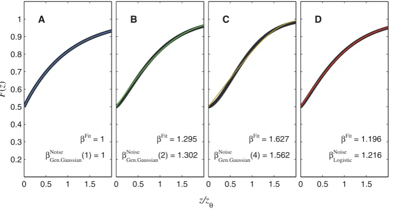
The coloured curves in Figures 7A, 7B, and 7C show the

generalized Gaussian noise CDFs forr= 1, 2, and 4, respectively,

and the thick, black curves show the best-fitting Weibull functions (maximum-likelihood fit over inputs from 0 to twice the threshold).

Also shown in each panel is the appropriate value ofbNoisefrom

equations (52) to (54), and the best-fitting Weibullb, which we call

bFit. As explained above, the match between bFit and bNoise is

exact for the Laplace (r~1, Figure 7A), but the match is also very

good for the other distributions. For the Gaussian (r~2,

Figure 7B), bFit~1:295, very close to our analytically derived

value of bNoise_Gen:Gaussianð Þ2~1:302. As discussed earlier, Pelli [19]

fitted the Weibull to a Gaussian CDF using a different fitting

0 0.5 1 1.5 0.2

0.3 0.4 0.5 0.6 0.7 0.8 0.9 1

F

(

z

)

βFit = 1

β_Gen.GaussianNoise (1) = 1

A

0 0.5 1 1.5

βFit = 1.295

β_Gen.GaussianNoise

(2) = 1.302

B

0 0.5 1 1.5

βFit = 1.627

β_Gen.GaussianNoise

(4) = 1.562

C

0 0.5 1 1.5

βFit = 1.196

β_LogisticNoise = 1.216

D

z/z

θ

Figure 7. Noise CDFs from Figure 4 plotted against the best-fitting Weibull functions.The thin, coloured curves shown in (A) to (D) are the

CDFs from Figures 4A to 4D, respectively. The thick, black curves are the Weibull functions that give the best (maximum-likelihood) fit across the range of inputs shown on the horizontal axis. This fit was carried out by maximizing the expression P_zF(z) log½YWeibull(z)z

½1{F(z)log½1{YWeibull(z), whereFis the noise CDF, and YWeibull is the Weibull function whose parameters were being fitted. The Weibull

function provides a perfect fit to the Laplace CDF (A), an excellent fit to the Gaussian (B), and logistic (D) CDFs, and an acceptable fit to the generalized Gaussian withr~4(C); this partly justifies our use ofPas an estimate ofPWeibullin Equation (23). ThebFitvalues are thebparameters of

the fitted Weibull functions. ThebNoisevalues are our analytical estimates ofbFit, given by Equations (52) to (54) for panels (A) to (C), respectively, and Equation (60) for panel (D). In each case,bNoiseprovides a close match tobFit. The parameter in brackets in eachbNoiseGen:Gaussian term is the shape

parameter,r(see Equation (50)). As noted in the text, the CDFs all have a point of inflection at zero. With the exception of panel A, the best-fitting Weibull functions have a point of inflection slightly above zero (bwould have to be 1 or less for the steepest point to occur at zero). Nevertheless, the Weibull functions still provide good fits.

method: He minimized the maximum error over all positive

inputs. Thebvalue he obtained from this fit was 1.247. As noted

earlier, there is no single ‘‘correct’’ answer, but our maximum-likelihood fitting paradigm is probably more representative of the process of fitting a function to psychophysical data, and our

obtainedbof 1.295 is very close to the analytically obtained value.

The match between bNoise and bFit forr~4(Figure 7C) is also

close, the deviation being far smaller than the margin of error

usually encountered when measuring Weibullb[22–27].

EvaluatingbNoisefor the logistic noise CDF

Sometimes, the logistic function is used instead of the Gaussian, for computational convenience (e.g. Ref. [28]). The logistic function is very similar in shape to the Gaussian. Its CDF is given by

P~FLogisticðz;tÞ~ 1

1zexp ({z=t): ð56Þ

As noted by Strasburger [29], this function is identical to the

hyperbolic tangent function, given by Ftanh(z;t)~0:5

ftanh½z=(2t)z1g. Its variance ist2_p2_{3. The PDF of the logistic}

distribution is given by the derivative of the CDF:

f_Logisticðz;tÞ~ exp ({z=t)

t½1zexp ({z=t)2: ð57Þ

The inverse of the logistic CDF is given by

z~F{1

LogisticðP;tÞ~{tln 1=Pð {1Þ, ð58Þ

At threshold,P~Ph~1{0:5=e. Substituting these values into

Equation (58), we get

F{1

LogisticðPh;tÞ~tln 2eð {1Þ: ð59Þ

We can use the expression forF{1

LogisticðPh;tÞin Equation (59) to

substitute for F{1 _P

h

ð Þ in Equation (16), and we can use the

expression forfLogistic(:) in Equation (57) to substitute forf(:)in

Equation (16). This gives

bNoise_Logistic~ln 2eð {1Þ½1{1=(2e)

~1:216 to 4significant figuresð Þ:

ð60Þ

As before, the subscript onbNoise indicates the form of noise

CDF. The accuracy of this approximation is confirmed in

Figure 7D. The b parameter of the fitted Weibull function

(bFit~1:196) is very close to the estimated value from Equation (60).

Theorem 3. Tendency towards Linear Behaviour with Non-Zero Pedestals

Introduction

As shown earlier, for a linear transducer,bTransducer~1, and so

bEst~bNoise, which takes a value of around 1.3 for Gaussian

internal noise. So, if a transducer model has additive Gaussian

noise and generates psychometric functions with a Weibullb of

about 1.3, that might seem to suggest that it contains a linear transducer. However, a transducer model with additive Gaussian

noise can in fact generate psychometric functions withb&1:3for

suprathreshold contrast discrimination even when the transducer departs wildly from a linear function [4]. Theorem 3 explains how this occurs.

Statement of Theorem 3

If the gradient of the transducer is not 0 or‘at the pedestal

level, then, asDxh?0,bTransducer?1.

Proof of Theorem 3

As noted earlier,bTransducer~U=V, whereUandVare given in

Equations (38) and (39), respectively. The limit ofVasDxh?0is

the derivative ofRatxp, i.e.R’ xp , by definition of the derivative,

and the limit ofUasDxh?0is obviouslyR’ xp , so we have

lim Dx_h?0U

~ lim Dx_h?0V

~R’ xp : ð61Þ

Then, provided thatR’ xp is not 0 or‘, we have

lim Dx_h?0b

Transducer_{~ lim} Dx_h?0

U V~

lim Dx_h?0U

lim Dx_h?0V

~R’ xp R’ xp

~1: ð62Þ

If R’ xp is 0 or ‘, then R’ xp R’ xp is an indeterminate

form, 0=0 or?=?, and cannot be evaluated. In this case, we

cannot evaluate the limit ofbTransducerby dividing the limit ofUby

the limit ofV. The limit must instead be evaluated in some other

way that will depend on the form of the transducer, and the limit in this case will not necessarily be 1.

Discussion of Theorem 3

Theorem 3 shows that,whateverthe transducer function, as long

as its gradient is not 0 or‘at the pedestal level, Weibullbwill

approach that for a linear transducer as sensitivity improves. Virtually all proposed transducers do have a finite, nonzero gradient for nonzero inputs; therefore, if the internal noise is

approximately Gaussian, we would expect Weibullbto be close to

1.3 for suprathreshold contrast discrimination. Detection and discrimination data are often fitted with a power-function transducer or a Legge-Foley transducer (both considered below),

and, with these transducers, the gradient is 0 or‘at an input level

of zero. Thus, for these transducers, when the pedestal level is

zero, Equation (62) does not apply, andb does not necessarily

approach that for a linear transducer as sensitivity improves. This explains why, for contrast detection experiments (i.e. when the

pedestal is zero), Weibullbhas been found to deviate greatly from

the value of 1.3 expected from a linear transducer with Gaussian noise.

Consider what happens in general when the pedestal

approach-es zero. If we assume thatR(0)~0, then, asxpdrops belowDxh,

bothU(Equation (38)) andV(Equation (39)) become dominated

by theDxh term, and bTransducer approaches the value given in

Equation (36), which is not, in general, equal to 1. Thus, we would

low pedestals. Meese, Georgeson and Baker [4] showed that this is indeed the case for visual contrast discrimination, and we examine their work in more detail later, in the section on the Legge-Foley transducer.

Deriving Psychometric Function and Weibull

b

As shown earlier,bTransducer~1for any linear transducer. For a

nonlinear transducer, bTransducer will deviate from 1, and this is

how the transducer has its effect onbEst, the estimated Weibullb.

Starting with one of the general expressions for bTransducer

(Equation (17), (35) or (36), as appropriate), we can substitute a

specific transducer function for the general function,R, to give a

specific expression that describes bTransducer for that transducer.

Similarly, starting with one of the general expressions for the psychometric function (Equation (11) or (14), as appropriate), we can substitute a specific transducer function for the general

function, R, to give a specific expression for the psychometric

function. In this section, we consider five commonly used scenarios: a power function with zero or nonzero pedestal, a log function, and a Legge-Foley function [30] with zero or nonzero pedestal.

Power-function transducers have been used to account for visual contrast discrimination data. As the pedestal increases from 0, the discrimination threshold first decreases, and then starts to increase with further increases in pedestal; this function, giving contrast discrimination threshold at each pedestal level, is known as a ‘‘dipper function’’. The initial dip can be explained by an expansive power function (i.e., one with exponent greater than 1) at low contrasts [1,6], while the increase in contrast discrimination threshold for larger pedestals can be explained by a compressive power function (i.e., one with exponent less than 1) at high contrasts. The Legge-Foley transducer approximates an expansive power function at low contrasts and a compressive power function at high contrasts, and accounts for the whole dipper function [4,30]. We also include the log transducer in our analysis, firstly because discrimination at high pedestal levels has often been found to adhere closely to Weber’s law in many different perceptual dimensions and sensory modalities [31–35] (a prediction of the log transducer with additive noise), and, secondly, because we have discovered an interesting link between the power function and the log transducer, which is presented in Theorem 4.

Power function and zero pedestal

The first case that we consider is the one examined by Pelli [19],

i.e.d’!(Dx)b. As noted earlier, this relationship betweend’and

Dxis consistent with a power function transducer (R(x)~rxb_{) and}

zero pedestal (xp~0). In this case, we can use Equation (36) to

derivebTransducer, and it follows easily that

bTransducer_Powerfunc,xp~0~b ð63Þ

(as withbNoise, the subscript on bTransducer describes the specific

case). Thus, using Equation (63) to substitute for bTransducer in

Equation (15), we have

bEst~bNoise|b, ð64Þ

which is the relationship derived by Pelli [19] (Relation (7) of this paper).

From Equation (14), it follows that, for a power function transducer and zero pedestal, the model’s true psychometric function is given by

YPower func,xp~0ðDxÞ~F F{1ðPhÞ

Dx

Dxh

b!

ð65Þ

with the subscript onYdescribing the specific case. Equation (65)

gives us the option of expressing the stimulus difference in absolute

units,Dx,or in ‘‘threshold units’’,Dx=Dxh—the two options differ

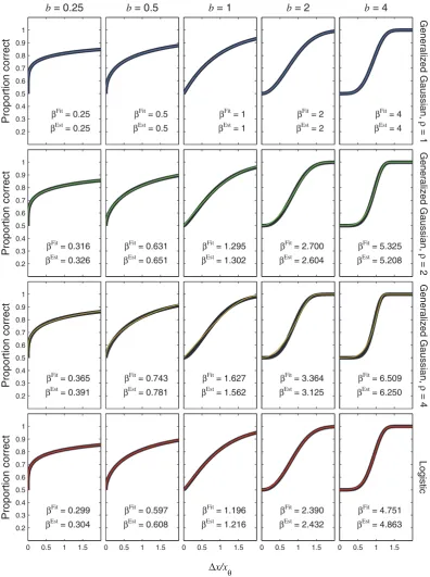
only in a linear horizontal scaling. The latter is useful when dealing with general cases where the threshold is not specified; the psychometric function is often expressed in this way [19,29,36]. The coloured curves in Figure 8 show the psychometric function of Equation (65). Different rows of panels show psychometric

functions for different noise CDFs,F, as indicated on the right

of the figure. Different columns of panels show psychometric

functions for different transducer exponents,b. The thick, black

curves show the best-fitting Weibull functions. These provide a good fit to the true psychometric functions, justifying the premise of Theorem 2, which is that the Weibull function provides a good fit.

Each panel of Figure 8 also compares b of the best-fitting

Weibull function (bFit) with the estimate, bEst, given by

bEst~bNoise|b. In every case, bEst is very close to the fitted value, the discrepancy being far smaller than the margin of error usually encountered in psychophysical measurements of psycho-metric function slope [22–27]. For each transducer (i.e. each

column of Figure 8), the difference inbEst between the different

noise CDFs (i.e. between the different rows of Figure 8) is caused

entirely by the different values ofbNoise. For example, the value of

bEstfor the Gaussian will always exceed that for the Laplace by a

factorbNoise_Gen:Gaussianð Þ2.bNoise_Gen:Gaussianð Þ1~1:302:

Power function and nonzero pedestal

We now consider the case of a power function and any pedestal value, a generalization of the previous case. First, starting with Equation (17), we trivially obtain

bTransducer_Powerfunc~b xpzDxh

b{1

Dxh

xpzDxh

b

{xpb

, ð66Þ

which reduces to Equation (63) whenxp~0. Whenxp=0, we can

start with Equation (35), from which it follows straightforwardly that

bTransducer_Powerfunc,xp=0~

bð1zWÞb{1W 1zW

ð Þb{1 : ð67Þ

Figure 9 plotsbTransducer_Powerfunc,xp=0as a function of the Weber fraction,

W(defined in Equation (34)), for several values of the transducer

exponent,b. These curves all converge to a value of 1 towards the

left. This is because, for a power function transducer with nonzero pedestal, the gradient of the transducer at the pedestal level is not 0 or‘, and so, as proved in Theorem 3, bTransducer_Powerfunc,xp=0?1 as W?0:

psychomet-0.2 0.3 0.4 0.5 0.6 0.7 0.8 0.9 1

Proportion correct

b = 0.25

βFit = 0.25

βEst _{= 0.25}

b = 0.5

βFit = 0.5

βEst _{= 0.5}

b = 1

βFit = 1

βEst _{= 1}

b = 2

βFit = 2

βEst _{= 2}

b = 4

βFit = 4

βEst _{= 4}

Generalized Gaussian,

ρ

= 1

0.2 0.3 0.4 0.5 0.6 0.7 0.8 0.9 1

Proportion correct β

Fit _{= 0.316}

βEst _{= 0.326}

βFit _{= 0.631}

βEst _{= 0.651}

βFit _{= 1.295}

βEst _{= 1.302}

βFit _{= 2.700}

βEst _{= 2.604}

βFit _{= 5.325}

βEst _{= 5.208}

Generalized Gaussian,

ρ

= 2

0.2 0.3 0.4 0.5 0.6 0.7 0.8 0.9 1

Proportion correct β

Fit _{= 0.365}

βEst _{= 0.391}

βFit _{= 0.743}

βEst _{= 0.781}

βFit _{= 1.627}

βEst _{= 1.562}

βFit _{= 3.364}

βEst _{= 3.125}

βFit _{= 6.509}

βEst _{= 6.250}

Generalized Gaussian,

ρ

= 4

0 0.5 1 1.5

0.2 0.3 0.4 0.5 0.6 0.7 0.8 0.9 1

Proportion correct β

Fit = 0.299

βEst _{= 0.304}

0 0.5 1 1.5

βFit = 0.597

βEst _{= 0.608}

0 0.5 1 1.5

βFit = 1.196

βEst _{= 1.216}

0 0.5 1 1.5

βFit = 2.390

βEst _{= 2.432}

0 0.5 1 1.5

βFit = 4.751

βEst _{= 4.863}

Logistic

Δx/x

θ

Figure 8. Psychometric functions resulting from power-function transducers and zero pedestal.The thin, coloured curves show the

psychometric function of Equation (65), plotted as a function ofDx=Dxh. Different rows of panels show psychometric functions with different noise CDFs,F, given by the Laplace distribution (top row of panels), the Gaussian (second row), the generalized Gaussian withr~4(third row) or logistic (bottom row). Different columns of panels show psychometric functions for different transducer exponents,b, as indicated at the top of the figure. The thick, black curves show the best-fitting (maximum-likelihood) Weibull functions. The curves in the middle column (b~1, top to bottom) are identical to Figures 7A to 7D, respectively. This is becauseb~1gives a linear transducer, and so the psychometric functions forb~1will have the same shape and same fittedbas the CDF (see Equation (10)). Each panel displays thebvalue of the best-fitting Weibull function (bFit) and the estimate,bEst_~bNoise_{|b, whereb}Noise_{is given by Equation (52), (53), (54) or (60), as appropriate.}