City, University of London Institutional Repository
Citation
:
Majewski, A. A., Bormetti, G. & Corsi, F. (2015). Smile from the past: A general option pricing framework with multiple volatility and leverage components. Journal of Econometrics, 187(2), pp. 521-532. doi: 10.1016/j.jeconom.2015.02.036This is the accepted version of the paper.
This version of the publication may differ from the final published
version.
Permanent repository link: http://openaccess.city.ac.uk/19452/
Link to published version
:
http://dx.doi.org/10.1016/j.jeconom.2015.02.036Copyright and reuse:
City Research Online aims to make research
outputs of City, University of London available to a wider audience.
Copyright and Moral Rights remain with the author(s) and/or copyright
holders. URLs from City Research Online may be freely distributed and
linked to.
Smile from the Past: A general option pricing framework
with multiple volatility and leverage components
Adam A. Majewskia,∗, Giacomo Bormettia,b, and Fulvio Corsic,d March 2014
a Scuola Normale Superiore, Piazza dei Cavalieri 7, Pisa, 56126, Italy
b QUANTLab1, via Pietrasantina 123, Pisa, 56122, Italy
c Ca’ Foscari University of Venice, Fondamenta San Giobbe 873, Venezia, 30121, Italy
dCity University London, Northampton Square, London EC1V 0HB, United Kingdom
Abstract
In the current literature, the analytical tractability of discrete time option pricing models is guaranteed only for rather specific types of models and pricing kernels. We propose a very general and fully analytical option pricing framework, encompassing a wide class of discrete time models featuring multiple-component structure in both volatility and leverage, and a flexible pricing kernel with multiple risk premia. Although the proposed framework is general enough to include either GARCH-type volatility, Realized Volatility or a combination of the two, in this paper we focus on realized volatility option pricing models by extending the Heterogeneous Autoregressive Gamma (HARG) model of Corsi et al. (2012) to incorporate heterogeneous leverage structures with multiple components, while preserving closed-form solutions for option prices. Applying our analytically tractable asymmetric HARG model to a large sample of S&P 500 index options, we demonstrate its superior ability to price out-of-the-money options compared to existing benchmarks.
∗
1
Introduction
Due primarily to mathematical tractability and flexibility of incorporating various types of risk premia,
the literature on option pricing traditionally has been dominated by continuous-time processes.2 On
the other hand, models for asset dynamics under the physical measure Phave primarily been
devel-oped in discrete-time. The time-varying volatility models of the ARCH-GARCH families (Engle, 1982;
Bollerslev, 1996; Glosten et al., 1993; Nelson, 1991) have led the field in estimating and predicting the
volatility dynamics. More recently, thanks to the availability of intra-day data, the so called Realized
Volatility (RV) approach also became a prominent approach for measuring and forecasting volatility.
The key advantage of the RV is that it provides a precise nonparametric measure of daily volatility3
(i.e., making it observable) which leads to simplicity in model estimation and superior forecasting
performance.
Discrete time models present the important advantage of being easily filtered and estimated even in the
presence of complex dynamical features such as long memory, multiple components and asymmetric
effects, which turns out to be crucial in improving volatility forecast and option pricing performances.
A growing strand of literature advocates for the presence of a multi-factor volatility structure both
under the physical measure (Muller et al., 1997; Engle and Lee, 1999; Bollerslev and Wright, 2001;
Barndorff-Nielsen and Shephard, 2001; Calvet and Fisher, 2004) and the risk neutral one (Bates, 2000,
2012; Li and Zhang, 2010; Christoffersen et al., 2008; Adrian and Rosenberg, 2007). In the discrete
time option pricing literature, multiple components have been incorporated into both GARCH-type
(Christoffersen et al., 2008) and realized volatility models (Corsi et al., 2012), and both approaches
have shown that short-run and long-run components are necessary to capture the term structure of
the implied volatility surface. Also in the modelling of the so called leverage effect (the asymmetric
impact of positive and negative past returns on future volatility), recent papers advocate the need
for a multi-component leverage structure in volatility forecasting (Scharth and Medeiros, 2009; Corsi
2
Heston (1993), Duan (1995), Heston and Nandi (2000), Merton (1976), Bates (1996), Bates (2000), Pan (2002), Huang (2004), Bates (2006), Eraker (2004), Eraker et al. (2003) and Broadie et al. (2007)
3
This idea trace back to Merton (1980) and has been recently formalized and generalized in a series of papers that apply the quadratic variation theory to the class ofL2semi-martingales; See, e.g., Comte and Renault (1998), Andersen
and Ren`o, 2012). Finally, the need for a flexible pricing kernel incorporating variance-dependent risk
premia, in addition to the common equity risk premium, has been well-documented by Christoffersen
et al. (2013). However, in the current literature, the analytical tractability of discrete time option
pricing models is guaranteed only for rather specific types of models and pricing kernels.
The purpose of this paper is to propose a very general framework encompassing a wide class of discrete
time multi-factor asymmetric volatility models for which we show how to derive (using conditional
moment-generating functions) closed-form option valuation formulas under a very general and
flex-ible state-dependent pricing kernel. This general framework allows for a wide range of interesting
applications. For instance, it permits a straightforward generalization of both the multi-component
GARCH-type model of Christoffersen et al. (2008) as well as of the Heterogeneous Autoregressive
Gamma (HARG) model for realized volatility of Corsi et al. (2012). In this paper we focus our
at-tention on the applications of the general framework to the realized volatility class of model, while its
applications to the GARCH type of model will be the subject of a separate, companion paper.4
In more detail, this paper provides several theoretical results for both the general framework and for
the specific application to realized volatility models which can be summarized as follows. For the
general framework we show: (i) the recursive formula for the analytical Moment Generating Function
(MGF) under P, (ii) the general characterization of the analytical no-arbitrage conditions, (iii) the
formal change of measure obtained using a general and flexible exponentially affine Stochastic
Dis-count Factor (SDF), which features both equity risk premium and multi-factor variance risk premia,
(iv) the recursive formula for the analytical MGF underQ.
In addition, by applying the general framework to the specific class of model featuring HARG type
dynamics for realized volatility we are able to: (i) introduce various flexible types of leverage with
heterogeneous structures analogous to the one specified by the HARG model for volatility, by
preserv-ing the full analytical tractability of the model, (ii) have flexible skewness and kurtosis term structure
under bothPandQ, (iii) have an explicit one-to-one mapping between the parameters of the volatility
dynamics under P and Q, (iv) have closed-form option prices for model with heterogeneous realized
volatility and leverage dynamics. Finally, by applying our fully analytically tractable HARG model
with heterogeneous leverage on a large sample of S&P 500 index options, we show the superior ability
of the model in pricing out-of-the-money (OTM) options compared to existing benchmarks.
The rest of the paper is organized as follows. In Section 2 we propose the general framework for option
pricing with multi-factor volatility models. Section 3 defines a family of HARG models for realized
volatility with leverage (LHARG), presents two particular models belonging to the family, describes
the estimation of the models, and analyzes their statistical properties. Section 4 reports the option
pricing performance of LHARG models, comparing them to benchmark models. Finally, in Section 5
we summarize the results.
2
The multi-factor volatility models
2.1 General framework
The main purpose of introducing a multi-factor structure in volatility modeling is to account for
de-pendencies among volatilities at different time-scales. Currently, there are two alternative approaches
in the literature. The first is to decompose the daily volatility into several factors and model the
dynamics of each factor independently, as done by Christoffersen et al. (2008) or Fouque and Lorig
(2011) in terms of short-run and long-run volatility components. The other approach is to define
factors as an average of past volatilities over different time horizons, for instance the daily, weekly and
monthly components in Corsi (2009). In this section we propose a general framework which includes
both approaches.
We consider a risky asset with priceSt and geometric return
yt+1= log
St+1 St
.
To model the dynamics of log-returns we define thek-dimensional vector of factors f1
t,. . ., ftk which
and the daily log-returns on dayt+ 1 are modeled by equation
yt+1 =r+λL(ft+1) +
p
L(ft+1) t+1, (2.1)
wherer is the risk-free rate, λis the market price of risk, and t are i.i.d. N (0,1). We modelft+1 as
ft+1|Ft,Lt∼ D(Θ0,Θ(Ft,Lt)), (2.2)
where D denotes a generic distribution depending on the vector of parameters Θ which is a
k-dimensional function of the matrices Ft = (ft, . . . ,ft−p+1) ∈ Rk×p and Lt = (`t, . . . ,`t−q+1) ∈ Rk×q
forp >0 andq >0, respectively. We consider the case of a linear dependence of Θ onF andL
Θ(Ft,Lt) =d+ p
X
i=1
Mift+1−i+ q
X
j=1
Nj`t+1−j, (2.3)
whereMi,Nj ∈Rk×k fori= 1, . . . , pand j= 1, . . . , q,d∈Rk, and vectors`t−j are of the form
`t+1−j =
t+1−j−γ1
p
L(ft+1−j)
2
.. .
t+1−j−γk
p
L(ft+1−j)
2
. (2.4)
The vector Θ0 collects all the parameters of the distribution D which do not depend on the past
history of the factors and of the leverage. For the distributionDconsidered in this paper (Dirac delta
and non-central Gamma distribution) the sufficient condition for the non-negativity of process reads:
d≥0 Mi≥0 for all i∈ {1, . . . , p} Nj ≥0 for all j∈ {1, . . . , q}, (2.5)
where≥has to be meant as componentwise inequality.
Assumption 1. The following relation holds true
Ehezys+1+b·fs+1+c·`s+1|F
s
i
= eA(z,b,c)+Pip=1Bi(z,b,c)·fs+1−i+Pqj=1Cj(z,b,c)·`s+1−j (2.6)
for some functionsA:R×Rk×Rk→R, B
i :R×Rk×Rk→Rk, andCj :R×Rk×Rk→Rk, where
b,c∈Rk and ·stands for the scalar product in Rk.
Our framework is suited to include both GARCH-like models and realized volatility models. As far as
the former class is concerned, we encompass the family of multiple component GARCH models with
parabolic leverage pioneered in Heston and Nandi (2000) and later extended to the two Component
GARCH (CGARCH) by Christoffersen et al. (2008). For instance, the latter model corresponds to
the following dynamics
yt+1 =r+λht+1+
p
ht+1t+1, ht+1 =qt+1+β1(ht−qt) +α1
2t −1−2γ1t
p
ht
,
qt+1 =ω+β2qt+α2
2t−1−2γ2t
p
ht
.
(2.7)
Settingk= 2, we define f1
t+1 =ht+1−qt+1 and ft2+1=qt+1 and rewrite the model as
f1 t+1 f2 t+1 =
−α1 ω−α2
+
β1−α1γ12 −α1γ12
−α2γ2
2 β2−α2γ22
f1 t f2 t +
α1 0
0 α2
t−γ1
p
L(ft)
2
t−γ2
p
L(ft)
2
, (2.8)
whereL(ft) = ft1+ ft2=ht. If we now specify forDin eq. (2.2) the form of a Dirac delta distribution,
define d = (−α1, ω−α2)t, and identify the matrices M1 and N1 in a natural way from the right term side of eq. (2.8), the model by Christoffersen et al. fits the general formula (2.2). It is worth
mentioning that for the CGARCH model it is not possible to ensure the non-negative definiteness
of both ht and qt for all t (condition (2.5) is not satisfied). Nonetheless, for realistic values of the
parameters the probability of obtaining negative volatility factors is extremely low, and this drawback
is largely compensated for by the effectiveness of the model in capturing real time series empirical
The second example that we discuss is the class of realized volatility models known as Autoregressive
Gamma Processes (ARG) introduced in Gourieroux and Jasiak (2006), to whom the Heterogeneous
Autoregressive Gamma (HARG) model presented in Corsi et al. (2012) belongs. The process RVt is
an ARG(p) if and only if its conditional distribution given (RVt−1, . . . ,RVt−p) is a noncentred gamma
distribution ¯γ(δ,Pp
i=1βiRVt−i, θ), where δ is the shape, Ppi=1βiRVt−i the non-centrality, andθ the
scale. Then, the model described by eq.s (2.2)-(2.3) reduces to an ARG(p) if we fix k= 1, ft= RVt,
D(Θ0,Θ(Ft−1)) = ¯γ(δ,Θ(Ft−1), θ) with
Θ0 = (δ, θ)t , and Θ(Ft−1) =
p
X
i=1
βift−i.
2.2 Physical and risk-neutral worlds
The general framework defined by eq.s (2.1)-(2.4) combined with the assumption (2.6) allows us to
completely characterize the MGF of the log-returns under the physical measure. If relation (2.6) is
satisfied, then the moment generating function of ln(ST/St) is given by recursive relation in terms of
functionsA,Bi,Cj: we present the formulae in Appendix B.
By specifying the Stochastic Discount Factor (SDF) within the family of the exponential-affine factors,
we are able to compute analogous recursions under Q. The need for variance-dependent risk premia
in SDF, in addition to the common equity risk premium, has been shown by Christoffersen et al.
(2013), Gagliardini et al. (2011) and Corsi et al. (2012) to be crucial in reconciling the time series
properties of stock returns with the cross-section of option prices. Our framework permits the adoption
of a very general and flexible pricing kernel incorporating, in addition to the common equity risk
premium, multiple factor-dependent risk premia. The most general SDF that we might consider in
our framework corresponds to the following
Ms,s+1 =
e−ν1·fs+1−ν2ys+1
EP[e−ν1·fs+1−ν2ys+1|Fs], (2.9)
realized variance. Thus we restrict to two risk premia, ν1 and ν2, leaving open the possibility for
future research to include further risk premia related to other volatility components due to jumps and
overnight returns.
Moment generating function under risk-neutral measure for models where the joint dynamics of
log-returns and volatiltiy is affine combined with exponential-affine SDF, can be derived in semi-closed
form, as has been shown in Gourieroux and Monfort (2007). In Appendix B we show that MGF of
ln(ST/St) under risk-neutral measure Qis given by recursive relation in terms of functionsA,Bi,Cj.
The resulting risk-neutral dynamics depend on the values of the equity and variance risk premia,ν1
and ν2 respectively, which have to satisfy the no arbitrage constraints. For all the models within the
general framework, the no-arbitrage conditions can be written in terms of functionsA,Bi,Cj given in
Propositon 2 which summarizes all the results of this section.
Proposition 2. If Assumption 1 is satisfied then the moment generating function of ln(ST/St) under
measures P and Q is given by recursive relation in terms of functions A, Bi, Cj. Moreover the
SDF (2.9) is compatible with the no arbitrage restriction if the following conditions are satisfied:
A(1−ν2,−ν1,0) =r+A(−ν2,−ν1,0)
Bi(1−ν2,−ν1,0) =Bi(−ν2,−ν1,0) for i= 1, . . . , p
Cj(1−ν2,−ν1,0) =Cj(−ν2,−ν1,0) for j= 1, . . . , q.
(2.10)
Proof: See Appendix A and B .
3
LHARG-RV
3.1 The model
HAR-RV processes were introduced to financial literature by Corsi (2009), and are characterized by
the different impact that past realized variances aggregated on a daily, weekly and monthly basis have
on today’s realized variance. Lagged terms are collected in three different non-overlapping factors: RVt
an extension of the HAR-RV which includes a daily binary Leverage component (HARGL). However,
in Corsi and Ren`o (2012) the authors stress the importance of a heterogeneous structure for leverage.
Thus we develop an Autoregressive Gamma model with Heterogeneous parabolic Leverage, and we
name it the LHARG-RV model.
LHARG-RV belongs to the family of models described by (2.1)-(2.4) setting k = 1 and ft = RVt.
Thus, log-returns evolve according to the equation
yt+1 =r+λRVt+1+
p
RVt+1t+1, (3.1)
while the realized variance at time t+ 1 conditioned on information at day t is sampled from a
noncentred gamma distribution
RVt+1|Ft∼¯γ(δ,Θ(RVt,Lt), θ) (3.2)
with
Θ(RVt,Lt) =d+βdRV
(d)
t +βwRV
(w)
t +βmRV
(m)
t +αd`
(d)
t +αw`
(w)
t +αm`
(m)
t . (3.3)
In the previous equationd∈Ris a constant and the quantities
RVt(d) = RVt, `t(d)= t−γ√RVt
2
,
RV(tw)= 1 4
P4
i=1RVt−i, `(tw)= 14
P4
i=1 t−i−γ√RVt−i
2
,
RV(tm)= 171 P21
i=5RVt−i, ` (m)
t = 171
P21
i=5 t−i−γ
√
RVt−i
2
,
correspond to the heterogeneous components associated with the short-term (daily), medium-term
(weekly), and long-term (monthly) volatility and leverage factors, on the left and right columns
re-spectively. The structure of leverage is analogous to the one in Heston and Nandi (2000), and it is
based on asymmetric influence of shock: large positive idiosyncratic componentthas a smaller impact
correlated:
Covt−1(yt, RVt+1) =−2θαdγE[RVt|Ft−1]
=−2θ2αdγ(δ+ Θ(RVt−1,Lt−1)).
(3.4)
In order to adjust eq. (3.3) to our framework we rewrite Θ(RVt,Lt) as
d+ 22
X
i=1
βiRVt+1−i+
22
X
j=1 αj
t+1−j−γ
p
RVt+1−j
2
, (3.5)
with
βi =
βd for i= 1
βw/4 for 2≤i≤5
βm/17 for 6≤i≤22
αj =
αd forj= 1
αw/4 for 2≤j≤5
αm/17 for 6≤j≤22
. (3.6)
We show in Appendix B that LHARG models satisfy Assumption 1, and we explicitly derive the A,
Bi, andCj functions. Then, the general results presented in Section 2.2 read
Proposition 3. Under P, the MGF for LHARG model has the following form
ϕP(t, T, z) =EP[ezyt,T|F
t] = exp
at+ p
X
i=1
bt,iRVt+1−i+ q
X
j=1
ct,j`t+1−j
(3.7)
where
as= as+1+zr− 1
2ln(1−2cs+1,1)−δW(xs+1, θ) +dV(xs+1, θ)
bs,i=
bs+1,i+1+V(xs+1, θ)βi for 1≤i≤p−1
V(xs+1, θ)βi for i=p
cs,j=
cs+1,j+1+V(xs+1, θ)αj for 1≤j≤q−1
V(xs+1, θ)αj for j=q
(3.8)
with
xs+1=zλ+ bs+1,1+ 1
2z2+γ2cs+1,1−2cs+1,1γz 1−2cs+1,1
The functionsV, W are defined as follows
V(x, θ) = θx
1−θx and W(x, θ) = ln (1−xθ) , (3.9)
and the terminal conditions readaT = bT ,i = cT ,j = 0 for i= 1, . . . , p and j= 1, . . . , q.
Proof: See Appendix C.
The proof of the previous proposition provides us with the explicit form of the functions A, Bi, and
Cj for the general class of LHARG models. Following the reasoning in Appendix F in Gourieroux and
Jasiak (2006) one can derive the stationarity condition forRVt process:
θ βd+βw+βm+γ2(αd+αw+αm)
<1. (3.10)
Employing the SDF suggested in (2.9), which for LHARG takes the form
Ms,s+1=
e−ν1RVs+1−ν2ys+1
EP[e−ν1RVs+1−ν2ys+1|F
s]
, (3.11)
and plugging theV and W functions in eq. (B.2) we readily obtain the risk-neutral MGF.
Corollary 4. Under the risk-neutral measure Qthe MGF for LHARG has the form
ϕQν1ν2(t, T, z) = exp
a∗t +
p
X
i=1
b∗t,iRVt+1−i+ q
X
j=1
c∗t,j`t+1−j
where
a∗s =a∗s+1+zr− 1
2ln(1−2c
∗
s+1,1)−δW(xs∗+1, θ) +δW(ys∗+1, θ) +dV(x∗s+1, θ)−dV(y∗s+1, θ)
b∗s,i=
b∗s+1,i+1+ V(xs∗+1, θ)− V(y∗s+1, θ)
βi for 1≤i≤p−1
V(x∗
s+1, θ)− V(y∗s+1, θ)
βi for i=p
c∗s,i=
c∗s+1,i+1+ V(xs∗+1, θ)− V(y∗s+1, θ)
αi for 1≤i≤q−1
V(x∗
s+1, θ)− V(y∗s+1, θ)
αi for i=q ,
(3.12)
with
x∗s+1 = (z−ν2)λ+ b∗s+1,1−ν1+ 1
2(z−ν2)
2+γ2c∗
s+1,1−2c∗s+1,1γ(z−ν2) 1−2c∗
s+1,1
,
y∗s+1 =−ν2λ−ν1+ 1 2ν
2 2,
and terminal conditions a∗T = b∗T ,i= c∗T,j = 0 for i= 1, . . . , pand j= 1, . . . , q.
Proof: See Appendix C.
The derivation of the no-arbitrage condition for LHARG readily follows from Proposition 2.
Corollary 5. The LHARG model defined by eq.s (3.1) and (3.3) with SDF specified as in (3.11)
satisfies the no-arbitrage condition if, and only if
ν2=λ+1
2. (3.13)
Proof: See Appendix C.
To derive the price of vanilla options, for example, it is sufficient to know the MGF under the
risk-neutral measureQwhich has been given in Corollary 4. However, for exotic instruments it is essential
to know the log-return dynamics under Q. The comparison of the physical and risk-neutral MGFs
into the dynamics underP.
Proposition 6. Under the risk-neutral measureQthe realized variance still follows a LHARG process
with parameters
βd∗ = 1
1−θy∗βd, βw∗ = 1−1θy∗βw, βm∗ = 1−1θy∗βm,
α∗d= 1−1θy∗αd, α∗w= 1−1θy∗αw, α∗m = 1−1θy∗αm,
θ∗ = 1
1−θy∗θ , δ∗ =δ , γ∗ =γ+λ+12,
d∗= 1−1θy∗d ,
(3.14)
where y∗=−λ2/2−ν1+1 8.
Proof: See Appendix D.
From the previous results we can write the simplified risk-neutral MGF which allows us to reduce the
computational burden when computing the backward recurrences.
Corollary 7. Under Q, the MGF for the LHARG model has the same form as in (3.7)-(3.8) with
equity risk premiumλ∗ =−0.5 and d∗, δ∗,θ∗, γ∗, α∗l,βl∗ for l=d, w, mas in (3.14).
3.2 Particular cases
We now discuss two special cases of the model presented in the previous section. The first instance is
the HARG model with Parabolic Leverage (P-LHARG) that we obtain setting d= 0 in (3.3), while
the second model is a LHARG with zero-mean leverage (ZM-LHARG). The shape of the leverage in
the latter has been inspired by the model of Christoffersen et al. (2008) but in the present context it
is enriched by a heterogeneous structure
¯
`(td)=2t −1−2tγ
p
RVt,
¯ `(tw)= 1
4 4
X
i=1
2t−i−1−2t−iγ
p
RVt−i
,
¯
`(tm)= 1 17
21
X
i=5
2t−i−1−2t−iγ
p
RVt−i
The linear Θ(RVt,Lt) in this case reads
βdRV(td)+βwRVt(w)+βmRV(tm)+αd`¯(td)+αw`¯t(w)+αm`¯(tm), (3.15)
which can be reduced to the form (3.3) setting d = −(αd+αw +αm), βl = βl −αlγ2 for l =
d, w, m. As will be more clear in the following section, the introduction of the less constrained leverage
allows the process to explain a larger fraction of the skewness and kurtosis observed in real data.
However, similarly to what has been discussed in Section 2 about Christoffersen et al. (2008), it is
no more guaranteed that the non centrality parameter of the gamma distribution is positive definite.
Nonetheless, in the next section we will provide numerical evidence of the effectiveness of our analytical
results in describing a regularized version of this model.
3.3 Estimation and statistical properties
The estimation of the parameters characterizing the LHARG-RV family is greatly simplified by the use
of Realized Volatility, which avoids any filtering procedure related to latent volatility processes. We
compute the RV from tick-by-tick data for the S&P 500 Futures, from January 1, 1990 to December
31, 2007. As pointed out in Corsi et al. (2012), the choice of an adequate RV estimator is mandatory
to reconcile the properties of LHARG-RV models with the realized volatility dynamics. Although
we aknowledge the importance of the jump contribution in log-returns and realized volatility5, these
components are not included in the class of models considered in this paper. In order to exclude the
effect of jump on log-return and volatility process, from the empirical analysis, we employ the same
methodology adopted by Corsi et al. (2012): i) we estimate the total variation of the log-prices using
the Two-Scale estimator proposed by Zhang et al. (2005); ii) purify it from the jump component in
prices by means of the Threshold Bipower variation method introduced in Corsi et al. (2010); iii)
re-move the most extreme observations (jumps) in the volatility series. Finally, to overcome the problem
of neglecting the contribution to the volatility due to the overnight effect we rescale our RV estimator
to match the unconditional mean of the squared close-to-close daily returns. Further details about
the construction of the RV measure are given in Corsi et al. (2012).
5
The use of an RV proxy for the unobservable volatility allows us simply to employ a Maximum
Likelihood Estimator (MLE) on historical data. Arguing as in Gourieroux and Jasiak (2006), the
conditional transition density for the LHARG-RV family is available in closed-form, and so the
log-likelihood reads
lTt(δ, θ, d, βd, βw, βm, αd, αw, αm, γ) =
−
T
X
t=1
RVt
θ + Θ (RVt−1,Lt−1)
+
T
X
t=1 log
∞
X
k=1
RVδt+k−1 θδ+kΓ(δ+k)
Θ (RVt−1,Lt−1)k
k!
!
where Θ (RVt−1,Lt−1) is given in eq. (3.3). To implement the MLE, we truncate the infinite sum on
the right hand side to the 90th order as done in Corsi et al. (2012). Finally, the estimation of the
market price of riskλ in the log-return eq. (3.2) is performed regressing the centred and normalized
log-returns on the realized volatility, in a similar way to eq. (18) in Corsi et al. (2012). As a proxy for
the risk-free rate r we employ the FED Fund rate.
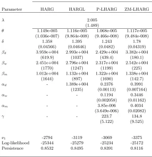
In Table 1 we report the parameter values estimated via maximum likelihood for four different models,
HARG, HARGL, P-LHARG, and ZM-LHARG6. We also show the parameter standard deviations (in
parenthesis), and the value of the log-likelihood. All parameters are statistically significant except the
monthly leverage component of P-LHARG. As already documented in Corsi (2009) and Corsi et al.
(2012) the RV coefficients show a decreasing impact of the past lags on the present value of the RV. As
far as the leverage components are concerned there is no evidence of a clear relation among different
lags. Finally, it is worth noting that the inclusion of leverage with heterogeneous structure improves
the likelihood of competitor HARG and HARGL models.
While we can ensure that P-LHARG model satisfies condition (2.5), for the ZM-LHARG model the
relation (3.15) cannot be prevented from obtaining negative values. Since the ZM-LHARG is worth
considering, we provide some numerical evidence supporting the analytical MGF as a reliable
approxi-mation of the MGF computed by simulation. We compare an extensive Monte Carlo (MC) simulation
of the ZM-LHARG dynamics where the non centrality parameter is artificially bounded from below (by
zero) with the analytical MGF computed according to Proposition 3. As the probability of obtaining a
6In Corsi et al. (2012) log-returns were expressed on a daily and percentage basis, whilst the realized volatility was
Model
Parameter HARG HARGL P-LHARG ZM-LHARG
λ 2.005
(1.489)
θ 1.149e-005 1.116e-005 1.068e-005 1.117e-005 (1.036e-007) (9.864e-008) (9.466e-008) (9.484e-008)
δ 1.358 1.395 1.243 1.78
(0.04566) (0.04646) (0.0482) (0.04319)
βd 3.959e+004 2.993e+004 2.429e+004 3.382e+004
(619.9) (1037) (439.4) (180.1)
βw 2.451e+004 2.796e+004 2.317e+004 2.542e+004
(1770) (1247) (1199) (225)
βm 1.012e+004 1.132e+004 1.322e+004 1.338e+004
(1644) (897) (1690) (142.7)
αd - 1.389e+004 0.2376 0.3991
(1235) (0.00113) (0.007164)
αw - - 0.1194 0.3446
(0.002058) (0.01162)
αm - - 3.85e-006 0.4034
(3.649e-006) (0.02082)
γ - - 223.7 134.8
(5.122) (9.525)
ν1 -2794 -3119 -3069 -3375
[image:17.612.144.456.120.442.2]Log-likelihood -25344 -25279 -25234 -25172 Persistence 0.8532 0.8495 0.8391 0.8116
Table 1: Maximum likelihood estimates, robust standard errors, and models’ performance. The historical data for the HARG, HARGL, P-LHARG and ZM-LHARG models are given by the daily RV measure computed on tick-by-tick data for the S&P500 Futures (see Section 3.3). For all three models, the estimation period ranges from 1990-2005. The parameter ν1 for each model has been fitted on option prices.
negative value for the non centrality of the gamma distribution is small (given the parameter values in
Table 1), we can assess that the analytical MGF is a good approximation of the unknown MGF of the
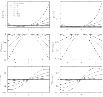
regularized ZM-LHARG. We fix the number of MC to 0.5×10⁶ and consider six relevant maturities,
one day (T = 1), one week (T = 5), one month (T = 22), one quarter (T = 63), six months (T = 126),
and one year (T = 256). In the left column from top to bottom of Figure 1 we plot the MGF, the real
and imaginary parts of the characteristic function under the physical measure, respectively, while in
−5 0 5 1 2 3 E P[e z yT ] Monte Carlo
T= 1
T= 5
T= 22
T= 63
T= 126 T= 252
−5 0 5
0.4 0.6 0.8 1 E P[cos ( z yT )]
−5 0 5
z −0.4
−0.2 0 0.2
E
P[sin(
z
yT
)]
−5 0 5
2.5 5 E Q[e z yT ]
−5 0 5
0.25 0.5 0.75 1 E Q[cos ( z yT )]
−5 0 5
z −0.4
−0.2 0 0.2
E
Q[sin(
z
yT
[image:18.612.99.507.172.556.2])]
0 100 200 T
0 0.5 1
Kurtosis
HARG HARGL P-LHARG ZM-LHARG
0 100 200
−0.5
−0.25
0
Sk
ewness
0 100 200
T 0
0.5 1
0 100 200
−0.5
−0.25
[image:19.612.97.508.105.366.2]0
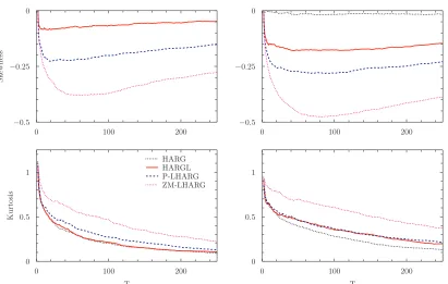
Figure 2: Left column, from top to bottom: skewness and excess kurtosis of the HARG, HARGL, P-LHARG, and ZM-LHARG processes under the physical measureP. Right column: same as the left column, but under the risk-neutral measure.
to the analytical MGFs while the MC expectations are represented by points whose size is larger than
the associated error bars. The quality of the agreement is extremely high. Moreover, the MC estimate
of the probability associated with the event Θ(RVt−1,Lt−1) < 0 is 2×10⁻⁵ under P, and 3×10⁻⁶ underQ, confirming once more the reliability of the approximation.
Crucial ingredients for reproducing the shape of the implied volatility surface are the term structure of
skewness and kurtosis generated by a given option pricing model. Therefore, in Figure 2 we compare
the skewness and excess kurtosis associated to the four models HARG, HARGL, P-LHARG, and
ZM-LHARG. We do not show the skewness for the HARG case under P, since this model is not
designed to explain the negative skewness. When moving to Q, the genuine effect of the calibration
of ν1 is to induce a small negative skewness. It is worth noticing that for the LHARG-RV models
adding the heterogeneous components not only improves the skewness upon the HARGL model, but
also considerably increases the excess kurtosis. As far as under the Q measure is concerned, the
ZM-LHARG always outperforms all the competitor models.
4
Valuation performance
4.1 Option pricing methodology
We apply the same option pricing procedure for both LHARG models, based on change of measure
described by (3.11), and MGF formula given by (3.7)-(3.8). To derive risk-neutral dynamics we need
to fix parameters of SDF, ν1 and ν2. While the latter is determined by the no-arbitrage condition
(Proposition 5), the former has to be calibrated on option prices. Following the same reasoning as Corsi
et al. (2012), we perform the unconditional calibration of ν1 such that the model generated and the
average market IV for a one-year time to maturity at-the-money option coincide.
We employ the option pricing numerical method termed COS, introduced by Fang and Oosterlee
(2008), and which has been proven to be efficient. The method is based on Fourier-cosine expansions
and is available as long as the characteristic function of log-returns is known. The numerical algorithm
exploits the close relation of the characteristic function with the series coefficients of Fourier-cosine
expansion of the density function.
To sum up, we proceed pricing options following four steps: (i) estimation under the physical measure
P, (ii) unconditional calibration of the parameter ν1 (iii) mapping of the parameters of the model estimated under Pinto the parameters underQ, and (iv) approximation of option prices by the COS
method using the MGF formula in (3.7)-(3.8) with parameters under measureQ.
4.2 Results
In this section we present empirical results for option pricing with LHARG models. For the sake of
completeness we also compare LHARG models with the HARG model with no leverage and with the
HARGL presented in Corsi et al. (2012). Since the functional form of the leverage of the latter model
pricing are not available. Thus, we resort to numerical methodologies such as extensive Monte Carlo
scenario generation.
We perform our analysis on European options, written on the S&P 500 index. The time series of
option prices range from January 1, 1996 to December 31, 2004 and the data are downloaded from
OptionMetrics. As is customary in the literature (see Barone-Adesi et al. (2008)), we filter out options
with time to maturity less than 10 days or more than 365 days, implied volatility larger than 70%, and
prices less than 5 cents. Following Corsi et al. (2012), we consider only out-of-the-money (OTM) put
and call options for each Wednesday. Moreover we discard deep out-of-the-money options (moneyness
larger than 1.2 for call options and less than 0.8 for put options). The procedure yields a total of
41536 observations.
As a measure of the option pricing performance we use the percentage Implied Volatility Root Mean
Square Error (RM SEIV) put forward by Renault (1997) and computed as
RM SEIV =
v u u t
1 N
N
X
i=1
IVmkt
i −IVimod
2
×100,
whereN is the number of options,IVmktand IVmodrepresent the market and model implied
volatil-ities, respectively. An alternative performance measure corresponds to the Price Root Mean Square
Error (RM SEP) defined in a similar way asRM SEIV but with implied volatilities replaced by relative
prices. We employ the RM SEIV measure since it tends to put more weight on OTM options, while
theRM SEP emphasizes the importance of ATM options.
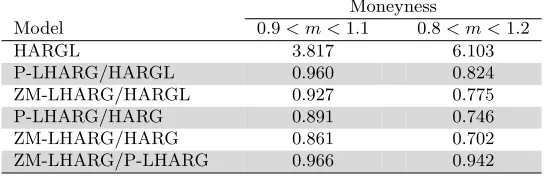
The result of our empirical analysis is that both LHARG models outperform competing RV-based
stochastic volatility models (HARG, HARGL). Table 2 shows that P-LHARG outperforms HARG
and HARGL by about 11% and 4%, respectively, in range of moneyness 0.9 < m < 1.1 and by
about 35% and 17%, respectively, in range of moneyness 0.8 < m < 1.2. ZM-LHARG outperforms
HARG and HARGL by about 14% and 7%, respectively, in range of moneyness 0.9 < m < 1.1 and
Implied Volatility RMSE
Moneyness
Model 0.9< m <1.1 0.8< m <1.2
HARGL 3.817 6.103
P-LHARG/HARGL 0.960 0.824
ZM-LHARG/HARGL 0.927 0.775
P-LHARG/HARG 0.891 0.746
ZM-LHARG/HARG 0.861 0.702
[image:22.612.163.435.136.224.2]ZM-LHARG/P-LHARG 0.966 0.942
Table 2: Global option pricing performance on S&P500 out-of-the-money options from January 1, 1996 to December 31, 2004, computed with the RV measure estimated from 1990 to 2007.
We use the maximum likelihood parameter estimates from Table 1. First row: percentage implied volatility root mean squared error (RM SEIV) of the HARGL model (benchmark) for different
mon-eyness range.Second and subsequent rows: relative RM SEIV of the selected models.
P-LHARG by about 3% and 6%, in range of moneyness 0.9< m <1.1 and 0.8< m <1.2, respectively.
The detailed analysis in Table 3 confirms that the main advantage of LHARG models is the ability
to capture the volatility smile. While the performance of all models in the at-the-money region is
similar, both LHARG models significantly outperform HARG and HARGL in the range of moneyness
1.1< m <1.2 and even more at the put side region 0.8< m <0.9. This improvement stems from the
higher flexibility of the model obtained with a multi-component leverage structure.
Panel B of Table 3 compares the performance of HARGL and P-LHARG. It shows the advantage
of heterogeneous leverage compared to one-day binary leverage. Improvement for short maturities
and moneyness 0.8 < m <0.9 reaches about 30%. For longer maturities and moneyness below 0.9,
P-LHARG still outperforms HARGL, obtaining 3%−8% smaller RM SEIV. In the other moneyness
regions the two models perform quite similarly.
The ratio between RM SEIV of HARGL and ZM-LHARG is displayed in Panel C of Table 3. The
advantage of zero-mean heterogeneous leverage over one-day binary leverage is even stronger than in
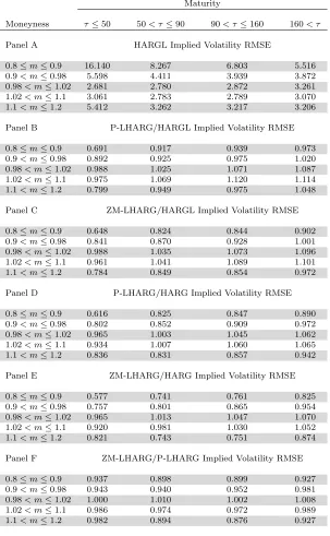
Maturity
Moneyness τ≤50 50< τ≤90 90< τ≤160 160< τ
Panel A HARGL Implied Volatility RMSE
0.8≤m≤0.9 16.140 8.267 6.803 5.516 0.9< m≤0.98 5.598 4.411 3.939 3.872 0.98< m≤1.02 2.681 2.780 2.872 3.261 1.02< m≤1.1 3.061 2.783 2.789 3.070 1.1< m≤1.2 5.412 3.262 3.217 3.206 Panel B P-LHARG/HARGL Implied Volatility RMSE
0.8≤m≤0.9 0.691 0.917 0.939 0.973 0.9< m≤0.98 0.892 0.925 0.975 1.020 0.98< m≤1.02 0.988 1.025 1.071 1.087 1.02< m≤1.1 0.975 1.069 1.120 1.114 1.1< m≤1.2 0.799 0.949 0.975 1.048 Panel C ZM-LHARG/HARGL Implied Volatility RMSE
0.8≤m≤0.9 0.648 0.824 0.844 0.902 0.9< m≤0.98 0.841 0.870 0.928 1.001 0.98< m≤1.02 0.988 1.035 1.073 1.096 1.02< m≤1.1 0.961 1.041 1.089 1.101 1.1< m≤1.2 0.784 0.849 0.854 0.972 Panel D P-LHARG/HARG Implied Volatility RMSE
0.8≤m≤0.9 0.616 0.825 0.847 0.890 0.9< m≤0.98 0.802 0.852 0.909 0.972 0.98< m≤1.02 0.965 1.003 1.045 1.062 1.02< m≤1.1 0.934 1.007 1.060 1.065 1.1< m≤1.2 0.836 0.831 0.857 0.942 Panel E ZM-LHARG/HARG Implied Volatility RMSE
0.8≤m≤0.9 0.577 0.741 0.761 0.825 0.9< m≤0.98 0.757 0.801 0.865 0.954 0.98< m≤1.02 0.965 1.013 1.047 1.070 1.02< m≤1.1 0.920 0.981 1.030 1.052 1.1< m≤1.2 0.821 0.743 0.751 0.874 Panel F ZM-LHARG/P-LHARG Implied Volatility RMSE
[image:23.612.149.452.118.609.2]0.8≤m≤0.9 0.937 0.898 0.899 0.927 0.9< m≤0.98 0.943 0.940 0.952 0.981 0.98< m≤1.02 1.000 1.010 1.002 1.008 1.02< m≤1.1 0.986 0.974 0.972 0.989 1.1< m≤1.2 0.982 0.894 0.876 0.927
Table 3: Option pricing performance on S&P500 out-of-the-money options from January 1, 1996 to December 31, 2004, computed with the RV measure estimated from 1990 to 2007.
We use the maximum likelihood parameter estimates from Table 1. Panel A: percentage implied volatility root mean squared error (RM SEIV) of the HARGL model sorted by moneyness and
0.9 we obtain about 35% improvement. ZM-LHARG also performs better for deep out-of-the-money
options on call side (1.1< m <1.2), where improvement varies from 3% to 22%.
Comparing model HARG without leverage with P-LHARG and ZM-LHARG in Panel D and Panel
E, respectively, the superiority of the latter two is even more apparent. While the performance
for the ATM options is comparable, the OTM options models with heterogeneous leverage generate
considerable improvement over models without leverage. In the extreme case of OTM short maturity
put options P-LHARG and ZM-LHARG produces errors which are smaller by 38% - 42%, respectively.
The last Panel (F) of Table 3 compares ZM-LHARG with P-LHARG. It shows that the ability of
ZM-LHARG model to reproduce higher levels of skewness and kurtosis, permits this more flexible
model to outperform the more constrained P-LHARG model. The outperformance is systematic, from
ATM options, whereRM SEIV is essentially the same, to deep out-of-the-money (m >1.1 orm <0.9)
whereRM SEIV is smaller by about 10%.
To summarize, the proposed LHARG models are better able to reproduce the IV level for OTM
options, improving upon the considered HARG and HARGL models. The heterogeneous structure of
the leverage thus appears to be a necessary ingredient for more accurate modeling of the IV smile.
5
Conclusions
In this paper we propose a very general framework which includes a wide class of discrete time
models featuring multiple components structure in both volatility and leverage and a flexible pricing
kernel with multiple risk premia. Within this framework we characterize the recursive formulae for
the analytical MGF under P and Q, the change of measure obtained using a flexible exponentially
affine SDF, and the analytical no-arbitrage conditions. Then, we focus on a specific new class of
realized volatility models, named LHARG, which extend the HARGL model of Corsi et al. (2012) to
incorporate analytically tractable heterogeneous leverage structures with multiple components. This
proposed general framework can be employed to include several additional features like jumps in
log-return and realized volatility, overnight effect, combination of GARCH and realized volatility models,
and switching in volatility regimes.
Acknowledgements
All authors warmly thank Nicola Fusari and Davide La Vecchia for helpful comments and fruitful
discussions and anonymous referees for helpful remarks. Additionally, we would like to thank Peter
Lieberman for the help in text editing.
References
Adrian, T., Rosenberg, J., 2007. Stock returns and volatility: Pricing the long-run and short-run components of market risk. Journal of Finance, forthcoming.
Andersen, T. G., Bollerslev, T., Diebold, F., 2007. Roughing it up: Including jump components in the measurement, modeling and forecasting of return volatility. Review of Economics and Statistics 89, 701–720.
Andersen, T. G., Bollerslev, T., Diebold, F., Labys, P., 2001. The distribution of realized exchange rate volatility. Journal of the American Statistical Association 96, 42–55.
Andersen, T. G., Bollerslev, T., Diebold, F., Labys, P., 2003. Modeling and forecasting realized volatility. Econometrica 71, 579–625.
Barndorff-Nielsen, O. E., Shephard, N., 2001. Non-Gaussian Ornstein-Uhlenbeck-based models and some of their uses in financial economics. Journal of the Royal Statistical Society Series B (63), 167–241.
Barndorff-Nielsen, O. E., Shephard, N., 2002a. Econometric analysis of realized volatility and its use in estimating stochastic volatility models. Journal of the Royal Statistical Society: Series B (Statistical Methodology) 64, 253–280.
Barndorff-Nielsen, O. E., Shephard, N., 2002b. Estimating quadratic variation using realized variance. Journal of Applied Econometrics 17, 457–477.
Barndorff-Nielsen, O. E., Shephard, N., 2005. How accurate is the asymptotic approximation to the distribution of realized volatility? In: Andrews, D. W. F., Stock, J. H. (Eds.), Identification and Inference for Econometric Models. A Festschrift in Honour of T.J. Rothenberg. Cambridge University Press, pp. 306–331.
Barndorff-Nielsen, O. E., Shephard, N., 2006. Econometrics of testing for jumps in financial economics using bipower variation. Journal of financial Econometrics 4 (1), 1–30.
Barone-Adesi, G., Engle, R., Mancini, L., 2008. A GARCH option pricing with filtered historical simulation. Review of Financial Studies 21, 1223–1258.
Bates, D., 1996. Jumps and stochastic volatility: Exchange rate processes implicit in Deutsche Mark options. Review of Financial Studies 9, 69–107.
Bates, D., 2000. Post-’87 crash fears in the S&P 500 futures option market. Journal of Econometrics 94 (1-2), 181–238.
Bates, D. S., 2012. US stock market crash risk, 1926–2010. Journal of Financial Economics 105 (2), 229–259.
Bollerslev, T., 1996. Generalize Autoregressive Conditional Heteroskedasticity. Journal of Econometrics 31, 307–327.
Bollerslev, T., Wright, J., 2001. Volatility forecasting, high-frequency data, and frequency domain inference. Review of Economics and Statistics 83, 596–602.
Broadie, M., Chernov, M., Johannes, M., 2007. Model specification and risk premia: Evidence from futures options. Journal of Finance 62, 1453–1490.
Calvet, L., Fisher, A., 2004. How to forecast long-run volatility: Regime switching and the estimation of multifractal processes. Journal of Financial Econometrics 2 (1), 49–83.
Christoffersen, P., Feunou, B., Jacobs, K., Meddahi, N., 2014. The economic value of realized volatility: Using high-frequency returns for option valuation. Journal of Financial and Quantitative Analysis 49 (03), 663–697.
Christoffersen, P., Heston, S., Jacobs, K., 2013. Capturing option anomalies with a variance-dependent pricing kernel. Review of Financial Studies, hht033.
Christoffersen, P., Jacobs, K., Ornthanalai, C., Wang, Y., 2008. Option valuation with long-run and short-run volatility components. Journal of Financial Economics 90 (3), 272–297.
Comte, F., Renault, E., 1998. Long memory in continuous time stochastic volatility models. Mathematical Finance 8, 291–323.
Corsi, F., 2009. A simple approximate long-memory model of realized-volatility. Journal of Financial Econometrics 7, 174–196.
Corsi, F., Fusari, N., La Vecchia, D., 2012. Realizing smiles: Options pricing with realized volatility. Journal of Financial Economics.
Corsi, F., Pirino, D., Ren`o, R., 2010. Threshold bipower variation and the impact of jumps on volatility forecasting. Journal of Econometrics 159 (2), 276 – 288.
Corsi, F., Ren`o, R., 2012. Discrete-time volatility forecasting with persistent leverage effect and the link with continuous-time volatility modeling. Journal of Business & Economic Statistics 30 (3), 368–380.
Duan, J. C., 1995. The GARCH option pricing model. Mathematical Finance 5, 13–32.
Engle, R., 1982. Autoregressive conditional heteroskedasticity with estimation of the variance of UK inflation. Econo-metrica 50, 987–1008.
Engle, R., Lee, G., 1999. A permanent and transitory component model of stock return volatility, in ed. R. Engle and H. White Cointegration, Causality, and Forecasting: A Festschrift in Honor of Clive W. J. Granger.
Eraker, B., 2004. Do stock prices and volatility jump? Reconciling evidence from spot and option prices. Journal of Finance 59, 1367–1403.
Eraker, B., Johannes, M., Polson, N., 2003. The impact of jumps in volatility and returns. Journal of Finance 58, 1269–1300.
Fang, F., Oosterlee, C. W., 2008. A novel pricing method for european options based on Fourier-Cosine series expansions. SIAM Journal on Scientific Computing 31, 826–848.
Fouque, J.-P., Lorig, M. J., 2011. A fast mean-reverting correction to Heston’s stochastic volatility model. SIAM Journal on Financial Mathematics 2 (1), 221–254.
Glosten, L. R., Jagannathan, R., Runkle, D., 1993. On the relation between the expected value and the volatility of the nominal excess return on stocks. Journal of Finance 48, 1779–1801.
Gourieroux, C., Jasiak, J., 2006. Autoregressive gamma process. Journal of Forecasting 25, 129–152.
Gourieroux, C., Monfort, A., 2007. Econometric specification of stochastic discount factor models. Journal of Economet-rics 136 (2), 509–530.
Heston, L. S., 1993. Options with stochastic volatiltiy with applications to bond and currency options. The Review of Fiancial Studies 6, 327–343.
Heston, S., Nandi, S., 2000. A closed-form GARCH option valuation model. Review Financial Studies 13 (3), 585–625.
Huang, X. Wu, L., 2004. Specification analysis of option pricing models based on time-changed L´evy processes. Journal of Finance 59, 1405–1439.
Li, G., Zhang, C., 2010. On the number of state variables in options pricing. Management Science 56 (11), 2058.
Merton, R. C., 1976. Option pricing when underlying stock returns are discontinuosus. Journal of Financial Economics 3, 125–144.
Merton, R. C., 1980. On estimating the expected return on the market: An exploratory investigation. Journal of Financial Economics 8, 323–61.
Muller, U., Dacorogna, M., Dav´e, R., Olsen, R., Pictet, O., von Weizsacker, J., 1997. Volatilities of different time resolutions - analyzing the dynamics of market components. Journal of Empirical Finance 4, 213–239.
Nelson, D. B., 1991. Conditional heteroskedasticity in asset returns: A new approach. Econometrica 59, 347–370.
Pan, J., 2002. The jump-risk premia implicit in options: Evidence from an integrateed time-series study. Journal of Financial Economics 63, 3–50.
Renault, E., 1997. Econometric models of option pricing errors. Econometric Society Monographs 28, 223–278.
Scharth, M., Medeiros, M. C., 2009. Asymmetric effects and long memory in the volatility of Dow Jones stocks. Interna-tional Journal of Forecasting 25 (2), 304–327.
Zhang, L., A¨ıt-Sahalia, Y., Mykland, P. A., 2005. A tale of two time scales: Determining integrated volatility with noisy high frequency data. Journal of the American Statistical Association 100, 1394–1411.
A
No arbitrage condition
The no-arbitrage conditions are
EP[Ms,s+1|Fs] = 1 fors∈Z+, (A.1)
The first condition is satisfied by definition of Ms,s+1. Before moving to the second condition, let us
rewrite the SDF as
Ms,s+1=
e−ν1·fs+1−ν2ys+1
EP[e−ν1·fs+1−ν2ys+1|F
s] = exp
− A(−ν2,−ν1,0)−
p
X
i=1
Bi(−ν2,−ν1,0)·fs+1−i
−
q
X
i=1
Ci(−ν2,−ν1,0)·`s+1−i−ν1·fs+1−ν2ys+1
, (A.3)
whereν1= (ν1, . . . , ν1)t∈Rk and functionsA,B
i andCj are defined in (2.6). Finally, the condition
(A.2) reads
EP[exp (−ν
1·fs+1+ (1−ν2)ys+1)|Fs]
= exp
r+A(−ν2,−ν1,0) +
p
X
i=1
Bi(−ν2,−ν1,0)·fs+1−i+
q
X
j=1
Cj(−ν2,−ν1,0)·`s+1−j
.
(A.4)
Using once again the relation (2.6) we obtain the no-arbitrage conditions.
B
Computation of MGF
Under the risk-neutral measure Q the MGF of the log-returns yt,T = log(ST/St) conditional on the
information available at timetis of the form
ϕQν1ν2(t, T, z) = ea∗t+
Pp
i=1b
∗
t,i·ft+1−i+Pqj=1c
∗
t,j·`t+1−j , (B.1)
where
a∗s= a∗s+1+A(z−ν2,b∗s+1,1−ν1,c∗s+1,1)− A(−ν2,−ν1,0)
b∗s,i=
b∗s+1,i+1+Bi(z−ν2,b∗s+1,1−ν1,cs∗+1,1)−Bi(−ν2,−ν1,0) if 1≤i≤p−1
Bi(z−ν2,b∗s+1,1−ν1,c∗s+1,1)−Bi(−ν2,−ν1,0) ifi=p
c∗s,j=
c∗s+1,j+1+Cj(z−ν2,b∗s+1,1−ν1,cs∗+1,1)−Cj(−ν2,−ν1,0) if 1≤j≤q−1
Cj(z−ν2,b∗s+1,1−ν1,c∗s+1,1)−Cj(−ν2,−ν1,0) ifj=q
(B.2)
and a∗
T = 0, b
∗
The above relation can be derived using the expression for the SDF given in (A.3), repeatedly and using the tower law of conditional expectation we obtain
ϕQν1ν2(t, T, z) =EQ[ezyt,T|F
t]
=EP[Mt,t+1. . . MT−1,Tezyt,T|Ft]
=EPhMt,t+1. . . MT−2,T−1ezyt,T−1EP[MT−1,TezyT|FT−1]|Ft
i
=EP
Mt,t+1. . . MT−2,T−1ezyt,T−1−A(−ν2,−ν1,0)−
Pp
i=1Bi(−ν2,−ν1,0)·fT−i ×e−Pqj=1Cj(−ν2,−ν1,0)·`T−iEPhe−ν1·fT+(z−ν2)yT|F
T−1
i |Ft
=EP
"
Mt,t+1. . . MT−2,T−1ezyt,T−1+A(z−ν2,−ν1,0)−A(−ν2,−ν1,0)
×ePpi=1[Bi(z−ν2,−ν1,0)−Bi(−ν2,−ν1,0)]·fT−i+Pqj=1[Cj(z−ν2,−ν1,0)−Cj(−ν2,−ν1,0)]·`T−j|Ft
#
=EPhMt,t+1. . . MT−2,T−1ezyt,T−1+a
∗
T−1+
Pp
i=1b
∗
T−1,i·fT−i+Pjq=1c∗T−1,j·`T−j|F
t
i
=EP
Mt,t+1. . . MT−3,T−2ezyt,T−2+a
∗
T−1
×EPhMT−2,T−1ezyT−1+
Pp i=1b
∗
T−1,i·fT−i+Pjq=1c∗T−1,j·`T−j |FT−2
i|Ft
=. . .
= ea∗t+
Pp i=1b
∗
t,i·ft+1−i+Pjq=1c∗t,j·`t+1−j.
Finally, the MGF under P readily follows by noticing that for ν1 =ν2 = 0 the SDF reduces to one, thereforeϕP(t, T, z) =ϕQ00(t, T, z).
C
MGF computation for LHARG and no-arbitrage conditions
Firstly, we derive the explicit form of the scalar functions A, Bi and Cj. In the case of LHARG we
have ft= RVt. Then,
EPhezys+bRVs+c`s|F
s−1
i
= ezrEPhe(zλ+b)RVsEPhez √
RVss+c(s−γ √
RVs)2|RV
s
i
|Fs−1
i
= ezrEP
e
zλ+b−z2
4c+γz
RVs
EPhec(s−(γ−2zc) √
RVs)2|RV
s
i
|Fs−1
= ezr−12ln(1−2c)EP
"
e
zλ+b+
1
2z2+γ2c−2cγz 1−2c
RVs |Fs−1
#
.
In the last equality we have used the fact that ifZ ∼ N(0,1) then
E
exp x(Z+y)2
= exp
−1
2ln(1−2x) + xy2 1−2x
. (C.2)
Using eq.s (8)-(9) from Gourieroux and Jasiak (2006) we obtain
EPhezys+bRVs+c`s|F
s−1
i
= exp
zr−
1
2ln(1−2c)−δW(x, θ) +V(x, θ)
d+
p
X
i=1
βiRVs−i+ q
X
j=1 αj`s−j
,
(C.3)
where
V(x, θ) = θx
1−θx, W(x, θ) = ln (1−xθ) , and
x(z, b, c) =zλ+b+ 1
2z2+γ2c−2cγz 1−2c .
From a direct inspection of the relation (2.6), we conclude that
A(z, b, c) =zr−1
2ln(1−2c)−δW(x, θ) +dV(x, θ),
Bi(z, b, c) =V(x, θ)βi,
Cj(z, b, c) =V(x, θ)αj.
(C.4)
Finally, plugging the above expressions forA,Bi and Cj in eq. (B.2) we readily obtain the recurrence
relations under the physical and risk-neutral measures. The no-arbitrage condition similarly follows from formulae (C.4) and relations (2.10) noticing that it is sufficient to impose
x(1−ν2,−ν1,0) =x(−ν2,−ν1,0).
D
Risk-neutral dynamics
To derive the mapping of the parameters under which the risk-neutral MGF is formally equivalent to the physical MGF, we need to compare eq. (3.12) to eq. (3.8). In particular we have to find a set of starred parameters for which the recursions under P correspond to the expressions under Q. More precisely, after defining
x∗∗s+1=zλ∗+ b∗s+1,1+ 1 2z
2+ (γ∗)2c∗
the following relations have to hold
δ W(x∗s+1, θ)− W(y∗, θ)
=δ∗W(x∗∗
s+1, θ∗), (D.1) βi V(x∗s+1, θ)− V(y∗, θ)
=β∗
iV(x∗∗s+1, θ∗), (D.2) αj V(x∗s+1, θ)− V(y
∗, θ)
=α∗
jV(x∗∗s+1, θ∗), (D.3) d V(x∗s+1, θ)− V(y∗, θ)
=d∗V(x∗∗s+1, θ∗), (D.4)
with y∗ =−λ2/2−ν
1+ 18. Eq. (D.1) can be rewritten as
δlog
1− θ 1−θy∗ x
∗
s+1−y∗
=δ∗log 1−θ∗x∗∗s+1
,
from which we obtain the sufficient conditions δ∗ = δ, θ∗ = θ/(1−θy∗), and x∗
s+1 −y∗ = x∗∗s+1. It is possible to verify by substitution that the latter relation is satisfied posing λ∗ = −1/2 and γ∗ =γ+λ+ 1/2. The relation (D.2) is equivalent to
βi
1−θy∗
θ 1−θy∗
x∗s+1−y∗
1−θ/(1−θy∗) x∗
s+1−y∗
=β
∗
i
θ∗x∗∗s+1 1−θ∗x∗∗
s+1 ,
which impliesβ∗