Multiple-plane particle image velocimetry using a light-field camera

City, University of London Institutional Repository

Citation

:

Skupsch, C. & Brücker, C. (2013). Multiple-plane particle image velocimetry

using a light-field camera. Optics Express, 21(2), pp. 1726-1740. doi:

10.1364/OE.21.001726

This is the accepted version of the paper.

This version of the publication may differ from the final published

version.

Permanent repository link:

http://openaccess.city.ac.uk/16750/

Link to published version

:

http://dx.doi.org/10.1364/OE.21.001726

Copyright and reuse:

City Research Online aims to make research

outputs of City, University of London available to a wider audience.

Copyright and Moral Rights remain with the author(s) and/or copyright

holders. URLs from City Research Online may be freely distributed and

linked to.

City Research Online:

http://openaccess.city.ac.uk/

[email protected]

Multiple-plane particle image velocimetry using

a light-field camera

Christoph Skupsch,1,* Christoph Brücker1

1 _{Technical University Bergakademie Freiberg, Department for Mechanics and Fluid Dynamics, Lampadiusstr. 4,}

09596 Freiberg/Saxony, Germany *_{[email protected]}

Abstract: Planar velocity fields in flows are determined on parallel measurement planes simultaneously by means of an in-house manufactured light-field camera. The planes are defined by illuminating light sheets with constant spacing. Particle positions are reconstructed from a single 2D recording taken by a CMOS-camera equipped with a high-quality doublet lens array. The fast refocusing algorithm bases on synthetic-aperture particle image velocimetry (SAPIV). Reconstruction quality is tested by ray-tracing of synthetically generated particle fields. Influence of image processing is documented. The introduced single-camera SAPIV is applied to a convective flow within a measurement volume of 30x30x50mm³.

2012 Optical Society of America

OCIS codes: (100.6890) Three-dimensional image processing; (110.0100) Imaging systems; (110.6880) Three-dimensional image acquisition; (280.7250) Velocimetry.

References and links

1. C. E. Willert and M. Gharib, “Digital particle image velocimetry,” Experiments in Fluids 10, 181–193 (1991). 2. K. D. Hinsch, “Three-dimensional particle velocimetry,” Meas. Sci. Technol 6, 742–753 (1995).

3. C. J. Kähler and J. Kompenhans, “Fundamentals of multiple plane stereo particle image velocimetry,” Experiments in Fluids 29, S070 (2000).

4. C. Brücker, “3-D PIV via spatial correlation in a color-coded light-sheet,” Exp Fluids 21, 312–314 (1996). 5. J. A. Mullin and W. J. A. Dahm, “Dual-plane stereo particle image velocimetry (DSPIV) for measuring velocity

gradient fields at intermediate and small scales of turbulent flows,” Exp Fluids 38, 185–196 (2005). 6. C. Brücker, “Digital-Particle-Image-Velocimetry (DPIV) in a scanning light-sheet: 3D starting flow around a

short cylinder,” Experiments in Fluids 19, 255–263 (1995).

7. V. Palero, J. Lobera, and M. P. Arroyo, “Digital image plane holography (DIPH) for two-phase flow diagnostics in multiple planes,” Exp Fluids 39, 397–406 (2005).

8. A. Liberzon, R. Gurka, and G. Hetsroni, “XPIV-Multi-plane stereoscopic particle image velocimetry,” Experiments in Fluids 36, 355–362 (2004).

9. G. E. Elsinga, F. Scarano, B. Wieneke, and B. W. Oudheusden, “Tomographic particle image velocimetry,” Exp Fluids 41, 933–947 (2006).

10. F. Pereira and M. Gharib, “Defocusing digital particle image velocimetry and the three-dimensional characterization of two-phase flows,” Measurement Science and Technology 13, 683–694 (2002). 11. C. Cierpka, R. Segura, R. Hain, and C. J. Kähler, “A simple single camera 3C3D velocity measurement

technique without errors due to depth of correlation and spatial averaging for microfluidics,” Meas. Sci. Technol. 21, 45401 (2010).

12. J. Belden, T. T. Truscott, M. C. Axiak, and A. H. Techet, “Three-dimensional synthetic aperture particle image velocimetry,” Meas. Sci. Technol 21, 125403 (2010).

13. B. Wilburn, Joshi N., Vaish V., Talvala E. V., Antunez E., Barth A., Adams A., Horowitz M., and Levoy M., “High performance imaging using large camera arrays,” ACM Transactions on Graphics 24 (2005). 14. M. Levoy, “Light fields and computational imaging,” Computer 39, 46–55 (2006).

16. T. Nonn, J. Kitzhofer, D. Hess, and C. Brücker, “Measurements in an IC-engine Flow using Light-field Volumetric Velocimetry,” in Proceedings of 16th Int Symp on Applications of Laser Techniques to Fluid Mechanics, Lisbon, Portugal, 9-12 July 2012 .

17. A. Lumsdaine and T. Georgiev, “The focused plenoptic camera,” in 2009 IEEE International Conference on Computational Photography, ICCP 09 (2009).

18. R. I. Hartley and Zisserman A., Multiple View Geometry in Computer Vision (Cambridge University Press, 2004).

19. M. P. Arroyo and C. A. Greated, “Stereoscopic particle image velocimetry,” Measurement Science and Technology 2, 1181 (1991).

20. M. Arroyo and K. Hinsch, “Recent Developments of PIV towards 3D Measurements. Particle Image Velocimetry,” 112, 127–154.

21. C. Skupsch, T. Klotz, H. Chaves, and C. Brücker, “Channelling optics for high quality imaging of sensory hair,” Rev. Sci. Instrum 83, 45001 (2012).

22. M. Lappa, “Review: Thermal convection and related instabilities in models of crystal growth from the melt on earth and in microgravity: Past history and current status,” Crystal Research and Technology 40, 531–549 (2005).

1 Introduction

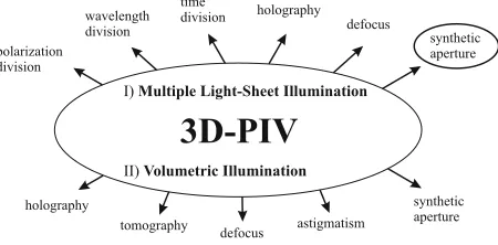
Particle image velocimetry (PIV) is nowadays one of the most common tools used in experimental flow studies, e.g. [1]. PIV provides two components of the flow velocity in two spatial dimensions in the measurement plane, which is generated by a light sheet. Comprehensive understanding of unsteady flow structures often requires velocity data not only in a single plane, but in multiple planes or in the complete 3D volume. Therefore, manifold techniques were developed extending the classical single-plane PIV to 3D space. In Fig. 1, we arrange in order the herein presented 3D-PIV technique to existing ones. After two decades of 3D-PIV developments two branches emerge: I) PIV by multiple light-sheet illumination and II) PIV by volumetric illumination. Another classification type may be the number of detectable spatial dimensions (short: D) and velocity components (short: C) [2], which is used subsidiary in this work.

Fig. 1Classification of 3D-PIV techniques by light-sheet and volumetric illumination. The encircled synthetic aperture PIV is introduced in the present work.

At least six physical quantities allow the separation of particle stray-light from different light sheets: polarization [3], wavelength [4,5], time [6], phase (holography) [7], size of defocus blur [8] and parallax (herein presented). Techniques using volumetric illumination are: holographic PIV [2], tomographic PIV [9], defocussing PIV [10], astigmatism PIV [11] and synthetic-aperture PIV [12].

Light-field imaging was introduced to fluid mechanics as synthetic-aperture particle image velocimetry (SAPIV) [12]. The name is retained in this work. Belden et al. use eight cameras mounted in an aluminum frame. All cameras image the same particle-laden flow. Recorded images are recombined by algorithms known from computer vision in order to obtain depth information, e.g. [13].

Especially for SAPIV large depth resolution is obtained in the expense of sensor size. As the parallax between adjacent views is essential for depth estimation, reducing the sensor size inevitably reduces depth resolution. Combining SAPIV with multiple light-sheet illumination enables downsizing to a single-camera setup, which is applied herein. Two components of the velocity field are measured by the sensor in multiple planes (3D2C), which already provides important spatial information of the flow in many applications. Separating the signals of different light-sheets is straight forward. No inverse multiplexing units are required (see e.g. [3–7]). Such a single-camera 3D-technique enables the observation of flows through narrow viewports and minimizes hardware complexity. The working principle of SAPIV in multiple measurement planes is explained in section 2. The generation of synthetic particle images for testing the SAPIV refocusing algorithm is presented in section 2.4. The validating experiment is illustrated in section 3. Results and Discussion are given in section 4, followed by Conclusions in section 5.

2 Method

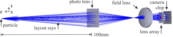
The principle of light-field imaging is to capture not only spatial coordinates of the intensity distribution on the sensor plane, but also angles of the light that forms the image [14]. This allows the reconstruction of 3D spatial information by refocusing on different planes. The first technologically relevant work on light-field imaging is by Adelson et al., who named their device a plenoptic camera [15]. Commercial plenoptic cameras using the Adelson-approach are available recently, see e.g. [16]. Beside this light-field technique there is another approach, the focused plenoptic camera [17]. The lens array images the focal plane of the photo lens, instead of focusing at infinity like in a traditional plenoptic camera. The first publication on light-field imaging in fluid mechanics is akin to it. It was named synthetic-aperture particle image velocimetry (SAPIV) [12]. The technique presented herein bases on the focused plenoptic approach. In the following we will focus on a single-camera solution with a planar sensor field, which is depicted in Fig. 2. Different viewing angles are realized by a lens array in front of the sensor plane. The imaging process is discussed in this section.

2.1 Refocusing

The basic principle of SAPIV with a lens array and a single camera is illustrated in Fig. 3. Two particles P1 and P2 at axial positions Z1 and Z2 are imaged through the planar lens array.

The numerical aperture of the lenses in our application is about NA=0.008. Therefore, the depth of field is large. Hence, both particles are imaged sharply. For illustration the particle P1

is colored green and P2 is colored black. In the following we discuss how the two different

particles are reconstructed out of the 2D image on the sensor plane.

Fig. 3.(Color online)Basic principal of synthetic-aperture imaging. Two differently colored particles are imaged though optics containing a lens array. Each lens images both particles

resulting in the given image.

When imaging P1 and P2 through the optics shown in Fig. 2, the magnification is different

for each particle due to different Z-positions. Each lens in the array images the particle pair at different angle, hence the magnification also depends on particle and lens position. This leads to the diverging dot pattern in Fig. 3. As the lens array is static, the variation of the dot pattern only depends on the particle position Z. The “image” in Fig. 3 consists of twenty-one sub-images corresponding to twenty-one lenses in the array. Image processing is used to refocus particle images on the different planes Z1 or Z2. The first step is the decomposition of the

image plane into sub-images, which each correspond to one lens of the array (Fig. 4). In order to refocus on position Z1 all sub-images are superposed such that the green dots finally overlie,

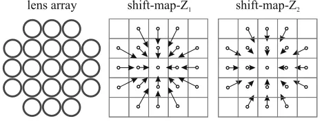
see step two in Fig. 5. Therefore, all sub-images are shifted appropriately against the central sub-image. Shifts are defined in a shift-map, Fig. 4. This procedure is repeated with another shift-map to refocus on plane Z2. Hence, different shift-maps refocus on different planes.

Fig. 4. Lens array and shift-maps containing shift-vectors h for matching particle images from different depths Z1 and Z2. The image plane is decomposed into sub-images for all lenses. One

shift-vector is used for one sub-image.

high-quality doublet lenses in the array, see section 2.4. For imaging at large field angles homographies with non-linear grids should be applied.

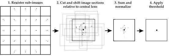
In step three, all shifted sub-images are summed up. Because of constructive summation of images of particles in the refocused plane, large peaks appear as in Fig. 5, where the peak belongs to particle P1 at position Z1. The evolved image is cropped to the dimensions of the

central sub-image and intensity is normalized. Finally, in step four, a threshold is applied to eliminate destructively summed gray-scale values, which belong to out-of-focus particles. Step two to four may be repeated with different shift-maps to refocus on different Z-positions. All steps of the refocusing algorithm are sketched in Fig. 5.

Fig. 5.Schematic of the four-step algorithm for refocusing images obtained by SAPIV.

2.2 Uncertainty of depth

To determine the uncertainty in depth, we consider two particles P1 and P2 at different depths.

This time they represent particles within a light sheet; one in the center, another one at the edge of the light sheet. Only if the images of P1 and P2 can be separated clearly, their depth

position can be determined uniquely. In Fig. 6, ray propagation is illustrated through lens b) of a lens array for an object height that equals the lens pitch p. The present case only considers a cross-section through the lens array. Meaning, image heights h1, h2 and pitch p are scalars.

Fig. 6. Imaging of particles P1 and P2 at different Z-position through lens b) along one line

through the lens array. The object height equals lens pitch p. Image heights are denoted by h1

and h2.

Both particles P1 and P2 are imaged at different magnification resulting in different image

point positions, spaced by ∆h = h1 – h2. As a necessary condition both particle images need to

be separated by at least one pixel edge length lpx, which requires ∆h ≥lpx. On the other hand,

the lower bound |∆h| = lpx determines the measurement uncertainty in depth. With a given

i i

-b -b h p

-Z Z Z

 

∆ =  

+ δ

  (1)

, where b denotes the image distance and Zi the central light-sheet location. The magnification

at light-sheet position Zi isβ =i -b / Zi. With the condition∆ = ±h lpx, distance δZ becomes the

uncertaintyδ = ±Z b 1/ (

[

]

for δZ reads:

i i

i

Z Z

1 /

β δ = ±

+ β γ (2)

As known from stereo imaging, uncertainty δΖ is inversely proportional to the detectable parallax [19], which is a determined by lens pitch p. With Eq. (2) andγ≪β, the following proportionality holdsδZ∼(FOV l ) / p⋅ px . Note that magnification β~1/FOV. Reducing the

pixel size of the used camera lpx could decrease δZ significantly. On the other hand, if the

FOV has to be enlarged without exchanging the optics, the light-sheet spacing ∆Z should be increased in order to retain high reconstruction quality.

As the real optics include further lenses along the optical axis (o.a.) like the field lens, the object distance Zi or image distance b cannot be measured directly. The uncertainty δZ is

determined experimentally by measuring the scale of magnification on adjacent measurement planes at Zi and Zi+1. Then, the image distance is calculated byb=-∆Z / [1 /βi-1 /βi 1+], with

∆Z the spacing between adjacent light-sheets.

Knowledge of δΖ is important, as it determines the maximum light-sheet thickness d and the minimum required light-sheet spacing ∆Ζ for unique depth measurements. The light-sheet thickness d is determined by the smallest feasible δΖ. It is calculated by largest βi and largest

pitch pmax,which equals the distance between the central and the outermost lens in the lens

array. Then, d should be chosend≤2 Zδ _min , which is typically in the order of a millimeter for flow applications. Otherwise, refocusing quality might be deteriorated by too many out-of-focus particles. The uncertainty δΖ is maximal for smallest βi and smallest pitch pmin, which

equals the distance between the central lens and its nearest neighbor. For optimum conditions, the light-sheet spacing should be∆ ≥Z 2 Zδ _max .

2.3 Calibration

In Fig. 6 the image heights h1 and h2 equal the x-dimension of shift-vectors h for different

depths Z, between the central lens and its nearest neighbor. Typical shift-vector maps are shown exemplarily in Fig. 4. Magnification β can be calculated analytically by laws of geometric optics. With effective focal length f, the conditional equation reads:

[

]

2 _{2 - (Z b) / f 1 0}

β + + β + = (3)

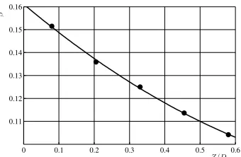
Fig. 7. Image magnification β as a function of depth Z, measured within a flow basin of D=100mm edge length. The fit-function reads β=0.054(Z/D)²-0.13Z/D+0.16.

The difference βi+1-βi is a measure for the capability of separating particles on adjacent light

sheets. The key task of sensor adjustment is its maximization. Eq. (3) is valid for perfect alignment of the lenses in the array, especially in absence of lens tilt. Following Fig. 6, shift-vectors can be calculated by h = βp. Here, p is the pitch vector. In practice, measured shifts will differ from theoretic values. Hence, it is inevitable to calibrate the sensor. Measured magnitudes of h for all present pitches |p| are given in Fig. 8.

Fig. 8. Measured shift magnitudes |h| for selected sub-images as a function of Z/D within a flow basin with an edge length of D=100mm. Four different curves corresponding to four

different lens pitches |p| (1-4) are displayed.

2.4 Optical simulation

The sensor´s ability to reconstruct the particle positions in 3D is simulated by synthetic particle images and ray tracing. Therefore, the SAPIV optics is implemented in the simulation code ZEMAX. Reconstruction quality is analyzed as a function of the applied refocusing threshold and the seeding density.

In ZEMAX the photo lens is modeled as paraxial plane to account for its high-quality imaging characteristics. The field lens and the lens array are modeled by original glass, radii and thickness data. The implemented setup is identical to the experimental one in section 3.1. The layout is given in Fig. 2. Tracer particles are modeled by plane, circular surfaces, 100µm in diameter, which emit Gaussian-shaped light. Ray tracing is conducted using ZEMAX´s non-sequential mode. The number of analysis ray for coherent ray tracing is 3e5. Rays originate at the particle position and hit the 1024x1024 pixel detector (sensor chip).

A real measurement situation is simulated by particles distributed randomly on five equally spaced XY-planes. These planes correspond to the light sheets used in practice. Intensity fields are calculated and exported for each Z-position. Later on, the five exported intensity fields are compared directly to refocused images.

0 0.1 0.2 0.3 0.4 0.5 0.6 0.11

0.12 0.13 0.14 0.15 0.16

Z/D

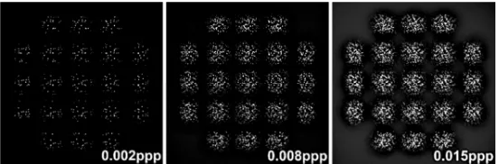
The detector image is then the sum of intensity fields of all illuminated particles in the measurement volume. This image is refocused using the SAPIV algorithm described in section 2.1. Refocusing on the Z-positions that were preset in ZEMAX should result in images similar to the previously exported intensity fields. Any deviations between exact and refocused images are due to reconstruction errors. Naturally, these errors deteriorate reconstruction quality. Simulated intensity fields generated at three different seeding densities are shown in Fig. 9. The images are generated by 10, 50 and 100 randomly distributed particles on each of the five Z-planes. Particle densities on the detector are 0.002, 0.008 and 0.015 particles per pixel (ppp). The 1/e²-diameter of a particle is 2px. The particle density is determined by the number of all particles on the detector divided by the detector area in pixel.

Fig. 9. Simulated intensity fields generated by the SAPIV optics at 0.002, 0.008, 0.015 particles per pixel (ppp). Particles are randomly distributed on five equidistant measurement planes,

imaged by the optics shown in Fig. 2.

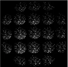
Refocusing of the images given in Fig. 9 is carried out by means of the shift maps, like that shown in Fig. 4. The shift map for each depth Z is determined by calibration. Therefore, a single particle at X=0, Y=0 is imaged. A cross-correlation procedure between all sub-images and the central sub-image then provides the shift maps, see section 2.3. Sub-images in the recordings are interpolated using a grid of 0.1px step size, which allows shifting at a precision of 0.1px. From the mid image in Fig. 9, the central sub-image is depicted magnified in Fig. 10, left. Refocused images of five different measurement planes are merged into one color-coded illustration, Fig. 10, right.

Fig. 10. (Color online) Comparison of raw (left) and refocused (right) particle images at 0.008ppp seeding density. Depth Z is color-coded.

Obviously, darker particles at the rim of the raw image are not reconstructed. They are much darker than the brightest particles. Decreasing the threshold value increases the effective field of view (FOV). However, this will deteriorate the reconstruction quality.

2.4.1 Reconstruction quality

Q>0.75 [9]. The same argument is used here to estimate the maximum seeding density up to which correlation-based velocimetry will work with the presented light-field camera.

(

)

i

i

r i 0 i

X,Y,Z

2 2

r i 0 i

X,Y,Z X,Y,Z

I X, Y, Z I (X, Y, Z ) Q

I (X, Y, Z ) I (X, Y, Z )

⋅ =

⋅

∑

∑

∑

As described in section 2.1, refocused images are obtained by applying a threshold to the sum of the twenty-one shifted sub-images. In Fig. 11, the reconstruction quality Q is plotted as a function of the threshold in gray-scale values and the seeding density in ppp.

Fig. 11. Reconstruction quality Q as a function of the refocus-threshold in gray-scale values and the seeding density in particles per pixel (ppp).

The displayed set of curves is Gaussian, as the histogram of refocused and original intensity field, Ir and I0, is Gaussian as well. Beside the maxima of the curves the average change in

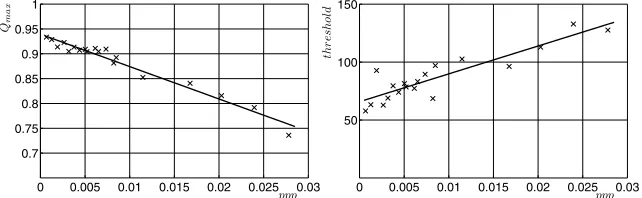
reconstruction quality is ∆Q / threshold∆ ≈ −0.004. In first approximation, the maximum reconstruction quality Qmax decreases linearly with increasing seeding density, which is

illustrated in Fig. 12, left. A linear fit is applied and plotted as solid line. If you assume Q=0.75 as minimum acceptable reconstruction quality [9], the maximal seeding density is about 0.03ppp.

Fig. 12. Maximum reachable reconstruction quality Q (left) and corresponding threshold in gray-scale values as a function of the seeding density in particles per pixel (ppp). The linear

trends (solid lines) are: Qmax=0.94-6.5ppp and threshold=65.8+2400ppp.

The required threshold to achieve a maximum of Q is a function of the seeding density. The relation is given in Fig. 12, right. The linear trend helps to estimate optimum thresholds for refocusing. Required thresholds increase for increasing particle density.

all measurement planes. The overall uncertainty isσ =_r (rms2_X+rms )2_Y 1/ 2. Values of σr at

largest reconstruction quality Qmax are plotted in Fig. 13 over the seeding density. At seeding

densities larger than 0.005ppp particle images overlap more and more and the calculation of centroid positions fails. For this reason large seeding densities are not possible in PTV, the upper limit is about 0.005ppp [20], see Fig. 13.

Fig. 13. Root mean square deviation σr between exact and refocused positions of particles

present in the measurement volume. The linear trend (solid lines) is: σr=0.14+28.8ppp.

3 Experiment

3.1 Sensor Setup

Fig. 14.Experimental setup for single-camera SAPIV. The illuminating laser beam is expanded to five light sheets by an optical grating. The receiving optics is aligned normal to the light sheets. Tracer particles from all light sheets are imaged onto the sensor plane at the same time.

The complete optics is sketched in Fig. 14. Illuminating optics and flow basin are mounted on an aluminum frame. Their orientation is illustrated in Fig. 14. The laser is a Minilite (Continuum, USA) with 5ns pulse width and 5mJ pulse energy is used for experiments. The repetition rate of the laser is 1Hz, forced by an external trigger. The 2mm laser beam is expanded to a sheet by a negative cylindrical lens (focal length f=-25mm). Subsequently, the beam propagates a phase grating. In a distance of about 300mm behind the grating five diffraction orders are parallelized by a cylindrical lens, f=300mm. After parallelization the

0 0.001 0.002 0.003 0.004 0.005 0.006

0.1 0.2 0.3 0.4

ppp

σr

[

px

light sheets are equally spaced by ∆Z=12.5mm. The grating exhibits nearly the same intensity distribution in the +1st, 0 and –1st diffraction order. In the +2nd and –2nd order the diffracted intensity is lower. Applying neutral density filters for the inner three orders equalizes light intensity in all light sheets. This is important as inhomogeneous sheet intensities could disturb the reconstruction quality.

The receiving optics and the camera are mounted on a rail allowing on-axis shifting relatively to the flow basin. The front lens is a photo lens, focal length f=50mm with a free aperture diameter of D=30mm, located at a distance of 100mm to the nearest light sheet. The photo lens can be zoomed in and out, which allows controlling the working distance without changing the alignment of the optics. The field lens is a singlet lens with f=50mm, D=28mm. The lens array consists of twenty-one doublet lenses (Edmund Optics) with f=9mm, D=2mm. The doublets are aligned in a quadratic grid and glued into a frame consisting of two identical silicon plates by polydimethylsiloxane (PDMS). The outer edges of the square array are left free, as imaging quality would be insufficient for lenses located there. 2mm holes are etched into both silicon plates as apertures. The lens pitch between adjacent lenses is 3.13mm. The distance between photo and field lens is 90mm, between field lens and lens array it is 30mm. The intermediate image is a demagnified version of the flow. At its position an aperture plate with variable diameter enables fine adjusting the final size of the measurement volume. It prevents sub-images from overlapping and blocks large field angles, which minimizes distortion aberration. The aperture plate, field lens and the lens array and are mounted in a LINOS micro bench. As we apply a simple homography for refocusing (see section 2.1) the lens array should provide superior imaging characteristics. Doublet lenses exhibit considerably less wave-front aberration compared to singlet lenses [21]. The used camera is a Photron APX RS 1024x1024px with a CMOS chip, 17.8x17.8mm² in size and 17.4µm pixel edge length. The camera is triggered by the same electronics determining the repetition rate of the laser.

Applying Eq. (2) with minimum pitch, p=3.13mm, and minimum magnification (see Fig. 7) yieldsδZ_max = ±6mm. Therefore, the optimum light-sheet spacing should be larger than 12mm. The optical simulation in section 2.4.1 reveals sufficiently high Q for ∆Z=12.5mm. Applying the maximum occurring pitch in the used lens array, p= 5 3.13mm⋅ (see Fig. 8), and maximum magnification yields δZ_min = ±2mm. Consequently, the light-sheet thickness d should be smaller than 4mm for high reconstruction quality. In practice, it is d=1.5mm, which is advantageous for highly seeded flows, as only a fraction of the seeding is imaged onto the camera chip.

The field of view (FOV) is imaged multiplied onto the CMOS chip by the lens array. In the present case the effective chip area used to capture the FOV is 204x204px. The active chip area is given by the number of lenses in the array. Magnification β is significantly different for each light sheet. Knowledge of the exact value of β is required for determination of lateral particle positions on individual light sheets.

3.2 Calibration

sub-image. Shifts are determined at positions of the five light sheets and connected by straight lines. The maximal measured shift is 72px, the smallest one is 17px. The sensor´s depth sensitivity is given by the gradient of the shift function.

3.3 Convective flow

For validation single-camera SAPIV is applied to a three-dimensional convective flow. The fluid is heated laterally, which is a relevant configuration for the manufacture of bulk semi-conductor crystals, see i.e. [22]. The flow is generated in a basin with D=100mm edge length. One side wall of the basin is connected to the heating, the opposite wall to the cooling circuit, see Fig. 17. Both circuits are realized by independently working water thermostats (Julabo HC, Germany). The remaining four walls of the flow basin are adiabatic. Adiabatic walls are made from PMMA and therefore are transparent. The temperature controlled walls are made from aluminum. Thermo couples log the wall temperature during measurements. In thermodynamic equilibrium, the temperature controlled walls exhibit mean temperatures of 76.88°C and 5.86°C respectively.

The basin is filled completely by a 0.73:0.27 water-glycerin solution resulting in 1.061g/cm3 fluid density at 30°C (Glycerine Producers' Association, 1963). Glycerin is added to the fluid in order to adapt the fluid´s density to the used tracer particles. Tracers are made from polyamide 12 base polymer (Vestosint 1141, Evonik, Germany). The fraction of 55 % of particles ranges from 100µm to 250µm in diameter. The realized particle density is 0.007 particles per pixel (ppp), which equals 0.06 particles per mm³ in the illuminated measurement volume. After reaching thermodynamic equilibrium the recording is started at 1Hz repetition rate of laser firing and camera exposure. 2048 images are recorded. In Fig. 15 a 1024x1024px snapshot of particles present on all five light sheets is displayed.

Fig. 15. 1024x1024px snapshot of tracer particles in the flow basin. The image is formed by twenty-one single lenses. Tracer particles are distributed in depth on five light sheets equally

spaced by 12.5mm. The diameter of the field of view is about 30mm.

Fig. 16. Process chain of refocusing tracer particles. The refocused plane is at Z/D=0.46. Left: Unprocessed 204x204px central sub-image. Mid: Normalized sum of 21 shifted sub-images.

Right: Refocused imaged, generated by applying a threshold.

4 Results and Discussion

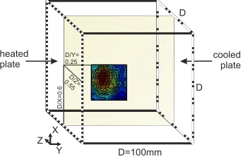
The process chain indicated in Fig. 16 is repeated for each light-sheet Z-position. Due to low seeding density a complete velocity field is computed by averaging 2048 recordings. Particle displacements are evaluated by the open source code fluere by K. P. Lynch on sequenced image pairs. The magnification scale is adapted for each light sheet in accordance to Fig. 7. A three pass algorithm is applied starting at 64x64px, continuing with 32x32px and ending at 16x16px interrogation window size. Windows are weighted uniformly. 50% overlap leads to a smallest window size of 8x8px, which determines the spatial resolution of the vector field to a minimum of 1.3mm edge length. Depth resolution is given by the light-sheet thickness of 1.5mm. Velocity vectors are validated in MATLAB using the ratio of the two largest correlation peaks. 2D Cross-correlation is applied for each Z-position separately. All validated two-component vectors are averaged over time. The orientation of the measurement volume within the flow basin is given in Fig. 17. Dimensions are related to the edge length D=100mm of the flow basin. As already mentioned, the measurement volume is composed of five XY-planes. The first one is at Z/D=0.08, the last one Z/D=0.58. All slices are spaced by Z/D=0.125. The lateral extension of measurement planes increases for larger values Z/D, as image magnification decreases.

Fig. 17. Orientation of the measurement plane at Z/D=0.58 within the flow basin. The heated plate is bordered dotted, the cooled one bordered dash-dotted.

The mean velocity field vabs is displayed in Fig. 18. It is composed of five XY-slices at five

Fig. 18. (Color online) Left: Section of temporally averaged, 3D velocity field in a laterally heated convective flow, determined by single-camera SAPIV. Five equally spaced light sheets between0.08 Z / D≤ ≤0.58are used for illumination. The hot wall is at Y/D=0, the cold wall at Y/D=1. Two-component velocity vectors are depicted as black vector-cones. The mean absolute velocity is given color-coded on XY-slices bordering the measurement volume. Right: Maximum average velocity on each measurement plane.

Single XY-slices are displayed in Fig. 19. The flow is directed upwards. As expected, the flow accelerates along X because of buoyant forces acting on the fluid. The flow seems to exhibit a single-roll pattern, whose center of rotation is underneath the center of the basin.

Fig. 19. Velocity fields on five measurement planes from Z/D=0.08 to Z/D=0.58 (from left to right), spaced by Z/D=0.125. Vectors point the direction of the flow in the XY-plane. For

velocity magnitudes see Fig. 18, right.

5 Conclusions

For correlation-based velocimetry high in-plane spatial resolution is required. As the presented light-field camera utilizes the focused plenoptic principle, the full image resolution of the applied CMOS-chip can be used. In commercial plenoptic cameras image resolution may be reduced due to the formation of macro-pixels; see [15]. Especially in applications using cameras with large pixels (e.g. high-speed imaging) the proposed optics is superior. The realized in-plane resolution is at least 80µm.

In fluid mechanics, up-to-now light-field imaging was realized with bulky setups by multiple cameras, see synthetic-aperture particle image velocimetry (SAPIV) [12]. In contrast to this, a single-camera 3D-PIV technique utilizing light-field imaging is presented. The technique allows two-component velocity measurements on multiple planes quasi-simultaneously (2C3D velocimetry). A lens array consisting of doublet lenses enables twenty-one views on a particle-laden flow at different angles. Simulations reveal that a reconstruction quality [9] of Q>0.75 is realistic for the present optics at seeding densities smaller than 0.03 particles per pixel (ppp). Compared to literature, reconstructed particle fields can be correlated at high quality.

views (FOV) are feasible at larger light-sheet spacing or by a camera with smaller pixel size. As SAPIV is a threshold technique, knowledge of the threshold scaling in dependence of the seeding density is fundamental. An optimal threshold is found by optical simulations.

In a validation experiment a seeding density of 0.007ppp is realized. This is low compared to existing 3D-PIV techniques [20] and reasoned by a maximum parallax of 1°. For instance, in tomographic PIV the angle of choice is typically 30° [9]. The working distance of the sensor can be varied easily by a zoom photo lens. No fine tuning is required between lens array and camera chip. Therefore, the technique is robust and easy to implement in the lab.

Single-camera, multiple-plane SAPIV is especially suited to environments not accessible for multiple-camera setups, like reactors or engines.

Acknowledgement