Methods and Tools for the
Microsimulation of Household
Expenditure
Tony Lawson
A Thesis Submitted for the Degree of Ph.D. Department of Sociology
Spending by households represents a significant component in the UK economy and the ability to model the effects of socio-economic change on household expenditure is crucial at both the commercial and governmental level. This is usually done by estimating the parameters of a demand system. However, there are several difficulties associated with this approach including, representing the heterogeneity of economic units, the dimensionality of a complex budget set and the specification of the
functional form. One way to avoid these is to develop a model that directly simulates the individual units in what is known as a microsimulation. However, models of this type have been found to be complex and expensive to develop. This thesis
Methods and Tools for the Microsimulation of Household Expenditure...1
Chapter 1: Introduction...1
1.1 Overview...1
1.2 Microsimulation Modelling...2
1.3 Expenditure Modelling...5
1.4 Research Questions...10
1.5 Methods...12
1.6 Structure of the Thesis...15
1.7 Conclusion...18
Chapter 2: Micro-level Modelling...20
2.1 Introduction...20
2.2 Modelling and Simulation...20
2.3 Microsimulation...23
2.3.1 Traffic Microsimulation...23
2.3.2 Spatial Microsimulation...24
2.3.3 Static Microsimulation...25
2.3.3.1 Arithmetical Microsimulation...25
2.3.3.2 Behavioural Microsimulation...26
2.3.4 Dynamic Microsimulation...27
2.3.4.1 Static Ageing...27
2.3.4.2 Dynamic Ageing...28
2.3.4.3 Alignment...32
2.4 Applications of Dynamic Microsimulation Modelling...34
2.5 Microsimulation Models of Consumption and Expenditure...38
2.6 Software for Microsimulation Modelling...42
2.6.1 UMDBS...44
2.6.2 LIAM...44
2.6.3 Modgen...45
2.7 Challenges for Microsimulation Modelling...46
2.8 Agent-based Modelling...49
2.8.1 Origins of ABM...49
2.8.2 Behavioural Representation in ABM ...52
2.8.3 ABM and Economics...54
2.8.4 ABM Software...54
2.8.4.1 Evaluation of Agent-based Modelling Toolkits...59
2.8.4.2 Review of NetLogo...62
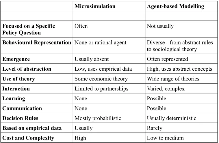
2.9 Microsimulation and Agent-Based Modelling...65
2.10 Evaluation of the Project...69
2.11 Conclusion...72
Chapter 3: Expenditure Modelling...73
3.1 Introduction...73
3.2 Time-series Models...73
3.3 Regression Methods...76
3.4 Demand Systems...78
3.5 Random Assignment...91
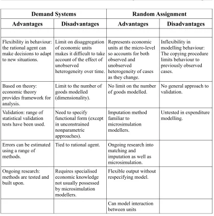
3.6 Advantages and Disadvantages of Demand Systems and Random Assignment in Microsimulation Modelling...95
4.1 Introduction...99
4.2 Design Overview...100
4.3 Base Survey Data...102
4.4 Obtaining Transition Probabilities...103
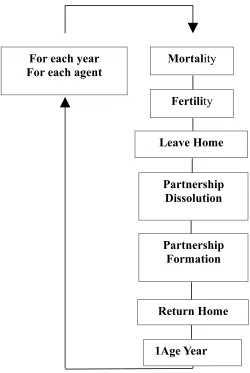
4.5 Operation of the model...107
4.5.1 Loading the Base Data...107
4.5.2 Mortality...108
4.5.3 Birth...110
4.5.4 Leaving the Parental Home...112
4.5.5 Marriage dissolution...113
4.5.6 Cohabitation dissolution...116
4.5.7 Cohabitation formation...116
4.5.8 Marriage formation...119
4.5.9 Age 1 Year...121
4.5.10 Returning home after separation...122
4.5.11 Locating children...122
4.5.12 Alignment...123
4.5.13 Summary of Transition Probability Determination...123
4.6 Validation and Verification...125
4.6.1 Sources of error...126
4.6.1.1 Measurement error...126
4.6.1.2 Sampling Variation...127
4.6.1.3 Static Parameters...127
4.6.1.4 Limited Number of Parameters...128
4.6.1.5 Stochastic Variation...128
4.6.1.6 Programmer Errors...129
4.6.1.7 Demographic Specification...129
4.6.2 Validation Scheme...130
4.6.2.1 Data / Coefficient / Parameter Validation...132
4.6.2.2 Programmer’s / Algorithmic Validation...132
4.6.2.3 Module-specific Validation...133
4.6.2.4 Multi-module Validation...133
4.6.2.5 Individual Output...134
4.6.2.6 BHPS Cross-sectional Validation...137
4.6.2.7 BHPS Longitudinal Validation...137
4.6.2.8 BHPS Individual-Level Projections...138
4.6.2.9 Household Level Projections...141
4.6.2.10 ONS Cross-sectional Validation...143
4.6.2.11 Alignment...144
4.6.2.12 Impact Validation...147
4.7 Comments on the Validation...147
4.8 Projected Demographic Change...149
4.9 Limitations and Further Work...153
4.10 Comparison with LIAM 2...154
4.10.1 Processing Speed Comparison...157
4.10.2 Usability and Flexibility...160
4.10.3 Discussion of the Results...162
4.11 Conclusion...163
5.2 Random Assignment...166
5.3 An Application of Random Assignment to Model the Effect of Changes in Income on Household Expenditure Patterns...170
5.3.1 Level of analysis...170
5.3.2 Data Source...171
5.3.3 Implementation...172
5.3.4 Matching Criteria...173
5.3.5. Running the Model...177
5.3.6 Validation...177
5.3.6.1 Theoretical Validation...181
5.3.6.2 Reproduction of a Known Relationship...182
5.3.6.3 Stylised Facts...185
5.4. Results...186
5.4.1. Average Spending...186
5.4.2 Older Households and Families with Young Children...190
5.4.3. Analysis by Income Quintile...192
5.5 Discussion...193
5.6 Conclusion...195
Chapter 6: Demographic Change and Expenditure ...197
6.1 Introduction...197
6.2 Demographic Change and the Ageing Population...199
6.3 Combined Demographic/Expenditure Model...200
6.3.1 Expenditure Model Specification...201
6.3.2 Alignment...202
6.3.3 Running the Model...203
6.4 Results...205
6.4.1 Changes in Household Income...206
6.4.2 Spending Patterns Over the Life-course...207
6.4.3 Projection of Household Expenditure...208
6.4.4 Impact Validation...218
6.4.4.1 Totals Check...218
6.4.4.2 Comparison with Previous Results...221
6.4.4.3 Sensitivity Analysis...222
6.5 Disaggregated Results...224
6.5.1 Spending by Age Band...224
6.6 Spending by Industrial Sector...228
6.6.1 Spending by Age Band...229
6.6.2 Spending by Household Type...234
6.7 Alternative Economic Scenarios...240
6.7.1 Detailed Analysis of Scenario 2...244
6.8 Discussion...248
6.8.1 Comments on the results...249
6.8.2 Comments on the Method...257
6.9 Conclusion...260
Chapter 7: Further Applications...263
7.1 Introduction...263
7.2 Scenario 1: The Effect of Energy Prices on Household Spending...265
7.2.1 Energy Price Change Model...266
7.3 Scenario 2: The Effect of a Shift Towards Homeworking...279
7.3.1 Data Source...283
7.3.2 Results...291
7.3.3 Discussion...293
7.4 Conclusions and Further Work...294
Chapter 8: Conclusion...296
8.1 Introduction...296
8.2 Responses to the Specific Questions...299
8.3 The General Questions...304
8.4 The Main Question...305
8.5 Contribution to Knowledge...306
8.6 Impact on Microsimulation...309
8.7 Further Work...311
8.8 Conclusion...313
Figure 1: Distribution of UK Household Spending...6
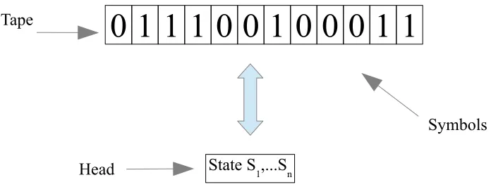
Figure 2: Schematic Representation of a Turing Machine...50
Figure 3: Turing Machine State Transition Diagram...50
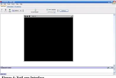
Figure 4: NetLogo Interface...63
Figure 5: Microsimulation Modules...101
Figure 6: Risk of Death by Age (ONS)...109
Figure 7: Number in Household Compared Against BHPS 2008...137
Figure 8: Marital Status (married, divorced, widowed)...139
Figure 9: Marital Status (single, cohabiting, separated)...140
Figure 10: Age Bands...141
Figure 11: Household Types (single non-pensioners, single pensioners, couples)....143
Figure 12: Household Types (family, single parent, other)...143
Figure 13: Projected Age Distribution of UK Population in 2031...144
Figure 14: ONS and Model Projected Birth Rates...145
Figure 15: ONS and Model Projected Death Rates...146
Figure 16: Change in UK Population...150
Figure 17: Number of UK Households...151
Figure 18: Age Distribution of Households...151
Figure 19: Household Occupancy 2006 to 2036...152
Figure 20: Time to Load and Process 1 Simulated Year...158
Figure 21: LIAM2 User Interface...160
Figure 22: Tyche User Interface...161
Figure 23: NetLogo GUI Features...162
Figure 24: Results from modelling artificial rule...183
Figure 25: Modelling an Artificial Rule with Random Disturbances...185
Figure 26: Share of Expenditure (older households and families with young children) ...191
Figure 27: Share of Expenditure by Quintile...193
Figure 28: Combined Model User Interface...203
Figure 29: Endogenous Change in Average Household Income: 2006 - 2036...206
Figure 30: Endogenous Change in Aggregate UK Total Household Income...207
Figure 31: Spending Patterns for Different Age Groups in 2006...208
Figure 32: Total Expenditure...211
Figure 33: Food (food & non-alcoholic drinks)...211
Figure 34: Alcohol (alcoholic drinks, tobacco & narcotics)...212
Figure 35: Clothing (clothing & footwear)...212
Figure 36: Housing (housing, fuel & power)...212
Figure 37: Furniture (household goods & services)...213
Figure 38: Health...213
Figure 39: Transport...214
Figure 40: Communication...214
Figure 41: Recreation (recreation & culture)...215
Figure 42: Education...215
Figure 43: Hotels (restaurants & hotels)...216
Figure 44: Miscellaneous (miscellaneous goods & services)...216
Figure 45: Effect of Alternative Transition Probabilities...223
Figure 46: Expenditure by Age Band (housing, health, transport, food)...226
Figure 47: Aggregate Spending on Housing by Age Band...227
Figure 50: Aggregate Spending on Food by Age Band...228
Figure 51: Share of Food Spending by Age Band...229
Figure 52: Share of Alcohol Spending by Age Band...230
Figure 53: Share of Clothing Spending by Age Band...230
Figure 54: Share of Housing Spending by Age Band...231
Figure 55: Share of Furniture Spending by Age Band...231
Figure 56: Share of Transport Spending by Age Band...232
Figure 57: Share of Communication Spending by Age Band...232
Figure 58: Share of Recreation Spending by Age Band...233
Figure 59: Share of Education Spending by Age Band...233
Figure 60: Share of Hotels Spending by Age Band...234
Figure 61: Share of Food Spending by Household Type...234
Figure 62: Share of Alcohol Spending by Household Type...235
Figure 63: Share of Clothing Spending by Household Type...235
Figure 64: Share of Furniture Spending by Household Type...236
Figure 65: Share of Health Spending by Household Type...236
Figure 66: Share of Transport Spending by Household Type...237
Figure 67: Share of Communication Spending by Household Type...237
Figure 68: Share of Recreation Spending by Household Type...238
Figure 69: Share of Education Spending by Household Type...238
Figure 70: Share of Hotels Spending by Household Type...239
Figure 71: Share of Miscellaneous Spending by Household Type...239
Figure 72: Expenditures and Budget Shares at the Start of the Simulation...271
Figure 73: Expenditures and Budget Shares after 1 Year...272
Figure 74: Expenditures and Budget Shares after Rescaling...273
Figure 75: Changes in Expenditure due to a 10% Annual Increase in Energy Prices ...275
Figure 76: Changes Expenditures when 'Other' Costs are Fixed (£ per week)...277
Table 1: Summary of Microsimulation and Agent-based Modelling Characteristics..67
Table 2: Advantages and Disadvantages of Modelling Approaches...96
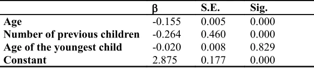
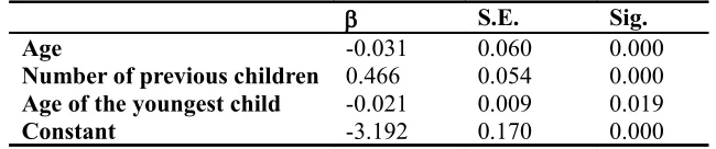
Table 3: Parameter estimates of whether a married woman gives birth in the current year...110
Table 4: Parameter estimates of whether a cohabiting woman gives birth in the current year...111
Table 5: Parameter estimates of whether an unpartnered woman gives birth in the current year...111
Table 6: Probability of multiple births by age of mother...112
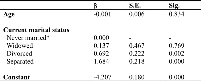
Table 7: Parameter estimates of marriage dissolution for males...115
Table 8: Parameter estimates of marriage dissolution for females...115
Table 9: Parameter estimates of cohabitation dissolution for males...116
Table 10: Parameter estimates of cohabitation dissolution for females...116
Table 11: Parameter estimates of a male beginning cohabiting in the next year...117
Table 12: Parameter estimates of a female beginning cohabiting in the next year....117
Table 13: Parameter estimates of whether a cohabiting male will marry his cohabitee in the current year...120
Table 14: Parameter estimates of whether a cohabiting female will marry her cohabitee in the current year...120
Table 15: Parameter estimates of whether a non-cohabiting male will marry in the current year...121
Table 16: Parameter estimates of whether a non-cohabiting female will marry in the current year...121
Table 17: Summary of Transition Probability Determination...124
Table 18: Individual Output...136
Table 19: Shapiro-Wilk Test for Normality...139
Table 20: Functionality of Tyche and LIAM2...156
Table 21: Initial Dataset...166
Table 22: Donor Case Assignment...167
Table 23: Completed Income Projection...168
Table 24: Primary EFS Expenditure Categories...172
Table 25: Ten households which spend spend 10% of their income on a good ...182
Table 26: Input Data with Stochastic Disturbance...184
Table 27: Shapiro-Wilk Test for Normality...188
Table 28: Share of Expenditure with Increasing Income (all households)...189
Table 29: Analysis of Distribution of Total Expenditure over 10 Simulations...210
Table 30: Normalised Aggregate Expenditure...217
Table 31: Budget Shares (%)...217
Table 32: Aggregate Expenditure Change 2006 - 2036 in Four Scenarios...243
Table 33: Change in Budget Share 2006 to 2036 in Four Scenarios...244
Table 34: Changes in Spending for Food between 2006 and 2036...246
Table 35: Food Expenditure 2006...247
Table 36: Food Expenditure 2036...248
Table 37: Sensitivity of Categories of Household Good to the Price of Energy...268
Table 38: Change in Expenditures (£ per week)...274
Table 39: Change in Expenditures when 'Other' Costs are Fixed (£ per week)...276
Table 40: Household Level Variables...284
Chapter 1: Introduction
1.1 Overview
For governments, the ability to anticipate how consumer spending is affected by economic conditions, demographic change or its own policy initiatives, is a key component in managing the economy. Also, for commercial organisations, projecting changes in the level of demand for their goods and services, in a changing world, can make the difference between success and failure.
This is usually done using econometric methods that involve estimating the
parameters of an equation that links spending patterns with a set of variables that are thought to influence spending behaviour (Clements and Hendry, 2002). However, as this thesis argues, the econometric approach is limited in its ability to allow for the way that the differences between individual cases affect the way spending patterns change in response to varying socio-economic conditions. One solution is to develop a model that directly simulates the individual units in what is known as a
microsimulation, as proposed by Orcutt (1957). The aim of this research is to develop a conceptual and technical framework for the microsimulation of household
expenditure and then show how it can be used to model the effect of socio-economic factors on household spending patterns.
new combinations of methods and tools by constructing and evaluating
microsimulation models of how household expenditure patterns are affected by income and demographic change.
This introduction begins with an overview: first of microsimulation modelling and then expenditure analysis. In each case it identifies problems or difficulties with current methods and these provide the motivation and justification for this research. This leads on to a definition of the research questions that the thesis is intended to answer. The chapter concludes by outlining the structure of the main body of the thesis.
1.2 Microsimulation Modelling
Microsimulation (Orcutt, 1957) was conceived to solve a general problem in macro-economic modelling, which was that the aggregated variables used to represent the parameters of an economic system do not correctly represent the distribution of those parameters as measured at the level of individual decision making units. Orcutt illustrated this with a numerical example where there is a set of individuals which are imagined to have input X and output Y as shown in the table below.
X Y
0 0
1 1
2 1
of 1, will generate an output of 100. It is also apparent that if the population is made up of 50 individuals with an input of 0, and another 50 with an input of 2, the combined input will still be 100 as before but the sum of the output will now be 50. Thus, knowledge of inputs at the macro-level does not uniquely determine the output of the system as a whole. Orcutt proposed to solve this problem with a model that preserves the micro-level characteristics of the individual elements. This takes the form of a simulation composed of ‘interacting units’ which receive inputs and generate outputs. The inputs he defines as anything which acts upon, or is taken account of, by the unit. These could be things like age, income or the rate of inflation. They could also be the outputs from other microsimulation units. Outputs are
anything which stems from, or is generated by the unit. Examples of outputs include marriage or the birth of a child. The heart of the unit that generates outputs from inputs is what Orcutt calls the ‘operating characteristics’. These can be implemented in a variety of ways including equations, graphs or tables.
implementations (Spielauer, 2007). These include MOSART in Norway, developed to model public expenditure (Fredriksen, 1998) and DESTINIE in France, to project pension requirements (INSEE, 1999). In the UK, a range of models has been
developed to assist in policy formation. These include PENSIM, which has been used in pension forecasting (Hancock et al., 1992), CARESIM for anticipating demand for healthcare (Zaidi and Rake, 2001) and SAGE (Simulating Social Policy in an Ageing Society) (Cheesbrough and Scott, 2003) which simulates the effects of demographic change on demand for pensions and healthcare.
Currently, there are several varieties of microsimulation in use (O’Donoghue, 2001a), (Li and O'Donoghue, 2013) but in general they can be divided into two main types: static and dynamic (Merz, 1993). In a static microsimulation, the unit generates a set of outputs from a set of inputs but is not itself changed in the process. In a dynamic microsimulation the unit changes or ‘ages’ over time. This makes dynamic
microsimulation useful for modelling long-term processes such as demographic change. This thesis is primarily concerned with dynamic microsimulation.
By the late 1990s, microsimulation was making a contribution to informing
microsimulation model already built in, such as mechanisms to handle the collection of agents and an advanced graphical user interface (GUI). As such, they might well have the potential to reduce the complexity of developing the model. While there are already some examples of microsimulation models developed using an ABM platform such as LaborSim (Leombruni and Richiardi, 2005) and IFSIM (Baroni, Zamac and Oberg, 2009), these have all been of a type that utilises a general-purpose
programming language and this still requires advanced programming skills on the part of the developer. There has been no attempt to apply a simpler, script-based ABM platform. One of the objectives of this research will be to investigate the extent to which one of these toolkits, known as NetLogo, can reduce the burden of developing a dynamic microsimulation model. This will be done by implementing one such model using NetLogo and evaluating its performance in terms of its ability to implement all the necessary functions, its processing speed and usability. The resulting dynamic microsimulation model, known as Tyche, will then be combined with an expenditure component and applied to model household spending patterns.
1.3 Expenditure Modelling
These figures, taken from the 2006 EFS, relate to consumption expenditure which can be thought of as spending on things to use rather than sell or trade. Commercial organisations operate in one or more of these sectors and the share of household expenditure devoted to each one gives an indication of the size of the market for a particular good or service. Market size is known for the current and previous years but it is desirable to have some understanding of the factors that influence spending and then to project it into the future. This might assist, for example, in an
[image:17.595.94.461.109.354.2]organisation’s strategic planning. If a market is projected to grow then it might be worth expanding activities in that area or investing in new technology. If the sector seems likely to decline then it may be advisable to consolidate or perhaps look to another sector.
Figure 1: Distribution of UK Household Spending Food
12%
Alcohol & tobacco 3%
Clothing & footwear 6%
Housing water & electricity 13%
Furnishings & hh equipment 8%
Health
2% Transport
16%
Communication 3%
Recreation 15% Education 2%
Restaurants & hotels 10%
Governments obtain revenue from taxation and this affects how much households have remaining to spend on consumption items. This is particularly relevant in the case of indirect taxes where the level of taxation on a particular item can affect how much of it is consumed and as a consequence, affect the amount of revenue
generated.
The importance of analysing spending patterns for such a wide range of organisations has led to the development and application of a formidable array of methods. These range from approaches that rely on the knowledge and judgement of individuals to complex mathematical models. Some are essentially macro methods in that they model aggregated variables and the relationship between them. When modelling expenditure patterns at the level of individual households, the dominant approach is to use econometric methods (Clements and Hendry, 2002). It is possible to do this in a single, regression type equation of the form:
Y=b0b1X1b2X2...bnXn
Here, the dependent variable Y might represent the budget share for food. The
independent variables X1 to Xn could represent factors that are thought to influence spending on food such as household size, income and price. The constants
b0 to bn would be estimated using standard statistical software on observed data
that captures the relationship between the relevant variables.
large as it would be in a typical household budget set. It is also difficult to model the interaction between spending on each good because, in principle, this will depend on what is spent on all the other goods. The list of independent variables should then include the budget shares of all these items. This is feasible for a small number of goods but as the size of the budget set increases, the number of parameters needed to estimate the model grows quickly to the point where, for most datasets, there would not be enough cases to provide accurate estimates of the parameters.
This problem is alleviated to some extent by the use of complete demand systems consisting of an integrated set of equations. Some of the most sophisticated are the Quadratic Almost Ideal Demand System (QAIDS: Banks, Blundell and Lewbel, 1997) and the Exact Affine Stone Index (EASI: Lewbel and Pendakur, 2009). They use the principles of neoclassical economic theory to impose restrictions on the possible values of the parameters and so reduce the amount of data needed to estimate them. However, this does not solve the problem completely because the number of parameters to be estimated still rises with the size of the budget set and this places a limit on the number of goods that can be modelled at any one time. Also, more significantly, in the context of modelling household expenditure, it will be demonstrated later that the number of parameters to estimate increases with the number of combinations of household attributes. Hence, in order to reduce the number of parameters, it is necessary to aggregate households with similar
households into groups means that the model represents a set of averages for the items modelled and what is estimated in a demand system is the average demand conditional upon observed characteristics (Christensen, 2007). In that case, change within the groups is not represented and any output can only be done in terms of the previously defined classifications. This runs counter to the central principle of microsimulation which is to work with the individual cases and makes it impossible to represent the full heterogeneity of households as they change over time.
There is an alternative method, known as random assignment, that was described by Klevmarken (1997) and evaluated in the context of modelling geographic mobility by Holm, Mäkilä, and Lundevaller (2009). This is based on the idea of obtaining
unknown variables, analogous to the dependent variables of an equation, by copying from a donor case that has similar characteristics. According to Klevmarken (1997), the advantages of this method are that it is not necessary to impose a functional form on the data or make any assumptions about the distribution of variables. There are no parameters to estimate and the method preserves the variation and most of the
In this thesis, random assignment is adapted to model household expenditure patterns so that when a household changes its characteristics, another household which is similar to the one with the new configuration is selected and its expenditure pattern is copied onto the subject household. The research evaluates random assignment in this new application area in terms of feasibility (whether and how conveniently it can be done), validity (whether it produces the expected results) and flexibility (the range of situations to which it can be applied).
1.4 Research Questions
The preceding two sections outlined the general area of the research described in this thesis. Then, they identified some areas that can be seen as problematic for users of current methods and went on to suggest alternative approaches that, it was claimed, would ameliorate or avoid these problems. The aim of this thesis is to test these claims and can be stated in the form of the question:
How can random assignment and NetLogo be combined to develop a coherent
micro-level framework for the analysis of household expenditure patterns?
methods and techniques that are characteristic of the economics paradigm. This research uses micro-analytical concepts throughout to develop a coherent micro-level framework for expenditure analysis. There is also a strong practical component to the justification in that, since random assignment operates at the micro-level, it will be possible to retain the distribution of cases as the system changes. Also, since the copying process can access all the variables in a donor case, there will be no limitation on the number of goods that can be modelled simultaneously.
The presence of NetLogo and random assignment in the overall research problem implies that it has two components, one is to do with applying ABM techniques to microsimulation, the other is to test the suitability of random assignment in the context of modelling household expenditure. As a result the main research question can be resolved into two parts:
1. How suitable is NetLogo as a platform for developing a dynamic
microsimulation model?
2. To what extent can random assignment form the basis of an approach for
expenditure analysis at the micro-level?
been the case. The second question is significant because if random assignment is shown to be a practical and valid approach for expenditure analysis, it will be
possible to do what cannot be done currently, which is to model an unlimited number of goods simultaneously at a disaggregated level where the output can be produced at any desired level of detail with no loss of information due to aggregation.
1.5 Methods
These questions will be approached in a practical manner by developing a set of microsimulation models using NetLogo. This begins with a dynamic microsimulation model to project demographic change in the UK population. The model, known as Tyche, is validated using methods described by (Morrison, 2008). The process of developing the model facilitates answering the question of NetLogo’s suitability as a platform for microsimulation. This is augmented by comparing Tyche against another microsimulation framework called LIAM2, in terms of functionality, processing speed and usability.
The second model to be developed using NetLogo is to test the random assignment scheme as a method of expenditure analysis. This is done by creating a model to project changes in household expenditure patterns in response to changing income. The results are checked against stylised facts derived from previous literature on the relationship between household income and expenditure patterns. The model is then used to demonstrate how random assignment can be applied to generate
changing income levels. This process is directed towards addressing the questions of the feasibility and validity of random assignment as a way of modelling household expenditure. The flexibility of random assignment is tested in a further substantive application which combines the dynamic microsimulation with a random assignment scheme to model the effect of demographic change on expenditure patterns.
The impact of the ageing population on spending patterns has usually been studied using a range of econometric methods, which, as argued above, makes it difficult to model the distribution of cases as they change over time. This work has also been hampered by a reliance on official demographic projections, which were not designed to provide the most appropriate parameters for expenditure analysis. The combined demographic and expenditure model is used to obtain the relevant parameters to project spending patterns in the UK to the year 2036. The results show that, allowing for UK Office for National Statistics (ONS) assumptions of future changes in birth and death rates, demographic change, ceteris paribus, would to lead to an increasing population and so to increased demand in most expenditure categories. As such, in addition to demonstrating how NetLogo and random assignment can be used to model household expenditure patterns, these results contribute to the debate on the socio-economic effects of population ageing.
changes in the price of energy, the other investigates the effect on household budgets if significant numbers of people were able to work from home. In particular, where would the money saved from not commuting be spent?
This method of practical investigation allows the two general questions formulated above to be decomposed into a number of more specific questions which can be approached objectively:
1. Does NetLogo have sufficient functionality to implement all the usual functions of
a dynamic microsimulation model?
2. Does NetLogo have any additional features that are not usually found in existing
dynamic microsimulation models?
3. Is its processing speed adequate for the task and how does it compare with an
established example?
4. How easy is NetLogo to use: a) from a developer’s point of view in creating a new
model and b) from an end user’s point of view, running a model and obtaining
results?
5. Is it feasible to use a random assignment scheme for modelling household
6. Can a model, implemented using a random assignment scheme, produce standard
results that would be expected from previous research?
7. Is random assignment applicable in a wide range of areas and does it have any
limitations?
The answers to these specific questions will inform the response to the two more general questions. The response to these will provide evidence for or against the main assertion that NetLogo and random assignment can from an effective approach for modelling household expenditure.
1.6 Structure of the Thesis
This introduction gave an overview of micro-level modelling methods and expenditure analysis to support the thesis that current methods of modelling household expenditure have some limitations that can be alleviated by the use of NetLogo and random assignment. The next two chapters broaden and deepen this argument by providing a review of literature on micro-level modelling and
expenditure analysis. The literature review phase is quite extensive because, unlike many Ph.D. theses, which focus narrowly on one topic, this thesis draws on three distinct areas: microsimulation, agent-based modelling and expenditure analysis.
Some of the difficulties associated with microsimulation modelling are discussed next. These are a set of issues that are currently problematic and represent important areas for research in the 21st century including: the complexity of developing
microsimulation models, their high cost and development time, poor usability, difficulty of validation, lack of behavioural representation, poor accessibility for new modellers and a lack of predictive power. The particular problem that this thesis focuses on is the complexity involved in developing a dynamic microsimulation model and it is argued that addressing this issue, by using an ABM toolkit, makes an indirect contribution to reducing problems in several of the other areas. The various types of ABM toolkit are reviewed next and it is suggested that NetLogo offers the greatest potential for reducing the burden of software development. Chapter 3 reviews the literature on expenditure analysis. It describes the development of progressively more sophisticated approaches culminating in the QAIDS and EASI models and their variants. Then it highlights some of the difficulties in modelling change at the micro-level using current methods and proposes random assignment as an alternative.
Chapter 6 combines the NetLogo demographic model with expenditure modelling using a random assignment scheme, to model the effects of structural population ageing on household expenditure patterns. This demonstrates the application of what is intended to be a coherent micro-level framework for the analysis of household expenditure patterns. It shows how the method can be used in a substantive application and contributes to the debate on this important topic. It finds that population ageing, isolated from other influences, would lead to an increase in demand for most expenditure categories and suggests that the additional economic activity has the potential to be beneficial to the wider UK economy. Chapter 7
demonstrates the use of the random assignment method in a commercial environment, describing the 'energy price change model' and the 'homeworking model'.
methods and tools for the microsimulation of household expenditure.
1.7 Conclusion
This chapter has described the nature of the research to be presented in this thesis; the reasons for doing it and why it claims to be novel and significant. The ability to model the effects of social, demographic and economic change on the demand for goods and services is crucial at both the commercial and governmental level. While a range of tools have been applied in this area, the motivation for the research lies in the perception that these are lacking in some regards. In economic modelling the difficulty is in representing the way the heterogeneity of individual units affects the marginal variation in spending patterns as conditions change. In microsimulation, the problem has been in the complexity of developing the software. Essentially, the research presented here involves applying existing technology, in the form of NetLogo and random assignment, in a new area and evaluating the extent to which the perceived problems are solved. This is begun by implementing and testing a dynamic microsimulation model using NetLogo and a model of the effect of changes in household income on expenditure patterns. Then the two components are brought together in a substantive model of the effect of population ageing on UK aggregate spending. This informs the debate on what has been a central topic for
Chapter 2: Micro-level Modelling
2.1 Introduction
This chapter reviews current methods and tools for modelling at the micro-level. It begins with a description of microsimulation, covering the range of different types, how they work and what they are used for. This leads on to the identification of one of the problems that this thesis addresses, which is the complexity of implementing a dynamic microsimulation model. It is proposed that the inbuilt features of agent-based modelling (ABM) toolkits offer a way to reduce the burden of developing the software. Previous reviews of ABM toolkits are used to guide the selection of which one is likely to provide the most assistance in this respect. The reasons for choosing NetLogo are given and its main features are described. The chapter concludes by examining the range of current problems for microsimulation modelling. These provide a baseline, which will be used in the concluding chapter, as a way to evaluate the significance of the contribution this thesis makes to microsimulation modelling.
2.2 Modelling and Simulation
defined as the operation of the model which may be used to predict changes to the system or it may be used to perform experiments that are not practical with the real system. For Gilbert and Troitzsch (2005) a model is a simplification which is smaller, simpler and less complex than the target system it represents, while simulation is a particular kind of modelling which can be used for explanation and prediction. When referred to in this thesis, a model will be taken to be an abstraction of selected
features of a system. A simulation will be an experiment that involves running the model on a set of data with the aim of predicting or explaining the effect of changes in one set of features on another set of features.
Models have been constructed using a range of media. These have included mechanical models, such as an orary, mathematical models consisting of a set of equations and even a fluid based model of the UK economy (Hayes, 2009). While this was a kind of analogue computer, it is only quite recently that digital computing has been capable of developing useful simulation models. Gilbert and Troitzsch (2005) provide an account of the range of methods that are currently applied in social simulation. These include system dynamics (Forrester, 1961), queueing models (Kheir, 1988), microsimulation (Orcutt, 1957), cellular automata (Wolfram, 2002) and agent-based modelling (Railsback and Grimm, 2011). Edmonds and Meyer (2013) provide a comprehensive account of modelling social systems.
represent some property of the system and often make use of mathematical equations to describe how the variables interact. This approach can be used in situations where there is comparatively little data on the system which means it usually has light computational requirements. It also allows a formal, unambiguous description of the system. However it is difficult to model non-linear dynamics, partly because of the difficulty of working with non-linear functions and also because a small element in the system, below the level of resolution of the model, can sometimes have a disproportionate influence on the evolution of the system as a whole.
Micro-level approaches are characterised by the representation of the individual components of the system and the way they interact. This places high demands on data availability and computing power because every element of the system must be described and processed. They have the advantages of being well suited to modelling non-linear behaviour, can produce disaggregated output (for each element if
necessary) and they can also represent the effect of the distribution of characteristics. As discussed in Chapter 1, it was primarily this last advantage that prompted Orcutt to propose microsimulation modelling.
This literature review now focuses more closely on two of the micro-level methods mentioned above which have particular relevance to the thesis. Firstly
2.3 Microsimulation
A microsimulation is a model which uses simulation techniques and which takes micro-level units as the basic units of analysis when investigating the effects of social and economic policies (O'Donoghue, 2001). Since Orcutt's early insights, mentioned in Chapter 1, the advantages of modelling at the level of individual units have been recognised and applied in several areas. Some of the main types of model are discussed briefly here.
2.3.1 Traffic Microsimulation
In contrast to the traditional method of modelling traffic in terms of aggregate flows, traffic microsimulation represents the behaviour of individual vehicles (Gipps, 1981). This makes it possible to model the interaction of vehicles at complex road junctions and reproduce emergent phenomena such as the appearance of shockwaves in dense traffic. Examples of traffic microsimulation models developed in the UK include DRACULA (University of Leeds), PADSIM (Nottingham Trent University), PARAMICS (the Edinburgh Parallel Computing Centre and SIAS Ltd.), SIGSIM (University of Newcastle) and SISTM (Transport Research Laboratory). Algers et al., (1997) provide a comprehensive review of these and many other traffic
2.3.2 Spatial Microsimulation
The base data for microsimulation modelling is often derived from a large-scale social survey but for very good confidentiality reasons, these do not provide the precise location of each household. Spatial microsimulation modellers have
developed a range of techniques to merge aggregated sub-regional census data with the detailed household characteristics provided in survey data (Birkin and Clarke, 1988; Williamson et al., 1998; Voas and Williamson, 2000; Ballas et al., 2005a; Chin et al., 2005, 2007; Lymer et al., 2008). The knowledge of population characteristics at the local level is used in research into the effects of the spatial variation of
demographic and economic characteristics. The synthetic datasets generated in spatial microsimulations can be used directly such as where Jing et al. (2014) developed a travel choice model to estimate CO2 emission at the micro-spatial level in Beijing. However, in many cases, the base data set is updated over time to represent change in local areas. SimBritain (Ballas et al., 2005b) models UK population demographics up to the year 2021 by combining data from the British Household Panel Survey (BHPS) with census data. Anderson, De Agostini and Lawson (2014) combined a dynamic microsimulation model, a demand system and spatial microsimulation to investigate the effects of economic austerity measures at the small area level. Another important application area for spatial microsimulation is in modelling travel demand (Goran, 2001). Tanton and Edwards, (2013) and Heppenstall et al., (2013) provide
2.3.3 Static Microsimulation
This type of microsimulation has been applied in many areas but it is most prominent in modelling changes to the tax and benefit systems in many developed countries.
2.3.3.1 Arithmetical Microsimulation
Sometimes known as micro-accounting models, arithmetical microsimulation is, in a sense, conceptually less complex when compared to other types of microsimulation model. This is due largely to the assumption that the micro-unit’s behaviour is constant and therefore does not need to be modelled explicitly. Nevertheless, representing the rules of a tax-benefit system is certainly a highly complex task. Despite this, most developed countries have implemented at least one such model to gain a detailed understanding of how their tax-benefit system affects all sections of the population, as well as to understand the effects of any proposed change in
regulations. One model in the UK of this type is POLIMOD (Mitton and Sutherland, 1999). Most of the input data for POLIMOD is derived from the UK Family
files and parameter files are then processed by the POLIMOD program, which was written in C, to calculate each unit’s income and expenditure before and after the policy intervention. The distributional output is then produced by another C program (Mitton and Sutherland, 1999).
A further step up in complexity has been undertaken in the development of EUROMOD (Sutherland and Figari, 2013) which is intended to represent the tax-benefit systems of all EU countries. However, it can equally well be adapted for non EU nations as was done for South Africa (Wilkinson, 2009) and a set of Latin American countries (Absalon et al., 2009). To accomplish this level of versatility, it was designed in a modular form where the function of each part of the tax-benefit system is separated from national parameters. In this way, no part of each national system is hard coded into the program and it is possible to transfer parts of systems between nations. This allows comparative analysis and the effects of ‘policy
swapping’ between nations to be investigated. EUROMOD is the most widely used static tax-benefit model in the world and the only UK model that is generally available from the developers (Williamson, 2009).
2.3.3.2 Behavioural Microsimulation
new budget constraint. A model can then be specified where an equation is defined, linking all the variables of interest (Bourguignon and Spadaro, 2006). Next, the parameters are estimated and the resulting equation allows the behavioural response to be determined by varying the independent variables in the equation. A common application is to predict changes in labour supply following changes to the tax-benefit system. One example of this is the Institute for Fiscal Studies’ labour supply model, Simulation Package for the Analysis of Incentives (SPAIN: Duncan, 1991) which uses results from its tax and benefit model (TAXBEN: Giles and McCrae, 1995) to examine behavioural responses to policy changes.
2.3.4 Dynamic Microsimulation
The policy change that is to be modelled in a static microsimulation might be planned to take effect at some time in the future; changes to the pension system for example. During the intervening time, it is possible that the nature of the population might change in some way. The rate of unemployment, age distribution or household income might all vary. In this case, it would be desirable to alter the current population so that it corresponds to the way it is expected to be in the future. The process of updating the population over time is called ageing.
2.3.4.1 Static Ageing
the probability of observing a micro unit in a particular state. This can be simulated by re-weighting the original sample according to external forecasts. As the original weights contain a good deal of information about the sample, it is desirable to minimise the overall change in their values. This can be done using one of a variety of distance functions. Software is available to assist in re-weighting such as Clan97, developed by Statistics Sweden (Andersson and Nordberg, 1998).
2.3.4.2 Dynamic Ageing
different way. Instead of applying mean transition rates to groups, the transition probability can be applied to each member of the population. This is implemented by drawing a random number from a uniform distribution in the range 0 to 1 and
comparing its value to a threshold probability from the matrix. If the random number is less than or equal to the threshold, the event occurs, otherwise the unit is
unchanged. Since the result of the draw for each member of the population is independent of the result of the draw for other members, due to the central limit theorem (Adams, 2009) the sum of the transitions will converge to a normal
distribution (Andreassen, 1993). It is therefore straightforward to obtain the variance and confidence interval for the average number of transitions such as births, deaths etc. This approach is used later to estimate the amount of random variation between each simulation and so measure the component of uncertainty in the model that is due to statistical variation.
At first it might appear that the introduction of stochasticity is an unnecessary
complication because it adds uncertainty to the results but Andreassen (ibid) finds six advantages for what is now a microsimulation method, over macro-level modelling.
attributes and the number of classes in each attribute. In this case, there might be an attribute ‘age’ divided into 20 five-year groups, another attribute, ‘sex’ with two classes, and ‘housing tenure’ with three types so there will be 20 * 2 * 3 = 120 elements. This approach seem promising until more attributes are needed. ‘Income’ might require 10 levels, ‘employment status’ 5 and ‘car use’ another two. There will now be 20 * 2 * 3 * 10 * 5 * 2 = 12,000 elements. As further attributes are added, the list is multiplied with every new addition so that the matrix multiplication method quickly becomes impractical. This gives rise to an important advantage of
microsimulation in that the model can be expanded to include a large number of attributes.
2) Individual life histories of members of the population are modelled. It is thus possible to map individual trajectories over time and distributional output can be very flexible.
3) The interaction between individuals can be modelled, such as partnership formation and household composition. This means it is easy to ensure the output is consistent, such as there always being the same number of males who marry as females.
5) Microsimulation models make it possible to allow for unobserved heterogeneity within the population under consideration. To do this, it is first necessary to derive a probability distribution between observed variables that reflects the effect of the unobserved variables. When this is done, individuals can be assigned characteristics drawn from the probability distribution.
6) Lastly, microsimulation is an intuitive approach that is easy to understand.
Imhoff and Post (1998) also find a number of advantages for microsimulation over the more usual cohort-component method. Prominent among these is that
microsimulation can provide a much richer output. Since microsimulation preserves the individual units, the output can be presented in any form desired, without re-specifying the component groups. Microsimulation is better suited to modelling any interaction between variables and units. It is also capable of modelling continuous variables without dividing them into bands.
Microsimulation is not without its disadvantages, such as high development costs, data requirements and the difficulty of comprehensively validating a complex model. However, for the purposes of this thesis, there is one decisive factor which precludes the use of the cohort-component method in favour of a transition probability based approach. The essence of microsimulation modelling is to work with individual cases in order to preserve information on the distribution of variables. The
microsimulation and this is the reason why transition probabilities are used in this thesis, instead of the standard cohort-component method.
2.3.4.3 Alignment
One feature of dynamic microsimulation modelling that has been particularly
controversial is the issue of alignment. It is often the case that long-term demographic projections differ unacceptably from official projections or what has been observed in past data. In this situation, alignment can be used to ensure that model outputs more closely approximate key benchmarks. This is done by adjusting the likelihood of events, for each individual unit, in such a way that the aggregate number of events for some key parameter or parameters is acceptably close to observed or target values. Li and O'Donoghue (2014) describe several methods of implementing alignment such as multiplicative scaling (Neufeld, 2000), the central limit theorem approach (Morrison, 2006) and sort by the difference between logistic adjusted predicted probability and random number (SBDL: Flood et al., 2005). The main justifications for alignment are to make model outputs correspond to target values and so gain credibility among policy makers as well as to ensure compatibility with the macro results from other agencies (Harding, 2007). Anderson (2001) notes that almost all existing dynamic microsimulation models are adjusted to align to external projections of aggregate or group variables when used for policy analysis.
O'Donoghue, 2014). Also, there is a question of consistency and the level of
disaggregation at which alignment should take place (Baekgaard, 2002). It also limits the usefulness of the microsimulation as a predictive tool because the model
projections are overridden by the alignment process (Harding, 2007). One of the most vociferous critics of alignment has been Winder (2000) who finds the practice to be an 'indefensible fiddle' which means the model cannot be tested properly and suppresses the possibility of emergent phenomena arising in the model.
One of the reasons that microsimulation models are often poor predictors of future macro parameters is that they are necessarily, estimated using past data. This is limited by sample size and duration over which it was collected so it can only model relationships that fell within its observation window. These will be affected by period and cohort effects. As the likelihood of events change in the real world, there is no mechanism (apart from alignment) to update the model specification to allow for this. Also, the model is a simplification of the real system and does not capture all possible demographic types or modes of household formation or feedback effects as
individuals respond to macro-level socio-economic conditions.
microsimulation is to represent the distribution and heterogeneity of cases at the micro-level as they evolve oner time. As we have seen in Chapter 1, macro-level models, cannot do this as effectively. This is why Orcutt (1957) developed
microsimulation. Conversely, there are several methods of forecasting which, in many cases provide better predictions than microsimulation. Time-series analysis (discussed in the next chapter) for example, provides an array of powerful techniques for
extrapolating from data collected over a period of time. This makes it more suitable than microsimulation for capturing long term dynamic change but it cannot represent the distribution of cases. In this context, it seems that alignment provides a way to combine the forecasting capabilities of other methods with the ability to model at the micro-level so that an aligned microsimulation model is both a good predictor and represents micro-level distributions. The use of alignment also extends the
applicability of a dynamic microsimulation model from unconditional forecasting of some future state to generating a series of conditional projections based on a range of counterfactual scenarios. As such, the microsimulation model becomes an
experimental platform for explanation as well as prediction, by modelling the causes of observed distributions under a range of different assumptions. However, further research into alignment techniques is required, for as Li and O'Donoghue (2014) note, there is a lack of studies analysing how projections and distributions change as a result of the use of different alignment methods.
2.4 Applications of Dynamic Microsimulation Modelling
discussed briefly above. Since this thesis develops and uses a dynamic
microsimulation model, the applications of this approach are considered in more detail.
Orcutt originally proposed dynamic microsimulation as a way to 'investigate what would happen given specified external conditions and governmental actions' (Orcutt, 1957, 122). His DYNASIM III model was subsequently applied in that vein to evaluate the effect of various tax, social insurance and pension policies. Since that time, the range of applications has widened to include: kinship relationships (INAHSIM: Inagaki, 2010), economic growth and inflation (MOSES: Eliasson, 1977), land use (SustainCity: Morand et al., 2010) and the effect of human systems on the environment (SVERIGE: Vencatasawmy et al., 1999). Despite this, as a comprehensive survey of dynamic microsimulation models shows (Li and O'Donoghue, 2013), the core of microsimulation is still concerned with policy modelling, particularly in the areas of tax, benefits, and pensions; although there has been an expansion into the areas of: education (GAMEO: Courtioux et al., 2008), labour market participation (Kalb and Thoresen, 2007), (LABORSim: Leombruni and Richiardi, 2005) and links with macro-economic models: (Clauss and Schubert, 2007), (Wing, 2004).
risen. At the same time, birth rates have fallen so there will be less people of working age to support the increasing number of retired people. This has implications for government finances because the demand for expenditure on pension benefits and healthcare for the elderly will be increasing at the same time that taxation revenues will be falling. Concern over the fiscal implications of population ageing has been one of the motivations behind the development of a range of models to project the future cost of pensions and healthcare. In the UK, one of the principal models used to project demand for pensions is Pensim2 (Hancock, Mallender and Pudney, 1992). This was developed in what is now the Department for Work and Pensions (DWP). It is designed to forecast the income of elderly people and the cost of pension provision under a range of policy options. In its current formulation, Pensim2 uses data from the Family Resources Survey (FRS), the British Household Panel Survey (BHPS) and the Lifetime Labour Market Base Data 2 (LLMBD2). These data are amalgamated to form a synthetic dataset that is projected to the year 2050. Pensim2 includes modules to project mortality, institutional care, education, disability, partnership, fertility, labour market status, job characteristics, earnings, national insurance contributions, housing, savings, pensions, taxes and benefits (Emmerson, Reed and Shephard, 2004). Pensim2 has helped to inform the debate over pension provision in the UK. One example of this was the Pensions Commission report (Pensions Commission, 2005) which led to the recommendations that spending on pensions should increase as a share of GDP and that the age of eligibility for a state pension should rise to
have developed models to assist pension policy. These include (APPSIM: Harding, 2007; Percival, 2007), (BRALAMMO: Zylberstajn et al., 2011), (MIDAS: Dekkers and Belloni, 2009), (MiMesis: Mikula et al., 2003) and (T-DYMM: Tedeschi, 2011).
Dynamic microsimulation modelling has also been applied extensively to inform policy on health. Spielauer (2007) and Rutter, Zaslavsky and Feur (2011) provide reviews of applications in this area. One UK model that focuses on health is CareSim (Hancock et al., 2007). This uses data from the Family Resources Survey (FRS) to project what individuals would have to pay for care in their own home or in a residential setting. It simulates mortality, income and capital as well as including assumptions on future care charges, taxes, benefits and GDP growth. Due to the uncertainties associated with assigning incomes to people as they enter retirement, the model is restricted to those aged over 65 and tracks this group, without adding new individuals, as they reach the age of retirement. CareSim is thus classified as a dynamic cohort model.
microsimulations include (Long Term Care Model: Hancock, 2000), (LifePaths: Wolfson, 2000) and (HARDING: Harding, 1993).
A UK model that includes the simulation of both pensions and health is (SAGE: Simulating social policy in an AGEing society: Zaidi, 2007), developed at the London School of Economics in collaboration with Kings College London. Based on census, panel and cross-sectional survey data, it includes modules to simulate birth, death, education, marriage, divorce, labour force participation, earnings, health, retirement, disability and informal care (Spielauer, 2007). While Pensim2, CareSim and SAGE are all examples of UK based models, most other advanced industrialised countries have a functionally similar collection of microsimulation models, tailored to their own requirements and data sources (Zaidi, Harding and Williamson, 2009).
2.5 Microsimulation Models of Consumption and Expenditure
It is apparent from this overview of some of the major microsimulation models worldwide, that national governments are by far the most important sponsors and users. As a consequence, it is not surprising that these models are oriented towards answering the kind of questions that governments are interested in. Prominent among these are the issues of income from taxation, and government expenditure in the form of benefits, pensions and healthcare. Despite the importance of the sector in monetary terms, domestic consumption has been relatively lightly studied using
to model expenditures (O’Donoghue, Baldini and Mantovani, 2004). This was done in order to study the re-distributional effects of indirect taxation. As indirect taxes are levied at the point where money is spent, the amount of tax each household pays is dependent on its spending pattern or how much of each commodity is consumed. This means that to predict the effect of indirect taxes on households, it is necessary to first develop a way of modelling their expenditure pattern. The first step in this was to model total consumption by estimating the parameters of an equation linking consumption C with income Y and a vector of socio-demographic characteristics X using data from respective European national household budget surveys.
lnC=lnYXu
Where ,, and are parameters to be estimated and u is an error term.
When this was done, the total consumption expenditure for each household could be imputed. Next, the budget share w of each good i could be obtained using the equation:
wi=lnC lnC2X
is a parameter to be estimated.
The knowledge of budget shares then allows the impact of indirect taxes to be calculated for each household.
(IFS) to predict the effects of indirect taxation on tax revenue, household expenditure and living standards. Its base dataset is derived from the Family Expenditure Survey and the categories of expenditure modelled are clothing, beer, wine, spirits, fuel, transport, services, petrol, tobacco, other goods, housing and durables – all items that attract indirect taxes. The core of this model consists of a demand system which takes into account the prices of each commodity group (Symons, 1991). SPIT has also been used to model demand for childcare (Baekgaard and Robinson, 1997) and household consumption behaviour (Symons and Warren, 1996). A related model also from the IFS is the Simulation Package for Energy Demand (SPEND: Baker, 1991). In the US, PRISM has been developed to model local residential telephone demand (Atherton et al., 1990). In Italy, Ando and Altimari (2004) developed a dynamic microsimulation model to study the effect of demographic change on income, savings and total consumption but consumption is not sub-divided into budget shares for particular items.
In many countries, rising life expectancy is leading to an ageing population where the number of people above retirement age is increasing relative to the size of the
workforce. The fiscal implications of this transition have been investigated in a series of microsimulation models to project the effects of demographic change on healthcare and pension costs, some of which were mentioned above however the effect on consumption behaviour has been less well studied by microsimulation.
attempts, in several countries, to analyse the effect of an ageing population on
household spending patterns. Lefebvre (2006) used a pseudo panel method to project spending for 10 composite goods in Belgium, finding that the share of aggregate expenditure on health, housing and leisure increases while equipment, clothing and transport decrease. Takeuchi (2009) investigated household expenditure for a range of goods in Japan by re-weighting observed spending patterns according to official population projections. He found that total consumption expenditure will increase to 1% above its 2005 value by 2010 and then declines to 7% below its 2005 baseline by 2030. There is some variation around this for different consumption categories. Spending on ‘medical care’ rises by 4% before returning to its original value by 2030. Spending on ‘education’ and ‘transport’ falls from its 2005 level and is below 90% of its original value before 2030. Luhrmann (2008) used a Quadratic Almost Ideal Demand System (QAIDS: Banks, Blundell and Lewbel, 1997) to project spending for 11 categories in the UK. She found that the aggregate budget share for ‘fuel’,
‘household services’ and ‘personal goods’ increases while spending on ‘clothing’, ‘transport’, ‘leisure services’ and ‘food consumed outside the home’ fell. In addition, she noted that the effect of changes in age and household type are moderate when compared with the effect of hypothetical increases in total expenditure or a redistribution of resources between generations.
for example, were both hampered by a lack of projections of future household size - a parameter which is expected to change as the population ages and also has a
significant influence on spending patterns. Another limitation of previous work is that the use of equivalence classes means that some of the information on the
heterogeneity of households is lost. All the methods used in the examples above (pseudo panel, re-weighting, and QAIDS) entailed some form of aggregation of cases into age-bands or cohorts.
In the following chapters, it will be shown in that the methods and tools developed in this thesis make it possible to avoid these difficulties, firstly by using demographic projections from Tyche (Chapter 4) to produce the independent variables for an expenditure system, it will be possible to project the most appropriate parameters for modelling household expenditure. Secondly, the expenditure system will be based on random assignment (Chapter 5) so that the individual cases are preserved and the full heterogeneity of households is represented throughout. Finally, in Chapter 6, the two components will be combined to develop a model to project the effect of population ageing on UK spending patterns.
2.6 Software for Microsimulation Modelling
Early microsimulation models were written in general-purpose programming languages such as C. While C is a powerful and flexible language, it requires the programmer to define all the variables, implement the code and control how the two interact. Throughout the computer industry, the general problem of increasing software complexity led to the development of object oriented languages. The advantage of these is that the code and data are defined in a single unit called an object which encapsulates some of the complexity of the software and facilitates modularisation of the program (Khor et al., 1995). The programmer can now isolate the code they are working on and be less concerned with the operation of other parts of the program. This modularisation also facilitates several programmers working on different parts of the program at the same time, as is common in large software engineering projects.
previous experience of programming. Another area of difficulty is in developing the user interface. A high quality graphical interface that makes the model easy to use, requires specialist skills on the part of the developer. Quite often, microsimulation implementations make use of third party software to facilitate user interaction with the program. EUROMOD for example uses spreadsheets to enter model parameters and format the output into charts (Lietz and Mantovani, 2006).
2.6.1 UMDBS
One way to reduce the burden of programming is to hold the units in a database and access them through a database management system (DBMS). This is the method used in UMDBS (Universal Micro DataBase System: Sauerbier, 2002). Here, the microsimulation language MISTRAL (Micro Simulation Transformation and Analysis Language) is based on a cut down version of Pascal and includes a graphical user interface. However, this ingenious solution to the problem of software complexity does not seem to be used widely in microsimulation modelling.
2.6.2 LIAM
countries (O’Donoghue, Lennon and Hynes, 2009). The latest version, LIAM2, is written in Python but the user accesses it through a YAML markup language interface. LIAM2 is considered more fully in Chapter 4.
2.6.3 Modgen
Another attempt to alleviate the problem of software complexity is Modgen produced by Statistics Canada. This general-purpose microsimulation language hides the underlying mechanisms for controlling the units. It also provides a visual interface, documentation and a range of tools for tabulating the output. This frees the modeller from a good deal of low-level programming and allows them to concentrate on setting up the parameters, units and events. Modgen operates as a C++ preprocessor. This means that models created using Modgen are really implemented in C++ but the model developer does not program in that language. The developer creates the model using the Modgen language and the preprocessor converts this into C++ which is then compiled and executed by the computer. Microsoft Visual C++ Developer’s Studio is required in addition to Modgen in order to develop Modgen models but once
compiled, they can be run as an executable file on any Windows computer.
Modgen has been used by Statistics Canada to develop a wide range of