Large amplitude vibrations and damage detection of rectangular plates

LARGE AMPLITUDE VIBRATIONS AND DAMAGE DETECTION OF RECTANGULAR PLATES

Emil Manoach1 and Irina Trendafilova2

1

Institute of Mechanics, Bulgarian Academy of Sciences,

Acad. G. Bonchev Street, Bl. 4, 1113 Sofia, Bulgaria

[email protected]

Phone +359-2-9733140; fax: +359-2-8707498

2

Department of Mechanical Engineering, University of Strathclyde 75 Montrose Street, Glasgow, G1 1XJ, UK

[email protected]

Keywords: Plates, damage detection, large amplitude vibrations, Poincaré maps

1. INTRODUCTION

Vibration-based structural health monitoring (VSHM) methods are based on the fact that any changes introduced in a structure result in changes in its dynamic behaviour. Thus introduction of even a small defect will change the physical characteristics of a structure (its mass, stiffness, damping characteristics), which in turn will affect its vibration response and change its dynamic characteristics. VSHM methods are especially attractive because they are global monitoring methods in the sense that no a priori information for the location of the damage is needed and/or immediate access to the damaged part is not required. These features are especially important when the objects of monitoring are large and/or complex structures and when some parts of these structures are either inaccessible or very difficult for taking measurements.

To address some of the above mentioned problems a new paradigm in vibration-based monitoring has been emerging recently - the employment of the measured time series response of the structure for VSHM purposes. Techniques, which apply pure time series analysis will not necessarily suffer the above limitations and may provide a broader utility due to their generic approach. Most of the studies in this field are devoted to the problem of features extraction from the structural vibration response, which can be indicative for the presence of damage and its location [9, 13, 14]. In [8] the authors use the beating phenomenon for the damage detection (DD) purposes. In [9, 13] the authors introduce two new attractor-based metrics as damage sensitive features. The results are promising but the procedure has certain requirements for the excitation and for the experimental equipment. Other non-modal-based methods suggest the use of statistical approaches [14-16], neural networks [17], wavelet techniques [18, 19] and other generic techniques [20].

Time series analysis, which draws most of its applications from statistical analysis and nonlinear dynamics, can provide a number of features and techniques that may hold significant promise for VSHM. Although the approach seems to hold a lot of potential, there is limited research addressing VSHM methods based on nonlinear time series analysis [10-13].

well as on the geometry of the phase-space is studied. Finally, a new criterion based on the Poincaré map of the plate response is proposed.

2. BASIC EQUATIONS

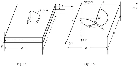
The object of the investigation is a rectangular plate with sides a and b and thickness h, subjected to a dynamic loading p(x,y,t) perpendicular to the plate (Fig. 1 a). The presence of a defect can be modelled as a reduction of the plate thickness or a stiffness reduction and therefore a variation of the flexural rigidity in the governing equations is used. The basic equations of the plate motion are described below.

2.1 Geometrical relationships

The strain and curvature-displacements relationships associated with the mid-plane of the plate for large displacements and shear can be expressed as:

0 _, 0

xz x yz y

w w

x y

ε =ψ +∂ ε =ψ +∂

∂ ∂ ,

0 x_, 0 y _, 0 x y

x y xy

k k k

x y y x

ψ ψ

ψ ∂ ψ ∂

∂ ∂

= = = +

∂ ∂ ∂ ∂ (1 a, f)

and the strain vector is given by:

(2)

where f z( ) is a function describing the distribution of the shear strain along the plate thickness, u(x,y,t) and v(x,y,t) are the in-plane displacements, w x y t

(

, ,

)

is the transverse

displacement and ψ_x

(

x y t, ,

)

, ψ_y

(

x y t, ,

)

are the angles of the rotation of the normal of the cross section to the plate mid-plane (see Fig. 1 b.).

2.2 Constitutive equations

2 2

0 1 0 1 0

, , ,

2 2

x y xy

u w v w u v w w

x x y y y x x y

ε =∂ + _∂ _ ε =∂ + _∂ _ ε = ∂ +∂ +∂ ∂

∂ ∂  ∂ ∂  ∂ ∂ ∂ ∂

{

0 0_, 0 0_, 0 0 _{, ( )} 0_{, ( )} 0

}

T x zkx y zky xy zkxy f z xz f z yz

ε ε ε ε ε

= + + +

Assuming that the material of the plate is linear elastic and isotropic the relations for the generalized stress and strain components are given by:

0 0 0 0 1 0

( ), ( ),

2

x x y y y x xy xy

v N =A ε +νε N = Aε +νε N = − Aε

0 0 0

2 0 2 0

1

( ), ( ), (1 ) ,

2

1 1

(1 ) , (1 )

2 2

o o

x x y y y x xy xy

x xz y yz

M D M D M D

Q k A Q k A

κ νκ κ νκ ν κ

ν ε ν ε

= + = + = −

= − = −

(3 a-h)

(4 a,b) where E is the Young modulus, ν is the Poison ratio, k2 is a shear correction factor which is assumed equal to 5/6 throughout the paper [25]. In Eqns. (3) Nx, Ny and Nxy are

the stress resultants in the mid-plane of the plate, Mx, Myand Mxy are the stress couples

and Qx and Qy are the transverse shear stress resultants.

2.3 Equations of motion

The equilibrium equations may be deduced by considering the translational equilibrium in the x, y and z directions and the rotational equilibrium about x and y which are as follows: 0 0 xy x x y xy y N N hu x y N N hu y x ρ ρ ∂ ∂ + + = ∂ ∂ ∂ ∂ + + = ∂ ∂ 3 2 3 2 0 12 0 12 xy x x x x

y xy y

y y

M

M h

Q c

x y t

M M h

Q c

y x t

ψ ρ ψ ∂ ψ ρ ψ ∂ ∂ ∂ ∂ + − + + = ∂ ∂ ∂ ∂ ∂ + − + + = ∂ ∂ (5 a-c)

2 2 2

1

2 2 2

y x

x y xy

Q

Q w w w w

N N N c hw p

x y x y x y ∂ t ρ

∂ ∂ ∂ ∂ ∂ ∂ + + + + + + = − ∂ ∂ ∂ ∂ ∂ ∂ 2 2 ( , ) ( , ) ( , ) ( , ) ( , ) , ( , ) 1 12

E x y h x y A x y h x y

A x y D x y

v

= =

Here and throughout in the paper dots over variables represents the derivative with respect to the time, c1 and c2 denote the damping coefficients, and ρ is the density of the

plate material.

2.4. Boundary and initial conditions

In the present work fully clamped plates, i.e. plates for which all their four edges are clamped and in-plane fixed, are considered. This means that all displacements u, v and w and angular rotations ψ_x andψ_y are zero along the boundaries.

The initial conditions are accepted in the following general form:

(

₀

)

0

(

₀

)

0

w x y, , =w x y( , ), w x y, , =w x y( , ),

(

₀

)

0

(

₀

)

0

[

₀

]

[

₀

]

x x y x x y y x y y x y x a y b

ψ

, , =

ψ

( , ),

ψ

, , =

ψ

( , , ), ∈ , , ∈ , (6a-d)

3. SOLUTION OF THE PROBLEM

3.1 Reorganizing the equations of the plate motion

Making the widely accepted assumption that mid-plane inertia effects are negligible , i.e.

0

x y

hu hu

ρ =ρ = and moving the nonlinear terms to the right hand side, the equations of motion (5)are written in the following form:

(

1

)

2

u

A

u v u v

A G

x x y y y x

ν ν     ₋   ∂ ∂ ∂ ∂ ∂ ∂ + + + =       ∂  ∂ ∂  ∂  ∂ ∂ 

(

1

)

2

v

A v

v u v u

A G

y y ν x x x y

    ₋  

∂ ∂ ∂ ∂ ∂ ∂

+ + + =

     

2 2

2 2 2 2 3

2

2 2

2 2 2 2 2 2 3

2

2 2

(1 ) (1 )

0

2 2 12

(1 ) (1 )

2 2 12

y y

x x

x x x

y x y x

y y y

D k A w h

D c

x y x y x

x y

D k A w h

D c

x y x y y

y x

ψ ψ

ψ ν ψ ν ρ

ν ν ψ ψ ψ

ψ ψ ν ψ ψ ν ρ

ν ν ψ ψ ψ

_{∂ ∂}  ₋ _{∂ ∂}  _{−  ∂ }  ₊ ₊  ₊ _{−  + + + =}  _{∂ ∂ ∂}   _{∂ ∂ ∂}  _{ ∂ }     _{∂ ∂}  ₋ _{∂ ∂}  _{−  ∂ }  ₊ ₊  ₊ _{−  + + +}  _{∂ ∂ ∂}   _{∂ ∂ ∂}  _{ ∂ }     0 = 2 2 3 1 2 2 (1 ) 2 y x L

v kА w w w

c hw p G

x x y y t

ψ ψ ρ ∂ ∂ _∂  − ∂ ∂ ∂ + + + + + = − +    _{∂ ∂ ∂ ∂}    where 2 2

0.5 0.5 (1 )

u w w w w

G A A

x x y y ν x y

  _{ }  _{  }

∂  _∂  ∂ _ ∂ ∂ ∂ = −    +  −  −  

∂ _ _ ∂  ∂  __ ∂   ∂ ∂  (8 a,b)

2 2

0.5 0.5 (1 )

v w w w w

G A A

y x y x ν x y

  _{ }  _{  }

∂  _∂  ∂ _ ∂ ∂ ∂ = −    +  −  −  

∂ _ _∂  ∂  __ ∂   ∂ ∂ 

and G3_L, denotes the component of the vector G_L(0, 0,G_L3) which is called “nonlinear

force vector due to finite displacements”( see [21, 22].). G3_L has the form:

(

)

2 2 2

3

2 2 2

L x y xy

w w w

G x y t N N N

x y x x  _{∂ ∂ ∂}  = −_ + + _ ∂ ∂ ∂ ∂  

, , (9)

3.2. Numerical approach

Assuming Gu and Gv _{are known functions, Eqns. (7 a-b) form a linear system of PDEs} which can be solved numerically. The solution is obtained using a finite a difference method by applying a central differences formula (see Appendix).

Thus, the generalized displacements vector U=

{

αψ αψ_x, _y,w

}

T (α=h2_{/12) is expanded}

as a sum of the product of the vectors of the pseudo-normal modes Un and the time

dependent functions qn(t) as follows:

U=

1

f

N

n n

n

x y q t =

∑

U ( , ) ( ). (10)

Substituting Eqn. (10) into Eqns. (7 c-e), multiplying by Um(x,y), integrating the product

over the plate surface, invoking the orthogonallity condition, and assuming “proportional damping” in the sense

∫∫

(

c₂ψ_xn2 +c₂ψ2_yn+c w_{1 n}2

)

dxdy=2ξ ω_{n n, the}

equations for _qn(t) will be “uncoupled” in the form:

2

2

n n n n n n n

q t( )+ ξ ω q +ω q t( )=F t( ), (11)

where ω_{n are the natural frequencies of the linear elastic (undamped) Mindlin plate,} ξ_n

are the modal damping parameters and

T

n n L

F t( )=

∫∫

U [P( , , ) G ( , , )]x y t + x y t dxdy , (12a-b)

0 0 T

r t = −p

P( , ) ( , , ) .

The initial conditions defined by Eqns (6) are transformed also in terms of q_n(0) and (0)

n

q :

0 0

(0) , (0) ,

n n n n

q =q q =q (13 a-d)

(

)

(

)

0 0 0 0 0 0 0 0

n n x xn y yn n n x xn y yn

q =

∫∫

w w +αψ ψ +αψ ψ dxdy q, =

∫∫

w w +αψ ψ +αψ ψ dxdy Using the methodology developed by Kukreti and Issa [21] the pseudo-load vector {P+G} is interpolated by a quadratic time dependent polynomial, i.e.

2

( , , )x yτ + ( , , )x yτ = ( , )x y + ( , )x yτ + ( , )x yτ , 0 ≤ ≤τ L_t

Where L_t = t_i+1- t_i represents the time increment, and τ which is defined as τ = -t t_i, identifies a new time origin for each time increment.

Denoting

0 x y = x y 0 1 x y = x y mLt 2 x y = x y Lt

P ( , ) P( , , ), P ( , ) P( , , ), P ( , ) P( , , ),

0 1

2

0

0 1 0 0

t t

x y x y x y x y mL

x y x y L m x a y b

= =

= < < < < < < G ( , ) G( , , ),G ( , ) G( , , ),

G ( , ) G( , , ) , , (15)

the expressions for the constants A, B and C are derived in terms of P_{i and} G_{i (i = 1} to 3). The general solution of Eqn. (14) is given by:

0 0

1 2 1 2 3

( )

n n n n n n n n n n n

q τ =E q +E q +F a +F b +F c (16)

where E1n, E2n, F1n, F2n, F3n denote complicated mathematical expressions

containingω ξ_n, _nandτ (see [22] ) and

T

n n n

a =

∫∫

U A dxdy , b_n=

∫∫

U BT_{n n}dxdy c, _n=

∫∫

U CT_{n n}dxdy (17) The iteration procedure applied to solve the above equations (11) is identical to the ones for circular plates and beams given in [22, 23]. This is why it is summarised very briefly here.

We first solve the eigen-value problem for the plate described by the small deflection Mindlin plate theory which gives the frequencies of free vibration, the normal modes of vibration Un, and the necessary derivatives. Then the initial values qn0 and

0

n

q are computed according to Eqns. (13).

At each time-step [_{ti ,t}i+1] an iteration procedure is applied. It includes solving the small

deflection plate theory equations and then using the obtained values of w and its derivatives to compute Gu and Gv , solve the system of algebraic equations (A1,A2) for

u and v, and then form the nonlinear force vector GL, and solve the system of ODE (11)

and

U Uat the end of the previous time interval are used as initial conditions. The iterative procedure is repeated until the convergence criterion is fulfilled.

The integrals in Eqns. (12, 13 and 17) are evaluated by numerical quadrature following the Simpson rule.

4. Damage identification technique

There are a lot of techniques to treat nonlinear structural response in the time domain. As mentioned above, the state-space representation of the structural vibration response is a suitable and powerful tool for studying the dynamic behaviour of a structure. A standard technique for dealing with phase space

(

w w t, ,

)

of periodically driven oscillators is to

study the projection of

(

w w,

)

at moments in time t, where t is a multiple of the period T=2π/ω. Here ω can be the frequency of the excitation of the mechanical system, an eigen frequency of the structure, or its multiple, and T is a period of the forcing function, an eigen period of the system, or its multiple. The result of inspecting the phase projection

(

w w,

)

only at specific times t=kT is a sequence of dots, representing the so-called Poincaré map. The steady-state converging trajectories, which represent the attractor, are usually formed in the phase space and in many cases of nonlinear systems they are very sensitive to any changes in the system.

The idea of the approach presented here is based on the following considerations:

1. A Poincaré map can be interpreted as a discrete representation of the dynamic system in a state space which is one dimension smaller than the original continuous space of the dynamic system. Since it preserves many properties of periodic and quasiperiodic orbits of the original system and has a lower dimension, it is often used for analyzing the original system. 2. The Poincaré maps contain data for the displacements and the velocities of

purposes becomes obvious. Even when the damage is small, and the responses of the damaged and the healthy structure are close to each other, the points from the Poincaré map are easier to use for comparison and identification purposes because the number of these points is much smaller than the enormous number of points in the time-history diagrams.

According to the above considerations the following damage index can be introduced for the i-th node:

u d

d i i

i u i S S I S − = ,

(

) (

)

1 2 2

, 1 , , 1 ,

1

p

N

u u u u u

i i j i j i j i j

j

S w w w w

−

+ +

=

=

∑

− + − (18 a-c)

(

) (

)

1

2 2

, 1 , , 1 ,

1

p

N

d d d d d

i i j i j i j i j

j

S w w w w

−

+ +

=

=

∑

− + −

where, i=1,2…Nnodes, Nnode is the number of nodes, Np is the number of points in the

Poincaré map and (w w_iju, _iju) and (w_ijd,w_ijd) denotes the j th point on the Poincaré maps of the undamaged and the damaged states, respectively.

A small (close to 0) damage index will indicate no damage, while a big damage index will indicate the presence of a fault at the corresponding location. The above damage index depends on the location of the point on the plate, and consequently it is a function of the plate coordinates x and y. One can expect that the maxima of the surface

( , )

d

d d

I x y (18a) will represent the location of the damage, i.e. _maxd ( _d, _d) max

{ }

_id

i

I x y = I .

for i-th node. Therefore the damage index is defined as the relative difference between these two lengths. The logical expectations are that:

1) Since the fault influences the vibration response of the plate it will introduce changes in the Poincaré map. The differences between the Poincaré maps of the healthy and damaged plates will be indicative of the presence of damage.

2) At the nodes close to the damaged area the introduced damage index I_id (18 a) will be larger than the index for points which are far from the damaged zone. This can be used to localize the detected damage.

5. THE CASE STUDY

This study focuses on damage assessment in rectangular and square plates. The material characteristics of the plates are: Young modulus E = 7.1010 N/m2, Poison ratio ν=0.34,

density ρ= 2778 kg/m3. The damping coefficient _{1 2}

2

12

c c

h

= in Eqns ( 7 ) was chosen to

be 0.00075

3

N s

m . The square plate has dimensions a=b=0.5 m and thickness h= 0.006 m. Two cases of damage were considered: - A) almost central damage- thickness reduction in a small area located in the central part of the plate slightly moved from the centre (one element up and one element left) (see Fig. 2); B) side damage- thickness reduction in a small area close to the left lower corner of the plate as shown in Fig. 2. A finite element model of the plate is shown in Fig. 2.

reduction. In both cases (rectangular and square plates) the thicknesses of the damaged areas are equal to half the thickness of the undamaged plate.

The aim of the following numerical example performed is to test the suggested procedures to detect and localise damage in the plate.

6. SOME RESULTS

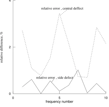
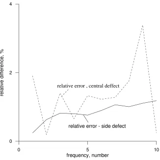
In this paragraph some result for the detection and the localisation of the defects described above in the square and the rectangular plates considered are discussed. First of all the sensitivity of the first ten natural frequencies of the plate was tested. Our results show that in these particular cases both defects introduce very small or nearly no changes in the first 10 natural frequencies of the plate. The relative differences between the frequencies of the intact and the damaged square and rectangular plates are shown in Figs. 4 and 5, respectively. Especially for the case B) the differences between the frequencies are very small and are in the range of the accuracy of its experimental determination. So in these particular cases there is obviously a need for an alternative method.

subjected to a harmonic loading uniformly distributed over the plate surface. Numerical experiments were carried out for different values of the excitation frequency.

In the case of a square plate with a central defect (case A) the excitation frequency was chosen equal to ωe=1000 rad/s. In order to show the applicability of the methods for

higher frequencies for the case B the excitation frequency was ωe=2000 rad/s. (The first

two natural frequencies of healthy plate are ω1=1326.32 rad/s, ω2=2700.3 rad/s ) The

amplitude of the harmonic loading was 6 N.

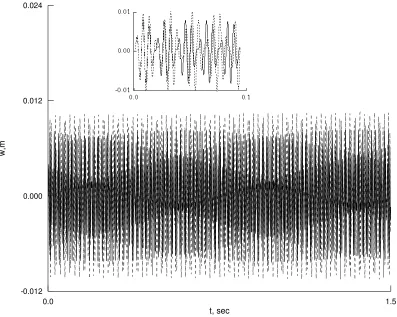
Let us first have a look at the time histories of the plate response for the undamaged and the damaged cases. Figures 6 and 7 give parts of the time histories for the case of central defect and side defect compared to those for the non damaged plate. It can be observed that the applied load leads to large amplitude vibrations of the plate. Due to the fact that the excitation frequency is close to the first natural frequency of the plate a beating phenomenon occurs. It can be appreciated from Figures 6 and 7 that the time histories undergo changes with damage. As expected, the differences for case A central defect are bigger than the differences for case B side defect. It can be seen that close to the origin (t=0) the responses almost coincide with each other (especially for case B) but then the phase shifts and the differences between the responses increase.

slices, called contours, on a 2-dimensional plane. That is, for a given value of z, lines are drawn that connect the (x,y) coordinates that correspond to this particular value of z.

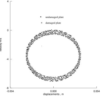
The influence of the damage on the Poincaré maps at the plate centre can be seen in Figures 8 and 9. As can be expected the influence of the central damage (case A) on the Poincaré maps of the plate is larger than the influence of the side defect (case B). The introduced damages do not change the type of the Poincaré section (circle) they only influence the length of the curves formed by the Poincaré dots. Then the damage index

d i

I was calculated for the points from the Poincaré maps for all the nodes and its contour

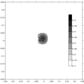
plots were obtained. Fig. 10 details the contour plots of I_id for case A defect for all the plate nodes. As can be seen from this plot case A damage can be detected and localised quite precisely.

Fig. 11 presents analogous contour plots for the case of side damage (case B). It can be observed that the plot identifies quite precisely the position of the defect in spite of the fact that the absolute values of the differences in the displacements and the velocities of the two responses at the nodes of the damaged area are small. The calculations for smaller values of damage (hdamaged/h = 0.66) still show very good prediction of the

damage location (not shown here).

Analogous results were obtained for the case of the rectangular plate.

the difference between the responses increases with the time. In spite of the fact that the Poincaré maps at the plate centre (where the deflections and the velocity are the largest) are very close to each others (Fig. 13) the damage index corresponding to the damaged area has the biggest values, which gives the possibility to locate the damage. In Fig. 14 the contour plot of I_id is compared to the FE model of the plate where the damaged area is coloured in white. It can be seen that the damage location is predicted very precisely. The same conclusion applies in the case of the rectangular plate with central damage (see Figs. 15 and 16). As in the case of the square plate the location of the damage is predicted very precisely and even the small non-symmetry of the damage location with respect to the plate centre can be seen on the contour map of I_id.

7. CONCLUSIONS

A numerical approach for studying the geometrically nonlinear vibrations of rectangular plates with and without damage is developed in the paper. The computed time domain responses are used to analyse the dynamic behaviour of plates in the intact condition and of plates with defects. Based on these analyses a damage index and a method for damage detection and damage location have been proposed. The damage assessment method is based on the phase space representation of the time domain nonlinear response of the plate and uses the analysis of the Poincaré map of the response. The developed damage assessment procedure was applied for the test cases of a square and a rectangular

performance. The potential, the sensitivity and the applicability of the developed method still have to be tested for real measurements and for more structures, defects and loading conditions.

ACKNOWLEDGMENTS

APPENDIX. Finite difference scheme for solution of equations for mid-plane displacements.

Applying the central difference formula the equations (7 a, b) are transformed into the following system of algebraic equation with respect to ui,j , vi,j , i=1,2,…Nx, j=1,2,…Ny,

(Nx and Ny are the numbers of nodes along the axis x and y , correspondingly.

1 1 1 1 1

, , , , ,

2 2 2 2 2

1_, 1, 1_, 1, 2 2 , 2 , 1

2 2

1 1 1 1 1

, , , , ,

2 2 2 2 2

, 1 1, 1

2 1 1 2 2 1 1 2 2 1

2 4 4

i j i j i j i j i j

i j i j i j i j

i j i j

x y y

i j i j i j i j i j

i j i j i

y x y x y

A A A A A

A u A u u u

A A A A A

u v v

ν ν ν ν ν ν ν + − + − + + − + + − − + + + − − + + − + +   − −   + −_ + _ + + ∆ ∆ ∆     −  −  + _ + _ − _{ } + − ∆ ∆ ∆  ∆ ∆      1, 1

1 1 1 1

, , , ,

2 2 2 2

1, 1 1, 1 , ,

1 1

2 2

4 4

j

i j i j i j i j

u

i j i j i j i j

x y x y

A A A A

v v G v

ν ν ν ν + − + − + + − − − − − −     + +       ₊  ₌ ∆ ∆ ∆ ∆             (A1) ,

1 1 1 1 1 1

, , , , ,

2 2 2 2 2 2

1, 1 1, 1 1, 1

1 1 1

2 2 2

4 4 4

i j

i j i j i j i j i j

i j i j i j

x y x y x y

A A A A A A

u u u

ν ν ν

ν ν ν

− + + + + − + + − + − − − − −       + + +         ₋  ₊  ∆ ∆ ∆ ∆ ∆ ∆                  

1 1 1 1 1 1 1

, , , , , , ,

2 2 2 2 2 2 2

1, 1 2 , 1 2 2 ,

1 1 1

2 2 2

4

i j i j i j i j i j i j i j

i j i j i j

x y y y x

A A A A A A A

u v v

ν ν ν

ν + − + + − + − + − + − − −     + + +         − + − + ∆ ∆ ∆ ∆ ∆            

1 1 1

, , ,

2 2 2

, 1 1, 1, ,

2 2 2

1 1

2 2

i j i j i j

v

i j i j i j i j

y x x

A A A

v ν v ν v G

− + −

− + −

− −

+ + + =

∆ ∆ ∆ (A2)

Assuming Gu and Gv are known functions the linear system of algebraic equations is

REFERENCES

[1] P.F. Rizos, N. Apragathos, Identification of crack location and magnitude in a cantilevered beam from the vibration modes. Journal of Sound and Vibration 138 (1990), 381-388.

[2] C. Dong, P. Q. Zhang, W. Q. Feng, T. C. Huang, The sensitivity study of the modal parameters of a cracked beam, Proceeding of the 12th IMAC, Honolulu, HW (1994), pp. 98-105.

[3] H.T. Banks, D.J. Inman, D.J. Leo, Y. Wang, An experimentally validated damage detection theory in smart structures. Journal of Sound and Vibration 191 (1996), 859-880.

[4] J. Chance, G.R. Tomlinson, K. Worden, A simplified approach to the numerical and experimental modelling of the dynamics of a cracked beam, Proceedings of the 12th IMAC, Honolulu, HW (1994), pp. 778 – 786.

[5] Y. Yam, D. S. Bayard, R. E. Scheid, Frequency domain identification for robust large space structures control design, ACC Proceedings, San Francisco, C A (1993), pp. 3021-3023.

[6] P. Verboven, E. Parloo, P. Guillaume, M. Van Overmeire, Autonomous structural health monitoring—part I: modal parameter estimation and tracking. Mechanical Systems and Signal Processing 16 (2002), 637–657.

[7] S.W. Doebling, C.R. Farrar, M.B. Prime, D.W. Shevitz, Damage Identification and Health Monitoring of Structural Systems from Changes in Their Vibration Characteristics: A Literature Review, (Report LA-12767-MS,Los Alamos National Laboratory, NM, USA (1996).

[8] J. Cattarius, D.J. Inman, Time domain analysis for damage detection in smart structures. Mechanical Systems and Signal Processing 11 (1997), 409-423.

[9] M Todd., J M Nichols, L M Pecora and L Virgin, Vibration-based Damage Assessment Utilizing State Space Geometry Changes: local Attractor Variance Ratio, Smart Mater. Struct. 10(2001), 1000-1008.

[10] H. T. Banks, D. J. Inman, D.J Leo, Y. Wang, An experimentally validated damage detection theory in smart structures, Journal of Sound and Vibration. 191 (1996), 859-880.

[11] S.L. Tsyfansky, V.I. Beresnevich, Non-linear vibration method for detection of fatigue cracks in aircraft wings. Journal of Sound and Vibration, 236 (2000), 49-60.

[12] U. Andreaus, P. Casini, F. Vestroni, Non-linear dynamics of a cracked beam under harmonic excitation. International Journal of Nonlinear Mechanics, 42 (2007), 566-575.

[14] I. Trendafilova, E. Manoach, M.P. Cartmell, Ostachowicz W., Zak A., An investigation on damage detection in aircrafts panels using nonlinear time series analysis. Key Engineering Materials, 347 (2007), 213–218.

[15] A.C. Okafor, K. Chandrashekhara, Y.P. Jiang, Location of impact in composite plates using waveform-based acoustic emission and gaussian cross-correlation techniques, in: Proceedings of the SPIE, Vol. 2718 (1996), pp. 291–302.

[16] J.B. Bodeux, J.C. Golinval, Modal identification and damage detection using the data-driven stochastic subspace and ARMAV methods. Mechanical Systems and Signal Processing 17 (2003), 83–89.

[17] C.M. Bishop, Novelty detection and neural network validation, in IEE Proceedings: Vision, Image, and Spectral Processing 141 (1994), 217–222. [18] Z. Hou, M. Noori, R.St. Amand, Wavelet-based approach for structural damage

detection. Journal of Engineering Mechanics 126 (7) (2000), 677–683. [19] J. Grabowska, M. Palacz, M. Krawczuk, W. Ostachowicz, I. Trendafilova, E.

Manoach, M. Cartmell, Wavelet analysis for damage identification in composite structures. Key Engineering Materials, Vol. 347 (2007), 253–258.

[20] A. Nag, D.R. Mahapatra, S. Gopalakrishnan, Identification of delamination in composite beams using spectral estimation and a genetic algorithm. Smart Materials and Structures 11 (2003), 899–908.

[21] A.R. Kukreti, H.I. Issa, Dynamic analysis of nonlinear structures by pseudo-normal mode superposition method. Computers and Structures, 19 (1984), 653-663.

[22] E. Manoach, Dynamic large deflection analysis of elastic-plastic Mindlin circular plates. International Journal of Non-Linear Mechanics, 29,(1994), 723-735. [23] E.Manoach, Dynamic large deflection analysis of elastic-plastic beams and plates.

Proceedings of 7th International Conference Recent Advances on Structural Dynamics, Southampton, July 2000, Vol. 1, pp. 389-400.

[24] P. Ribeiro, E. Manoach, The effect of temperature on the large amplitude vibrations of curved beams. Journal of Sound and Vibration, 285 (2005), 1093-1107.

[image:23.612.105.573.104.355.2]

Fig 1 a Fig. 1 b

Figure 1. a

b

h x

y

p(x,y,t)

O(x,y,z)

z,w

a

b

x,u

y,v

w

ψx

ψy

x

[image:24.612.187.423.56.298.2]

[image:25.612.115.498.61.155.2]

0 5 10

frequency number

0 2 4

re

la

ti

v

e

d

if

fe

re

n

c

e

,

%

relative error , central deffect

[image:26.612.124.492.90.450.2]

relative error , side defect

0 5 10

frequency, number

0 2 4

re

la

ti

v

e

d

if

fe

re

n

c

e

,

%

relative error , central deffect

[image:27.612.144.470.83.410.2]

relative error - side defect

0.0 1.5 t, sec

-0.012 0.000 0.012 0.024

w

,m

[image:28.612.108.505.59.376.2]

0.0 _{time, s} 1.5 -0.005

0.000 0.005 0.010

w

,

[image:29.612.135.476.86.423.2]

m

-0.008 0.000 0.008

displecemnts, m

-5 0 5 10 15

v

e

lo

c

it

y

,

m

/s

[image:30.612.125.483.60.419.2]

undamaged plate damaged plate

-0.004 0.000 0.004 displacements , m

-8 -4 0 4

v

e

lo

c

it

y

m

/s

undamaged plate

[image:31.612.130.486.216.554.2]

damaged plate

-0.25 -0.2 -0.15 -0.1 -0.05 0 0.05 0.1 0.15 0.2 0.25 -0.25

-0.2 -0.15 -0.1 -0.05 0 0.05 0.1 0.15 0.2 0.25

0.11 0.115 0.12 0.125 0.13 0.135 0.14 0.145 0.15

[image:32.612.164.444.134.414.2]

-0.25 -0.2 -0.15 -0.1 -0.05 0 0.05 0.1 0.15 0.2 0.25 -0.25

-0.2 -0.15 -0.1 -0.05 0 0.05 0.1 0.15 0.2 0.25

[image:33.612.163.447.156.444.2]

0.12 0.13 0.14 0.15 0.16 0.17 0.18 0.19 0.2 0.21 0.22 0.23 0.24 0.25

0 10 time, s

-0.15 0.00 0.15

w

,

[image:34.612.160.451.79.343.2]

m

-0.08 0.00 0.08

displacements, m

-30 -20 -10 0 10

v

e

lo

c

it

y

,

m

/s

undamaged plate

[image:35.612.153.462.108.405.2]

damaged plate

[image:36.612.105.585.86.342.2]

Figure 14.

-5 -4 -3 -2 -1 0 1 2 3 4 5

-1 0 1

-0.1 -0.1 0.0 0.1 0.1

displacements, m

-50 -25 0 25

v

e

lo

c

it

y

,

m

/s

undamaged plate

[image:37.612.137.473.58.395.2]

damaged plate

[image:38.612.102.508.109.346.2]

Figure 16.

-5 -4 -3 -2 -1 0 1 2 3 4 5

-1 0 1

FIGURE CAPTIONS

Figure 1. . Plate geometry and coordinate system. a) Plate dimensions and loading, b) Mid-plane of the plate and the components of the generalized displacement vector.

Figure 2. Square plate with central defect and side defect

Figure 3. Rectangular plate with central defect and side defect

Figure 4. Differences between the eigen frequencies of the damaged and undamaged square plate. Solid line – side defect; dashed line - central defect

Figure 5. Differences between the frequencies of the damaged and undamaged rectangular plate in the case of central and side defects

Figure 6. Time histories of the plate centre in the case of central defect solid line – undamaged plate; dashed line – damaged plate. Excitation frequency ωe=1000 rad/s,

p=6 N.

Figure 7 Time histories of the plate centre of the square plate for the case of side defect. Solid line –undamaged plate; Dashed line – damaged plate. Excitation frequency ωe=2000 rad/s, p=6 N.

Figure 8. Poincaré map of the centre of the plate in the case of central damage.

Figure 9. Poincaré map of the centre of the plate in the case of side damage.

Figure 10. Contour map of damage index Id for central damage.

Figure 11. Contour map of damage index Id for square plate with side damage

Figure 12 Time-history diagram for the plate centre of the rectangular plate in the case of side defect. Harmonic loading with P=500 N, ωe=260 rad/s . Solid line – undamaged

Figure 13. Poincaré map for undamaged and damaged in the plate centre of a rectangular plate with a side defect.

Figure 14. Contour map of damage index Idfor rectangular plate with a side defect\

Figure 15 . Poincaré map for undamaged and damaged rectangular plate with a central defect.