A fast algorithm for matrix balancing

PHILIP A. KNIGHT∗ANDDANIEL RUIZ†

Abstract. As long as a square nonnegative matrixAcontains sufficient nonzero elements, then the matrix can be balanced, that is we can find a diagonal scaling ofAthat is doubly stochastic. A number of algorithms have been proposed to achieve the balancing, the most well known of these being Sinkhorn-Knopp. In this paper we derive new algorithms based on inner-outer iteration schemes. We show that Sinkhorn-Knopp belongs to this family, but other members can converge much more quickly. In particular, we show that while stationary iterative methods offer little or no improvement in many cases, a scheme using a preconditioned conjugate gradient method as the inner iteration can give quadratic convergence at low cost.

Key words.Matrix balancing, Sinkhorn-Knopp algorithm, doubly stochastic matrix, conjugate gradi-ent iteration.

AMS subject classifications.15A48, 15A51, 65F10, 65H10.

1. Introduction. For at least 70 years, scientists in a wide variety of disciplines have attempted to transform square nonnegative matrices into doubly stochastic form by applying diagonal scalings. That is, given A ∈ Rn×n_{, A ≥ 0, find}

di-agonal matrices D1and D2so thatP = D1AD2 is doubly stochastic. Motivations

for achieving this balance include interpreting economic data [1], preconditioning sparse matrices [16], understanding traffic circulation [14], assigning seats fairly af-ter elections [3], matching protein samples [4] and ordering nodes in a graph [12]. In all of these applications, one of the main methods considered is SK1. This is an iterative process that attempts to findD1andD2by alternately normalising columns

and rows in a sequence of matrices starting withA. Convergence conditions for this algorithm are well known: ifAhas total support2then the algorithm will converge linearly with asymptotic rate equal to the square of the subdominant singular value ofP[22, 23, 12].

Clearly, in some cases the convergence will be painfully slow. The principal aim of this paper is to derive some new algorithms for the matrix balancing problem with an eye on speed, especially for large systems. First we look at a simple Newton method for symmetric matrices, closely related to a method proposed by Khachiyan and Kalantari [11] for positive definite (but not necessarily nonnegative) matrices. We will show that as long as Newton’s method produces a sequence of positive it-erates, the Jacobians we generate will be positive semi-definite and that this is also true when we adapt the method to cope with nonsymmetric matrices.

To apply Newton’s method exactly we require a linear system solve at each step, and this is usually prohibitively expensive. We therefore look at iterative techniques for approximating the solution at each step. First we look at splitting methods and we see that SK is a member of this family of methods, as is the algorithm proposed by Livne and Golub in [16]. We give an asymptotic bound on the (linear) rate of conver-gence of these methods. For symmetric matrices we can get significant improvement

∗_{Department of Mathematics, University of Strathclyde, 26 Richmond Street, Glasgow G1 1XH}

Scot-land (pk@maths.strath.ac.uk). This work was supported in part by a grant from the Carnegie Trust for the Universities of Scotland.

†_{INPT-ENSEEIHT 2, rue Charles Camichel, Toulouse, France (Daniel.Ruiz@enseeiht.fr)}

1_{The algorithm has been given many different names, Sinkhorn-Knopp is the name usually adopted} by the linear algebra community. We’ll refer to it as SK in the rest of this paper

2_{total support is defined in§3.}

over SK. Unfortunately, we show this is not true for nonsymmetric matrices.

Next we look at a preconditioned conjugate gradient method for solving the inner iteration. We discuss implementation details and show that asymptotically, super-linear convergence is achievable, even for nonsymmetric matrices. By imple-menting a box constraint we ensure that our iterates retain positivity and we demon-strate the reliability and speed of our method in tests. The algorithm, the core of which takes up less than forty lines of MATLAB code, is given in an appendix.

To measure the rate of convergence for an iterative processI we use the root-convergence factor [18,§9.2.1]

R(x) =sup (

lim sup

k→∞

kxk−xk1/k|{xk} ∈C

) ,

whereCis the set of all sequences generated byI which converge tox.

A number of authors have presented alternative techniques for balancing ma-trices that can converge faster than SK. For example, Parlett and Landis [19] look at some simple ways of trying to accelerate the convergence by focusing on reduc-ing statistics such as the standard deviation between row sums of the iterates. In certain cases, they show great improvement is possible, suggesting that the rate on convergence is not dependent on the singular values ofP; but they also give exam-ples where their alternatives perform significantly worse. We include a comparison of one of these algorithms against our proposed approach in§6. Linial et al. [15] use a similar approach to [19] in the context of estimating matrix permanents, although their upper bound on iteration counts (O(n7)) makes them distinctly unappealing for large problems!

A completely different approach is to view matrix balancing as an optimisation problem. There are many alternative formulations, perhaps the first being that of Marshall and Olkhin [17] who show that balancing is equivalent to minimizing the bilinear formxTAysubject to the constraintsΠxi = Πyi = 1. However, the

exper-imental results we have seen for optimisation techniques for balancing [17, 21, 2] suggest that these methods are not particularly cheap to implement.

2. Newton’s method. Let D : Rn → Rn×n _{represent the operator that turns a}

vector into a diagonal matrix,D(x) =diag(x), and leterepresent a vector of ones. Then to balance a nonnegative matrix, A, we need to find positive vectors randc such that

D(r)AD(c)e=D(r)Ac=e, D(c)ATr=e. (2.1)

Rearranging these identities gives

c=D(ATr)−1e, r=D(Ac)−1e,

and one way of writing SK [9, 12] is as

ck+1=D(ATrk)−1e, rk+1=D(Ack+1)−1e.

(2.2)

IfAis symmetric then (2.1) can be simplified. To achieve balance we need a vector x∗that satisfies

f(x∗) =D(x∗)Ax∗−e=0.

This leads to the iterative step

xk+1=D(Axk)−1e.

(2.4)

Exactly the same calculations are performed as for (2.2), one simply extractsrkand

ckfrom alternate iterates [12]. IfAis nonsymmetric, one can use (2.4) on

S=

0 A AT 0

.

An obvious alternative to SK is to solve (2.3) with Newton’s method. Differenti-ating f(x)gives

J(x) = ∂

∂x(D(x)Ax−e) =D(x)A+D(Ax),

a result that is easily confirmed by componentwise calculation or with tensor algebra, hence Newton’s method can be written

xk+1=xk−(D(xk)A+D(Axk))−1(D(xk)Axk−e).

We can rearrange this equation to get

(D(xk)A+D(Axk))xk+1=D(Axk)xk+e,

so,

(A+D(xk)−1D(Axk))xk+1=D(xk)−1(D(Axk)xk+e)

= Axk+D(xk)−1e,

(2.5)

and we can set up each Newton iteration by performing some simple vector opera-tions and updating the diagonal on the left hand side. This matrix plays a key role in our analysis and we introduce the notation

A_k= A+D(xk)−1D(Axk).

Note that the matrix on the lefthand side of (2.5) inherits the symmetry ofA. This algorithm can be implemented by applying one’s linear solver of choice. In practical applications, it makes sense to apply an inner-outer iteration scheme. In§4 and§5 we look at some efficient ways of doing this. In particular, we look at how to deal with the nonsymmetric case. Here, we can use the same trick we used to derive (2.4) but, as we’ll see, the resulting linear systems are singular.

The idea of using Newton’s method to solve the scaling problem is not new and was first proposed by Khachiyan and Kalantari in [11]. Instead of (2.3), the equivalent equation

Ax− D(x)−1e=0 (2.6)

work for their formulation. In§5 we explain why our approach leads to faster con-vergence.

Newton’s method is also used as a method for solving the balancing problem for symmetric matrices in [16]. Here the authors work with

I− ee

T

n

D(Ax)x=0 (2.7)

instead of (2.3). They then use a Gauss-Seidel Newton method to solve the problem and show that this approach can give significant improvements over SK. We will develop this idea in§4.

Yet another formulation of (2.4) can be found in [7], where the author suggests the resulting equation is solved by Newton’s method. However no attempt is made to implement the suggested algorithm and the fact that only the righthand side changes in the linear system that is solved at each step suggests that rapid conver-gence is unlikely in general.

3. Properties ofA_k. In order that we can solve the balancing problem efficiently, in particular whenAis large and sparse, we will use iterative methods to approxi-mately solve the linear system in (2.5). There are a number of possibilities to choose asAk, the matrix on the lefthand side of the expression, is symmetric positive

semi-definite. This is a consequence of the following result (which doesn’t require sym-metry).

THEOREM 3.1. Suppose that A∈ Rn×n _{is nonnegative and y∈ R}n _{is positive. Let}

D=D(Ay)D(y)−1. Then for allλ∈σ(A+D),Re(λ)≥0.

Proof. Note thatA+Dis similar to

D(y)−1(A+D)D(y) =D(y)−1AD(y) +D(y)−1D(Ay)

=D(y)−1AD(y) +D(D(y)−1AD(y)e)

=B+D(Be),

where B = D(y)−1AD(y). Now Be is simply the vector of row sums ofB and so adding this to the diagonal ofBgives us a diagonally dominant matrix. Since the diagonal is nonnegative, the result follows from Gershgorin’s theorem.

IfAhas a nonzero entry on its diagonal then at least one of the rows ofB+D(Be) will be strongly diagonally dominant and, by a theorem of Taussky [24], it will be nonsingular. We can also ensure thatAkis nonsingular by imposing conditions on

the connectivity between the nonzeros inA. We can establish the following result. THEOREM3.2. Suppose that A ∈ Rn×n is nonnegative. If A is fully indecomposable

thenA_kis nonsingular.

Recall that a matrixAis fully indecomposable if it is impossible to find permu-tation matricesPandQsuch that

PAQ=

A1 0

A2 A3

withA1andA2square (a generalisation of irreducibility).

The proof of Theorem 3.2 is postponed to the end of the section. However in many cases we will not be able to satisfy its conditions. For example, ifAis nonsym-metric and we use Newton’s method to balance

S=

0 A AT 0

thenSis not fully indecomposable. In fact it is straightforward to show that in this case the linear systems we have to solve are singular.

We’d also like to use our new algorithms on any nonnegative matrix for which balancing is possible, namely any matrix which has total support (A ≥ 0 has total support ifA6=0 and all the nonzero elements lie on a positive diagonal). Matrices that have total support but that aren’t fully indecomposable also lead to singular systems in (2.5).

Singularity in these cases is not problematic as the systems are consistent. As Theorem 3.5 shows, we can go further, and we can solve the systems whenever A has support (A≥0 has support if it has a positive diagonal).

We need some preliminary results.

LEMMA3.3.Suppose that A∈Rn×n_{is a symmetric nonnegative matrix with support.}

Then there is a permutation P such that PAPT is a block diagonal matrix in which all the diagonal blocks are irreducible.

Proof. We show this by induction on n. Clearly it is true if n = 1. Suppose n > 1 and our hypothesis is true for all matrices of dimension smaller thann. IfA is irreducible there is nothing to prove, otherwise we can find a permutationQsuch that

QAQT=

A1 C

0 A2

=

A1 0

0 A2

,

whereC = 0 by symmetry. Since Ahas support so doesQAQT and henceA1and

A2must each have support, too and we can apply our inductive hypothesis.

LEMMA3.4. Suppose that A≥0has support and let B= A+D(Ae). If either A is symmetric or it is irreducible then the null space of B is orthogonal to e and the null space has a basis whose elements can be permuted into the form



 e

−e 0



.

(In the case that the null space has dimension one, the zero component can be omitted). Proof. IfBis nonsingular we have nothing to prove, so we assume it is singular (and hence by Taussky’s theorem [24],Ahas an empty main diagonal).

From Theorem 2.3 and Remark 2.9 in [13] we can infer that if B is irreducible then the null space is one dimensional and, since it is weakly diagonally dominant, all components are of equal modulus. All that remains is to show that there are an equal number of positive and negative components in elements from the null space and hence they can be permuted into the required form.

We choose a permutationi1,i2, . . . ,inof 1, . . . ,nsuch that for 1≤j≤n,bijij+1 6=

0, wherein+1 = i1. Such a permutation exists because Ahas support and has an

empty main diagonal. Now suppose that x is in the null space of B. Since B is diagonally dominant, the sign ofximust be opposite to that ofxjwheneverbij 6=0

(i6=j). By construction,xij =−xij+1for 1 ≤j≤n. This is only possible ifnis even,

in which casexTe=0, as required.

IfB is not irreducible but is symmetric then (by the previous lemma)PBPT = diag(B1,B2, . . . ,Bk)where theBiare irreducible. Since the null space ofBis formed

THEOREM 3.5. Suppose that A ∈ Rn×n _{is a symmetric nonnegative matrix with}

support and that y>0. The system

(A+D(Ay)D(y)−1)z= Ay+D(y)−1e

is consistent.

Proof. Let Ay = D(y)AD(y). Since (Ay+D(Aye)) is symmetric, elements

or-thogonal to its null space must lie in its range, so as a consequence of the previous lemma, we can find a vectordsuch that

(Ay+D(Aye))d=e.

Letz=y/2+D(y)d. Then

(A+D(y)−1D(Ay))z= 1

2(A+D(Ay)D(y)

−1

)y

+D(y)−1(D(y)AD(y)d+D(Ay)D(y)d)

= Ay+D(y)−1(Ay+D(Aye))d

= Ay+D(y)−1e.

While we have proved that Newton’s step will converge ifxk >0, we have not

shown thatxk+1 >0. In fact, it needn’t be, and this will be an important

considera-tion for us in developing balancing methods in the later secconsidera-tions. To finish the section, we prove Theorem 3.2.

Proof. LetB= D(xk)−1AD(xk)and considerB+D(Be). Suppose that this

ma-trix is singular andvlies in its null space. We can apply Lemma 3.4, and we know that exactly half of its components are positive and half are negative. Suppose thatP permutesvso that the first half of the entries ofPvare positive. Then

P(B+D(Be))PT=

D1 B1

B2 D2

,

whereD1andD2are diagonal: otherwise, diagonal dominance would force some of

the entries of(B+D(Be))vto be nonzero. Hence

PBPT=

0 B1

B2 0

.

But such a matrix is not fully indecomposable, contradicting our hypothesis.

4. Stationary iterative methods. If we only want to solve (2.5) approximately, the simplest class of methods to consider is that of stationary iterative methods, in particular splitting methods. AsA_k is symmetric positive semi-definite we know that many of the common splitting methods will converge.

the second largest eigenvalue ofL−1U, whereLis the lower triangular part andU the strictly upper-triangular part ofP+I−2eeT/n. Note that the bound is not in terms ofρ(L−1U)as the matrix in the lefthand side of (2.7) is singular.

In our main result in this section we show that the rate of convergenceR(x∗)

can be ascertained for a much wider class of splitting methods. We use (2.5) rather than (2.7) as it leads to particularly simple representations of the methods.

Suppose thatA_k = Mk−Nk whereMk is nonsingular. We can then attempt to

solve the balancing problem with an inner-outer iteration where the outer iteration is given by the Newton step and the inner iteration by the splitting method

Mkyj+1=Nkyj+Axk+D(xk)−1e,

wherey0 = xk. However, we can update Mkextremely cheaply at any point—we

only need to update its diagonal and the vectors we need for this are available to us at each step—so it seems sensible to run only one step of the inner iteration. In this case, our splitting method for (2.5) becomes

Mxk+1=Nkxk+Axk+D(xk)−1e

= (Mk− D(xk)−1D(Axk))xk+D(xk)−1e

=Mkxk− D(Axk)e+D(xk)−1e

=Mkxk−Axk+D(xk)−1e.

In other words, our iteration can be written

xk+1=xk+M−1k (D(xk)−1e−Axk).

(4.1)

Note that if we chooseMk =D(xk)−1D(Axk)in (4.1), then the resulting iteration

is

xk+1=xk+D(xk)D(Axk)−1(D(xk)−1e−Axk)

=xk+D(Axk)−1e− D(xk)e

=D(Axk)−1e,

and we recover (2.4) hence SK can be neatly classified amongst our splitting methods. To prove a general result we use Theorem 10.3.1 from [18] which in our notation can be stated as follows.

THEOREM4.1. Let f :Rn →Rn_{be Gateaux differentiable in an open neighbourhood}

S0of a point x∗at which f0is continuous and f(x∗) =0.

Suppose that f0(x) = M(x)−N(x)where M(x∗)is continuous and nonsingular at

x∗ and thatρ(G(x∗)) < 1where G(x) = M(x)−1N(x). Then for m ≥ 1the iterative

processI defined by

xk+1=xk− m

∑

G(xk)j−1

!

M(xk)−1f(xk), k=0, 1, . . . ,

(4.2)

has attraction point x∗and R(x∗) =ρ(G(x∗)m).

COROLLARY 4.2. Suppose that A ∈ Rn×n _{is a symmetric nonnegative matrix with}

support. Let x∗ > 0be a vector such that P = D(x∗)AD(x∗)is stochastic. Then for the

iterative process defined by (4.1) R(x∗) = ρ(M−1N)where M−N is the splitting applied

Proof. The existence ofx∗is guaranteed [22]. Letm=1, f(x) =D(x)Ax−eand

letM(xk) =D(xk)Mk. Then (4.1) can be rewritten as (4.2) and

G(xk) =M(xk)−1N(xk) =M−1k Nk.

So in the limit for a sequence{xk}converging tox∗,R(x)is governed by the spectral

radius of the splitting of

lim

k→∞Ak=A+D(x∗)

−1_D(Ax

∗) =A+D(x∗)−2.

For many familiar splittings,R(x∗)has an alternative representation as we can

often show thatρ(M−1N)is invariant under the action of diagonal scaling on A. If

this is the case we can replaceA+D(x∗)−2with

D(x∗)(A+D(x∗)−2)D(x∗) =P+I,

that is the asymptotic rate of convergence can be measured by looking at the spec-tral radius of the splitting matrix forP+I. Many familiar splitting methods exhibit this scaling invariance. For example, the Jacobi method, Gauss-Seidel and succes-sive over relaxation are covered by the following result, whereX◦Yrepresents the Hadamard product of two matrices.3

THEOREM4.3. Suppose that A,H ∈ Rn×n _{and D is a nonsingular diagonal matrix.}

Let M=A◦H and N=M−A. Then the spectrum of M−1N is unchanged if we replace A with DAD.

Proof. Notice thatN=A◦GwhereG=eeT−Hand so

(DAD◦H)−1(DAD◦G) = (D(A◦H)D)−1D(A◦G)D=D−1(A◦H)−1(A◦G)D.

In particular, in the case of Gauss-Seidel, we get a bound comparable with the formulation adopted in [16] mentioned at the start of this section.R(x∗)is usually a

little smaller for Livne and Golub’s method but for sparse matrices the difference is frequently negligible.

For SK, though, we get R(x∗) = ρ(P) = 1. This is because the formulation

described in (2.4) oscillates rather than converges. This phenomenon is discussed in [12], where it is shown that R(x∗)is equal to the modulus of the subdominant

eigenvalue ofP.

IfAis symmetric, then it is possible to significantly improve convergence speed over SK with an appropriate choice ofM. However, things are different ifAis non-symmetric. For example, consider the effect of using Gauss-Seidel in (4.1) where A is replaced by

S=

0 A AT 0

andxk =

r_kT cT_k T. We have,

rk+1

ck+1

=

rk

ck

+

D(Ack)D(rk)−1 0

AT D(ATrk)D(ck)−1

−1

D(rk)−1e−Ack D(ck)−1e−ATrk

.

After some straightforward manipulation, this becomes

rk+1

ck+1

=

D(Ack)−1e

D(ATrk)−1e+ck− D(ck)D(ATrk)−1ATrk+1

. (4.3)

In the spirit of Gauss-Seidel, we can replacerkin the righthand side of (4.3) withrk+1,

giving

rk+1

ck+1

=

D(Ack)−1e D(ATrk+1)−1e

,

and this is precisely (2.2), SK. In other words the Gauss-Seidel Newton method offers no improvement over SK for nonsymmetric matrices.

There are any number of choices forMin (4.1), but in tests we have not been able to gain a consistent and significant improvement over SK whenAis nonsymmetric. As most of the applications for balancing involve nonsymmetric matrices we need a different approach.

5. Conjugate gradient method. Recall that ifAis symmetric and nonnegative the Newton step (2.5) can be written

Akxk+1=Axk+D(xk)−1e,

where A_k = A+D(xk)−1D(Axk). By Theorems 3.1 and 3.5, we know thatAk is

positive semi-definite and (2.5) is consistent wheneverxk >0 and we can solve the

Newton step with the conjugate gradient method [8]. Essentially, all we need to do is to find an approximate solution to (2.5) and iterate, ensuring that we never let components of our iterates become negative. We now look in more detail at how we implement the method efficiently.

First, motivated by the proof of Theorem 3.1, we note that we can apply a diago-nal scaling to (2.5) to give a symmetric diagodiago-nally dominant system. Premultiplying each side of the equation byD(xk)and writingyk+1=D(xk)−1xk+1we get

(Bk+D(Bke))yk+1= (Bk+I)e,

(5.1)

whereBk=D(xk)AD(xk). We needn’t formBkexplicitly, as all our calculations can

be performed withA. The natural choice as initial iterate for every inner iteration4is e, for which the initial residual is

r= (Bk+I)e−(Bk+D(Bke))e=e−Bke=e−vk,

wherevk = xk◦Axk. Inside the conjugate gradient iteration we need to perform a

matrix-vector product involvingBk+D(Bke). For a given vectorp, we can perform

this efficiently using the identity

(Bk+D(Bke))p=xk◦(A(xk◦p)) +vk◦p.

Since the rest of the conjugate gradient algorithm can be implemented in a standard way, this matrix-vector product is the dominant factor in the cost of the algorithm as a whole.

As a stopping criterion for the scaling algorithm we use the residual measure

ke− D(xk)Axkk2=ke−vkk2.

In contrast to our experience with stationary iterative methods, it pays to run the in-ner iteration for a number of steps, and so we need a stopping criterion for the inin-ner iteration, too. As is standard with inexact Newton methods, we don’t need a precise solution while we are a long way from the solution and we adopt the approach out-lined in [10, Chap. 3], using the parametersηmaxto limit the size of the forcing termη

andγto scale the forcing term to the residual measure. In our algorithm the default

values areηmax=0.1,γ=0.9.

While we know thatBk+D(Bke)is SPD ifxk>0, we cannot guarantee that (5.1)

will have a positive solution. Furthermore, we do not know that our Newton method will converge if our initial guess is a long way from the solution. We therefore ap-ply a box constraint inside the inner iteration. We introduce a parameterδ which

determines how much closer to the edge of the positive cone we are willing to let our current iterate move and a second parameter∆bounding how far we can move away. We don’t want components of our scaling to grow too large as this generally forces another component to shrink towards 0. By rewriting (2.5) in the form (5.1) we ensure that all coordinate directions are treated equally. Before we move along a search direction in the conjugate gradient algorithm, we check whether this would move our iterate outside our box. If it does, we can either reject the step or only move part of the way along it and then restart the inner iteration. In our experience, it pays not to reject the step completely and instead we move along it until the minimum element ofyk+1equalsδor the maximum equals∆. In general the choicesδ = 0.1

and∆=3 seem to work well.

We report the results of our tests of the method in the next section. As is to be ex-pected, the fact that the method converges independently of the spectrum of our tar-get matrix means that the conjugate-gradient method has the potential to converge much more quickly than the other methods we have discussed. Our experience is that it is no only quick but it is robust, too.

While stationary iterative methods couldn’t improve on SK for nonsymmetric systems the picture changes for the conjugate gradient method. IfAis nonsymmetric we can apply the symmetric algorithm to

S=

0 A AT 0

.

The resulting method is no longer connected to SK. From the results in§3 we know that the Jacobian will be singular at each step, but that the linear systems we solve will be consistent. AlthoughBkis singular the fact that it is semidefinite and the

sys-tem is consistent means CG will work prvided the initial residual is in the othogonal complement of the kernel of S. We ensure this is the case by settingy0=e. Our tests

show our method is robust in these cases, although the residual may not decrease monotonically, suggesting that the algorithm may be moving between local minima of the functionkD(x)Sx−ek2_.

in solving the large scale balancing problems discussed in [12], where a rank one correction is applied implicitly toA.

As we mentioned early, Khachiyan and Kalantari did not discuss the practical application of their algorithm in [11]. However it too can be implemented using the conjugate gradient method. For this formulation, (5.1) is replaced with

(Bk+I)yk+1=2e.

While this is also straightforward to implement, we can no longer guarantee that the systems will be semi-definite unlessAis, too. In experiments, we have found that the Khachiyan-Kalantari approach is significantly slower than the one we propose.

6. Results. We now compared the performance of the conjugate gradient based approach against a number of other algorithms. The algorithms considered are as follows. BNEWT is our implementation of an inexact Newton iteration with con-jugate gradients; SK is the Sinkhorn-Knopp algorithm and EQ is the ”equalize” algorithm from [19]; GS is a Gauss-Seidel implementation of (4.1). We use this in preference to the method outlined in [16], as for large matrices it is much easier to implement in MATLAB. In terms of rate of convergence, the algorithms are similar.

We have tested the algorithm against both symmetric and nonsymmetric matri-ces. All our tests were carried out in MATLAB. We measure the cost in terms of the number of matrix-vector products taken to achieve the desired level of convergence. In our tests on nonsymmetric matrices, we have counted the number of products in-volvingAorAT_{(double the number for the symmetrised matrixS). We ran our}

algo-rithms until an appropriate residual norm fell below a tolerance of 10−6. For BNEWT, and other algorithms for symmetric matrices, we measuredkD(xk)Axk−ek2

(replac-ingAwithSifAwas nonsymmetric). For SK we measuredkD(ck)ATrk−ek2, where

ckandrkare defined in (2.2). In all cases, our initial iterate is a vector of ones.

In BNEWT there are a number of parameters (ηmax,γ,δand∆) we can tune to

improve performance connected to the convergence criterion of the inner step and the line search. Unless otherwise stated, we have used the default values for these parameters.

Our first batch of test matrices were used by Parlett and Landis [19] to compare their balancing algorithms to SK. These are all 10×10 upper Hessenberg matrices defined as follows. H= (hij)where

hij=

0, j<i−1 1, otherwise,

H2differs fromHin only thath12is replaced by 100 andH3= H+99I. Our results

are given in Table 6.1. In this experiment, the tolerance changed to 10−5as this was the choice in [19]. The algorithm of Parlett and Landis, EQ, uses mainly vector-vector operations, and we have converted this to an (approximately) equivalent number of matrix-vector products.

We see the consistent performance of BNEWT, outperforming the other choices. The results for GS confirm our analysis in§4, showing it is virtually identical to SK. The more fine-grained nature of EQ means that a comparison with other algorithms in terms of operation counts is misleading. In our tests it took a similar number of iterations as SK to converge, and significantly longer time.

We next tested BNEWT on then×n version ofH3. For large values ofn, this

BNEWT SK EQ GS

H 76 110 141 114

H2 90 144 131 150

H3 94 2008 237 2012 TABLE6.1

Rate of convergence for Parlett and Landis test matrices.

elements of the balancing factors grows extremely large (the matrix becomes very close in a relative sense to a matrix without total support). The cost of convergence is given in Table 6.2, along with the ratiorn= (maxixi)/(minixi).

n=10 25 50 100

BNEWT 124 300 660 1792 SK 3070 16258 61458 235478 rn 217 7×106 2×1014 2×1029

TABLE6.2 Rate of convergence for Hn.

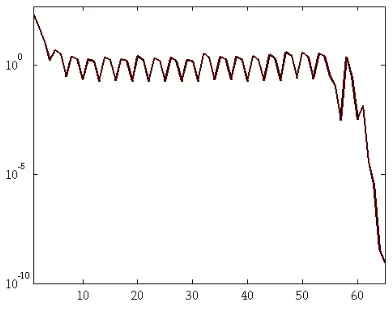
BNEWT still copes in extremely trying circumstances, although the convergence of the residual is far from monotonic (we illustrate the progress after each inexact Newton step forn=50 in Figure 6.1).

FIG. 6.1.Convergence graph of BNEWT for H50.

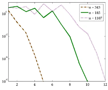
The oscillatory behaviour is undesirable, and it can be ameliorated somewhat by varying the parameters in BNEWT. This is illustrated in Figure 6.2. In terms of cost, the choiceηmax =10−2,δ=0.25 proved best in reducing the matrix-vector product

count to 568.

FIG. 6.2.Smoothing convergence of BNEWT for H50.

the method proves robust and we avoid the oscillatory behaviour we saw for our previous more extreme example.

FIG. 6.3.Convergence of BNEWT for sparse nonsymmetric matrices.

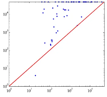
We have also carried out more comprehensive tests on a selection of matrices from the University of Florida Sparse Matrix Collection (UFL)5. First we attempted to scale 45 sparse symmetric matrices with dimensions between 5,000 and 50,000 from the matrix sets Schenk_IBMNAand GHS_indefwhich have been observed to be resistant to scaling algorithms [20]. Each of the algorithms BNEWT, GS and SK was run until our default tolerance was reached or 2,000 matrix-vector products had been computed. In all but one case, BNEWT converged within the limit while GS met the convergence criterion in 25 cases, and SK in only 3. In Figure 6.4 we plot the number of matrix-vector products required by BNEWT (along thex-axis) against the number required by GS. Cases where the algorithms failed to converge in time

lie at the limits of the axes. The three cases where SK converged are circled (in each case requiring significantly more work than the other algorithms). A pattern emerges where GS converges very quickly on “easy” examples but BNEWT is far more robust and almost always converges at reasonable speed.

FIG. 6.4.Comparison of algorithms on sparse symmetric matrices.

Similar tests were carried out on 60 representative nonsymmetric matrices from the UFL collection with dimensions between 50 and 50,000 to compare BNEWT and SK. The results are shown in Figure 6.5. In this case, the algorithms were given up to 50,000 matrix-vector products to converge. We see the clear superiority of BNEWT in these examples, regularly at least 10 times as fast as SK, although on occasions con-vergence wasn’t particularly rapid, particularly when (maxixi)/(minixi) is large.

SK failed to converge in over half the cases.

FIG. 6.5.Comparison of algorithms on sparse nonsymmetric matrices.

these cases, balancing is impossible but an approximate solution can be found. In many cases BNEWT is robust enough to find an approximate solution in reasonable time (nonzero elements which don’t lie on a positive diagonal are almost obliterated by the scaling). Such approximate scalings can be used as preconditioners, but we have found that equally good preconditioners can be found by applying a handful of iterations of SK, even though the resulting diagonal factors do not come close to balancing the matrix.

7. Conclusions. In many applications, the Sinkhorn-Knopp algorithm offers a simple and reliable approach to balancing; but its limitations become clear when the matrices involved exhibit a degree of sparsity (in particular, the a priori measure of convergence given in [6] fails if the matrix to be balanced has even a single zero). We have clearly shown that an inexact Newton method offers a simple way of overcom-ing these limitations. By takovercom-ing care to remain in the positive cone, we see improve-ments for symmetric and nonsymmetric matrices. Further speed ups many be possi-ble by using more sophisticated preconditioning techniques for the conjugate gradi-ent algorithm. In examples where our new algorithm converge slowly the diagonal factors typically contain widely varying components ((maxixi)/(minixi) 1010,

say) and we are not aware of applications for accurate balancing in these cases.

REFERENCES

[1] MICHAELBACHARACH,Biproportional Matrices & Input-Output Change, CUP, 1970.

[2] HAMSABALAKRISHNAN, INSEOKHWANG ANDCLAIREJ. TOMLIN,Polynomial approximation algo-rithms for belief matrix maintenance in identity management, Appears inProceedings of the 43rd IEEE Conference on Decision and Control, Vol. 5 (2004), pp. 4874–4879.

[3] MICHELBALINSKI,Fair majority voting (or how to eliminate gerrymandering), American Mathematical Monthly, 115 (2008), pp. 97–113.

[4] M. DASZYKOWSKI, E. MOSLETHFÆGESTAD, H. GROVE, H. MARTENS ANDB. WALCZAK, Match-ing 2D gel electrophoresis images with Matlab Image ProcessMatch-ing Toolbox, Chemometrics and Intelli-gent Laboratory Systems, 96 (2009), pp. 188–195.

[5] IAINS. DUFF, R. G. GRIMES ANDJ. G. LEWIS,Users’ Guide for the Harwell-Boeing Sparse Matrix Collection (Release I), Technical Report RAL 92-086, Rutherford Appleton Laboratory (1992). [6] JOEL FRANKLIN ANDJENSLORENZ, On the scaling of multidimensional matrices, Linear Algebra

Appl., 114/115 (1989), pp. 717–735.

[7] MARTINF ¨URER,Quadratic convergence for scaling of matrices, in Proc. ALENEX/ANALC 2004, Lars Arge, Giuseppe F. Italiano, and Robert Sedgewick, editors, pp. 216-223, 2004.

[8] MAGNUSR. HESTENES, EDUARDSTIEFEL,Methods of conjugate gradients for solving linear systems, Journal of Research of the National Bureau of Standards, 49 (1952), pp. 409–436.

[9] BAHMANKALANTARI ANDLEONIDKHACHIYAN,On the complexity of nonnegative-matrix scaling, Linear Algebra Appl., 240 (1996), pp. 87–103.

[10] C. T. KELLEY,Solving Nonlinear Equations with Newton’s Method, SIAM, Philadelphia, 2003. [11] LEONIDKHACHIYAN ANDBAHMANKALANTARI,Diagonal matrix scaling and linear programming,

SIAM J. Opt., 2 (1992), pp. 668–672.

[12] PHILIP A. KNIGHT,The Sinkhorn-Knopp algorithm: convergence and applications, SIMAX, 30 (2008), pp.261–275.

[13] L. YU. KOLOTILINA,Nonsingularity/singularity criteria for nonstrictly block diagonally dominant matri-ces, Linear Algebra Appl., 359 (2003), pp. 133–159.

[14] B. LAMOND ANDN. F. STEWART,Bregman’s balancing method, Transportation Research 15B (1981), pp. 239–248.

[15] NATHANLINIAL, ALEXSAMORODNITSKY ANDAVIWIGDERSON,Deterministic Strongly Polynomial Algorithm for Matrix Scaling and Approximate Permanents, Combinatorica, 20 (2000) pp. 545–568. [16] ORENE. LIVNE ANDGENEH. GOLUB,Scaling by binormalization, Numerical Algorithms, 35 (2004),

pp. 97–120.

[18] J. M. ORTEGA ANDW. C. RHEINBOLDT,Iterative Solution of Nonlinear Equations in Several Variables, Academic Press, New York, 1970.

[19] B. N. PARLETT ANDT. L. LANDISMethods for scaling to doubly stochastic form, Linear Algebra Appl., 48 (1982), pp. 53–79.

[20] DANIELRUIZ ANDBORAUCARA symmetry preserving algorithm for matrix scaling, Technical report, INRIA RR-7552 (2011).

[21] MICHEALH. SCHNEIDERMatrix scaling, entropy minimization, and conjugate duality (II): The dual problem, Math. Prog. 48 (1990), pp. 103–124.

[22] RICHARDSINKHORN ANDPAULKNOPPConcerning nonnegative matrices and doubly stochastic matri-ces, Pacific J. Math. 21 (1967) , pp. 343–348.

[23] GEORGEW. SOULES,The rate of convergence of Sinkhorn balancing, Linear Algebra Appl., 150 (1991), pp. 3–40.

[24] OLGATAUSSKY,Bounds for characteristic roots of matrices, Duke Math. J., 15(1948), pp. 1043–1044.

Appendix. The Symmetric Algorithm.

function [x,res] = bnewt(A,tol,x0,delta,Delta,fl) % BNEWT A balancing algorithm for symmetric matrices %

% X = BNEWT(A) attempts to find a vector X such that % diag(X)*A*diag(X) is close to doubly stochastic. A must % be symmetric and nonnegative.

%

% X0: initial guess. TOL: error tolerance.

% delta/Delta: how close/far balancing vectors can get % to/from the edge of the positive cone.

% We use a relative measure on the size of elements. % FL: intermediate convergence statistics on/off.

% RES: residual error, measured by norm(diag(x)*A*x - e). % Initialise

n = size(A,1); e = ones(n,1); res=[]; if nargin < 6, fl = 0; end

if nargin < 5, Delta = 3; end if nargin < 4, delta = 0.1; end if nargin < 3, x0 = e; end if nargin < 2, tol = 1e-6; end

g=0.9; etamax = 0.1; % Parameters used in inner stopping criterion. eta = etamax; stop_tol = tol*.5;

x = x0; rt = tol^2; v = x.*(A*x); rk = 1 - v; rho_km1 = rk’*rk; rout = rho_km1; rold = rout;

MVP = 0; % We’ll count matrix vector products. i = 0; % Outer iteration count.

if fl == 1, fprintf(’it in. it res\n’), end while rout > rt % Outer iteration

i = i + 1; k = 0; y = e;

innertol = max([eta^2*rout,rt]);

while rho_km1 > innertol %Inner iteration by CG k = k + 1;

Z = rk./v; p=Z; rho_km1 = rk’*Z; else

beta=rho_km1/rho_km2; p=Z + beta*p;

end

% Update search direction efficiently. w = x.*(A*(x.*p)) + v.*p;

% Test distance to boundary of cone. ynew = y + ap;

if min(ynew) <= delta

if delta == 0, break, end ind = find(ap < 0);

gamma = min((delta - y(ind))./ap(ind)); y = y + gamma*ap;

break end

if max(ynew) >= Delta

ind = find(ynew > Delta);

gamma = min((Delta-y(ind))./ap(ind)); y = y + gamma*ap;

break end y = ynew;

rk = rk - alpha*w; rho_km2 = rho_km1; Z = rk./v; rho_km1 = rk’*Z;

end

x = x.*y; v = x.*(A*x);

rk = 1 - v; rho_km1 = rk’*rk; rout = rho_km1; MVP = MVP + k + 1;

% Update inner iteration stopping criterion.

rat = rout/rold; rold = rout; res_norm = sqrt(rout); eta_o = eta; eta = g*rat;

if g*eta_o^2 > 0.1

eta = max([eta,g*eta_o^2]); end

eta = max([min([eta,etamax]),stop_tol/res_norm]); if fl == 1

fprintf(’%3d %6d %.3e %.3e %.3e \n’, i,k, r_norm,min(y),min(x)); res=[res; r_norm];

end end