Using System Dynamics for Simulating Subsurface Drainage Systems in Clay Soils

http://www.scirp.org/journal/jwarp ISSN Online: 1945-3108

ISSN Print: 1945-3094

DOI: 10.4236/jwarp.2019.115030 May 20, 2019 529 Journal of Water Resource and Protection

Using System Dynamics for Simulating

Subsurface Drainage Systems in Clay Soils

Alaa El-Sadek

, Mona Radwan

1_{Arabian Gulf University, Manama, Kingdom of Bahrain}

2_{National Water Research Center, Nile Research Institute, Cairo, Egypt}

Abstract

The system dynamics technique is used as a decision tool for engineering problems. It is one of the object oriented approaches that study and manage complex feedback systems. In this paper, the system dynamics technique was used to simulate the performance of a drainage system under wheat crop in a clay soil. The model was calibrated and validated using observed experi-mental field data (drainage discharge and water table level) collected from Mashtul Pilot Area (MPA), Egypt. The results indicated that, the model is capable to predict hydrological parameters such as water table fluctuation, drainage discharge, upward flux, evapotranspiration, deep percolation, infil-tration, runoff, soil moister content and unsaturated hydraulic conductivity on the basis of variation of soil moister content. The trends of the parameters found to be legible. Six statistical indexes were calculated to determine the agreement between the observed and simulated values of water table and drainage discharge. Results indicated that the system dynamics technique can be considered as a good decision tool to predict the subsurface drainage water precisely.

Keywords

Subsurface Drainage, System Dynamics, MPA, Statistical Analysis

1. Introduction

Artificial drainage has been known to be an important water management prac-tice for farming of the most productive soils of the Midwest [1]. Draining water from the soil profile is an important hydrologic component in most agricultural soils [2]. Artificial drainage may be provided by installing drainage ditches or drain tubes. These systems are usually installed in irrigated arid and semi arid How to cite this paper: El-Sadek, A. and

Radwan, M. (2019) Using System Dynam-ics for Simulating Subsurface Drainage Systems in Clay Soils. Journal of Water Resource and Protection, 11, 529-539. https://doi.org/10.4236/jwarp.2019.115030

Received: December 27, 2018 Accepted: May 17, 2019 Published: May 20, 2019

Copyright © 2019 by author(s) and Scientific Research Publishing Inc. This work is licensed under the Creative Commons Attribution International License (CC BY 4.0).

DOI: 10.4236/jwarp.2019.115030 530 Journal of Water Resource and Protection lands to control water logging and salinity. The successful performance of a drainage system depends on optimal design of drain depth and drain space [3]. The need to have guidelines for drainage design and water management for dif-ferent soils and climates has driven both the experimental field research and computer modeling [4]. Computer-based simulation models can predict subsur-face drain flows, water table fluctuations, and crop yields in a greater variety of conditions than what is feasible through monitoring, which allows timely deci-sions to be made about complex problems when field data are both difficult and expensive to obtain [5] [6]. System dynamics is a methodology developed by Forrester to analyses dynamic behavior of complex systems containing biologi-cal, economic, social, technological and political elements, aided by computer

[7]. In this study, the system dynamics technique was used to simulate the per-formance of a drainage system under wheat crop in a clay soil. The system dy-namics tool, Stella is used to provide a fully integrated simulation system to conceptualize, document, simulate and analyze subsurface drainage water sys-tem. The objective of this paper is to develop a system dynamic model to predict drain discharge behavior for different drain systems (depth and spacing), under wheat crop in a clay soil in Mashtul Pilot Area (MPA), Egypt. The results can be used to design the drainage system geometry for better water management on both field and catchment scales.

2. Mashtul Pilot Area as a Case Study

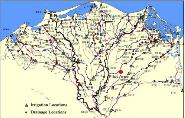
The field work (sampling and measurements) was carried out in MPA. MPA was constructed in 1980 in south-eastern part of the Nile Delta [8]. It is situated 90 km northeast of Cairo in a rather flat area (Figure 1). The area is approximately 260 feddans. Table 1 showed irrigation schedule & amount and crop productiv-ity in MPA, 2005. The layout and design of this pilot area were already planned by the DRI of the National Water Research Center (NWRC), as shown in Figure 1.

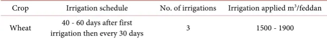
DOI: 10.4236/jwarp.2019.115030 531 Journal of Water Resource and Protection Table 1. Irrigation schedule & amount and crop productivity in MPA, 2005.

Irrigation applied m3_/feddan No. of irrigations

Irrigation schedule Crop

1500 - 1900 3

40 - 60 days after first irrigation then every 30 days Wheat

The southern and western boundaries are formed by the Mahmoudia Drain and its branch; the northern and eastern are bound by tertiary irrigation canals. It is characterized by a deep clay top layer and a sandy aquifer. The clay layer, which is approximately 6.0 m thick, contains about 35% silt and 65% clay. Irrigation water is delivered by gravity to the tertiary canals and lifted approximately 0.5 m to field level by pumps.

The area is drained through a subsurface drainage system that consists of par-allel PVC lateral drains, which discharge into buried concrete collector drains through a manhole. The design of the subsurface drainage system was made ac-cording to the standard criteria of the Egyptian Public Authority for Drainage Projects (EPADP). Two types of criteria can be distinguished; namely, the agri-cultural and the technical ones. The agriagri-cultural criteria are an average depth of the groundwater table midway between the drains of 1.0 m and an average drainage rate of 1.0 mm/day to permit sufficient leaching. The technical criteria are a design discharge rate for the determination of drain pipe capacity of 4 mm/day for rice areas and 3 mm/day for other crops, a safety factor of 25% in the design of the collector drains to account for sedimentation and misalignment and change in diameters and maximum depth of 1.5 m for laterals and 2.5 m for col-lectors. The area was divided into eighteen drainage units with different drain depths and spacing. The units were cultivated with a single crop for each unit during each cropping season. Berseem (Egyptian clover) and wheat were culti-vated as winter crops and cotton, rice, and maize as summer crops [9].

MPA was controlled under the existing farming conditions, aiming to apply the data measurement program for two years, from June 2005 to May 2007, and consequently two winter and two summer seasons. The area was surveyed with a Global Positioning System (GPS) to locate its boundaries, and with a Geographic Information System (GIS) for sampling locations, as shown in Figure 2. The sampling locations included the manholes for field lateral drainage water sam-pling and collectors’ outlets for collector drainage water samsam-pling. The meas-urement program was applied in the area for the four seasons as follows;

 Determination crop pattern, fertilizer amount, and time required to apply each crop for each unit.

 Collected drainage water samples before cultivation, before and after apply-ing fertilizers, and periodically every 10 days.

3. Method and Materials

3.1. Model Development: Conceptual Model

DOI: 10.4236/jwarp.2019.115030 532 Journal of Water Resource and Protection Figure 2. Sampling locations in MPA.

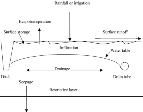
Figure 3. Overview of the main processes included in the conceptual model to calculate the drainage and related water table management.

DOI: 10.4236/jwarp.2019.115030 533 Journal of Water Resource and Protection

3.2. Modelling System

The conceptual model was applied on the study site to model the water balance predictions of the subsurface drainage which is employed to simulate the per-formance of drainage and related water management systems.

The conceptual model uses dynamic modeling to quantify subsurface drain-age, deep seepdrain-age, infiltration, and evapotranspiration. Subsurface drainage flux is calculated based on the assumption that mainly lateral water movement oc-curs in the saturated region. The flux is determined by the water table elevation at the mid plane of the drains and the water level in the drains. The Hooghoudt’s steady-state equation [11] is used when the depth of water on the surface is less than the surface storage (S1):

2

2

8 _{e e dr} 4 _{e dr}

H

rf dr

K d m K m

q

c L

+

= ₍₁₎

where qH is the water flux [L T−1_{], mdr is the midpoint water table height above} the drain [L], Ke is the effective lateral hydraulic conductivity [L T−1_{] and Ldr is} the horizontal distance between drains [L]. de is the equivalent depth from the drain to the restrictive layer [L] and is specified in the model to correct for con-vergence flux near the drains. It can be defined as a function of Ldr, the drainage tube radio rdr [L] and d [L], the real depth from the drain to the restrictive layer [12]. crf is the ratio of the average flux between the drains to the flux midway between the drains and is controlled by the shape of the water table profile. crf is approximated as 1.0, which implies that Equation (1) corresponds to the ellipse equation that is often used to determine drain spacing [12] [13]. Because the soil is not a homogeneous media, Ke is defined as:

( )

(

)

1

1

with 0.0 and for

i N

H i i

i

e i N i P P

i i

K E

K E E d i P

E = = = = =

∑

∑

where N is the number of soil (horizontal) layers, (KH)i is the horizontal hydrau-lic conductivity of the i-th horizontal layer and Ei is the thickness of the i-th layer [L]. This equation should be used observing the convention that soil layers are numbered progressively from up to down. If the water table is located in soil layer P (with 1 ≤ P ≤ N), then dP is the distance between the midpoint water ta-ble elevation and the bottom of layer P.

In the event that the depth of water on the surface exceeds S1 (the surface storage), the assumption of a curved water table completely below the soil sur-face fails (Bouwer and van Schilfgaarde, 1963) and in this case, the flux is calcu-lated as:

(

)

2

4π e pn dr dr

H

pn dr

K z z r

q

c L

+ −

= (3)

DOI: 10.4236/jwarp.2019.115030 534 Journal of Water Resource and Protection drain-size, -depth and -spacing (Skaggs, 1981). The deep vertical seepage flux is computed using Darcy’s law to calculate the flux through the restrictive layer:

(

)

V V

rest

h h q K

E

−

= ₍₄₎

where qv is the deep vertical seepage flux [L T−1_{], KV is the effective vertical} hy-draulic conductivity of the restrictive layer [L T−1_{], h1 is the average distance} from the bottom of the restrictive layer to the water table [L], h2 is the hydraulic head in the groundwater aquifer referenced to the bottom of the restrictive layer [L], and Erest is the thickness of the restrictive layer [L]. Infiltration is computed through a modified Green-Ampt procedure. The potential evapotranspiration (PET) is estimated using the Thornthwaite equation [14].

4. Results and Discussion

Despite the efforts of several alternative approaches to manage intangible fac-tors, none has been sufficient to fully incorporate relationships between va-riables, delays and feedback, all of which characterize the behavior of intangible resources. So, Managers continue taking decisions only based (or support) on their experience, knowledge that constitute their mental models [15] [16]. There-fore, there is a need to explore new tools to represent the complex relationships found in systems. One promising option is system dynamics which is a feed-back-based, object-oriented approach. Although system dynamics is not a novel approach, it offers a new way of modeling for future dynamics of complex sys-tems. According to Simonovic and Fahmy [17], system dynamics is based on a theory of system structure and a set of tools for representing complex systems and analyzing their dynamic behavior. The most important feature of system dynamics is that it helps to elucidate the endogenous structure of the system under consideration, and demonstrate how different elements of a system ac-tually relate to each other. This facilitates experimentation as relations within the system are changed to reflect different decisions [18] [19]. Agricultural systems and their environmental effects, like many other environmental problems, con-stitute complex systems, which study requires systemic approaches capable of explicitly managing the temporal dimension, sustainability conditions, uncer-tainty and externalities [20] [21]. Therefore, the system dynamic is good ap-proach to model this system.

4.1. Causal Loop Diagram

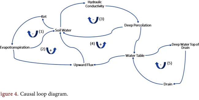
DOI: 10.4236/jwarp.2019.115030 535 Journal of Water Resource and Protection If an initial increase in a variable eventually results in a decreasing effect on the same variable, then the feedback loop is identified as a negative, counteracting or balancing’ loop [22] [23].

The causal loop diagram in this study has shown in Figure 4. The first nega-tive feedback loop represents the evapotranspiration effect: the larger the evapo-transpiration, the less the soil water content and soil moisture stress “ket”, which in turn decreases evapotranspiration. The second feedback loop represents the interaction between evapotranspiration and upward flux: the larger the evapo-transpiration, the larger the upward flux, then the larger the soil water content and ket, which in turn increases evapotranspiration. The third feedback loop represents the interaction between soil water storage and percolation: the larger the storage, the larger the hydraulic conductivity, then the larger the percolation, which in turn decreases soil water storage. The fourth feedback loop represents interaction between water table and soil water storage: an increase in the perco-lation increases water table and upward flux and soil water content. In the fifth feedback loop as water table rises by deep percolation, the depth of water above the drain increases which increases the drain discharge, and in turn decreases the water table.

4.2. Model Calibration

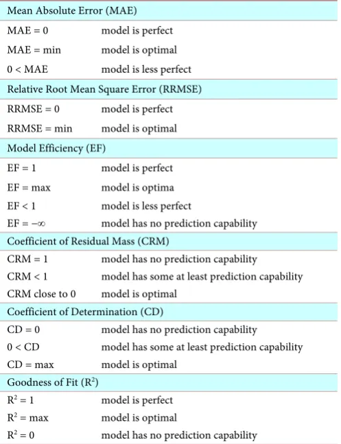
The model was calibrated by considering the time series of observed subsurface flux at the outlet of the drainage system (Figure 5). The calibration was carried out through a trial and error approach by which the parameters were varied manually on the basis of the assessment of model performance. Model perform-ance evaluation was based on visual inspection of calibration plots (hydrographs of observed and predicted time series, hydrographs of observed and predicted cumulative time series, scatter plots of observed and predicted time series, etc.) and on the statistical assessment of model performance indexes such as; Mean Absolute Error (MAE), Relative Root Mean Square Error (RRMSE), Model Effi-ciency (EF), Coefficient of Residual Mass (CRM), Coefficient of Determination (CD) and, Goodness of Fit (R2_{). The characteristic of the different statistical} cri-teria is given in Table 2.

DOI: 10.4236/jwarp.2019.115030 536 Journal of Water Resource and Protection Figure 5. Measured and simulated subsurface drainage water under wheat crop in a MPA using Stella dynamic modelling.

Table 2. The characteristic of the different statistical criteria. Mean Absolute Error (MAE)

MAE = 0 model is perfect

MAE = min model is optimal

0 < MAE model is less perfect Relative Root Mean Square Error (RRMSE)

RRMSE = 0 model is perfect

RRMSE = min model is optimal Model Efficiency (EF)

EF = 1 model is perfect

EF = max model is optima

EF < 1 model is less perfect

EF = −∞ model has no prediction capability Coefficient of Residual Mass (CRM)

CRM = 1 model has no prediction capability CRM < 1 model has some at least prediction capability CRM close to 0 model is optimal

Coefficient of Determination (CD)

CD = 0 model has no prediction capability

0 < CD model has some at least prediction capability

CD = max model is optimal

Goodness of Fit (R2₎

R2 _{= 1 model is perfect}

R2 _{= max model is optimal}

R2 _{= 0 model has no prediction capability}

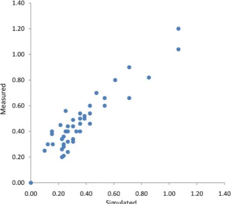
DOI: 10.4236/jwarp.2019.115030 537 Journal of Water Resource and Protection Figure 6. Measured and simulated subsurface drainage water in a MPA.

Table 3. Statistical analysis results of water table in MPA.

MAE RRMSE CD EF CRM R2

Measured & Dynamic system 0.450 0.344 0.780 0.821 0.133 0.873

MAE: mean absolute error; RRMSE: relative root mean square error; CD: coefficient of determination; EF: model efficiency; CRM: coefficient of residual mass; R2_{: goodness of fit.}

5. Conclusion

A dynamic model was developed to predict drain discharge behavior for differ-ent drain systems (depth and spacing). The developed model was used to simu-late the daily drainage water at the midpoint of drain spacing in a clay soil. The measured data and simulated results were compared in terms of subsurface drainage discharge. The statistical analysis implies a good fit between measured and simulated values. The comparative study reveals that the model performs well, reliable and accurate for predicting subsurface drainage water in clay soils. Results (predictions) can be used to design the drainage system geometry for better water management on both field and catchment scales. Results indicated that, the model can be used as a decision support tool to help policy makers in long term strategic management for irrigation projects. The developed model can potentially help in setting guidelines for using subsurface drainage water in agricultural sector in Egypt.

Conflicts of Interest

The authors declare no conflicts of interest regarding the publication of this pa-per.

References

DOI: 10.4236/jwarp.2019.115030 538 Journal of Water Resource and Protection Drain Flow and Crop Yield Predictions for Different Drain Spacings Using DRAINMOD.Agricultural Water Management,79, 113-136.

https://doi.org/10.1016/j.agwat.2005.02.002

[2] El-Sadek, A., Feyen, J. and Berlamont, J. (2001) Comparison of Models for Com-puting Drainage Discharge. Irrigation and Drainage Engineering, 127, 363-369.

https://doi.org/10.1061/(ASCE)0733-9437(2001)127:6(363)

[3] Filipović, V., Mallmann, F.J.K., Coquet, Y. and Šimůnek, J. (2014) Numerical Simu-lation of Water Flow in Tile and Mole Drainage Systems. Agricultural Water Man-agement, 146, 105-114.https://doi.org/10.1016/j.agwat.2014.07.020

[4] El-Sadek, A., Oorts, K., Sammels, L., Timmerman, A., Radwan, M. and Feyen, J. (2003) Comparative Study of Two Nitrogen Models. Irrigation and Drainage Engi-neering, 129, 44-52.https://doi.org/10.1061/(ASCE)0733-9437(2003)129:1(44)

[5] Haan, P. (2000) The Effect of Parameter Uncertainty on DRAINMOD Predictions for Hydrology, Yield and Water Quality. Doctoral Dissertation, Biological and Agricultural Engineering Department, North Carolina State University, Raleigh, 153.

[6] Haan, P.K. and Skaggs, R.W. (2003) Effect of Parameter Uncertainty on DRAINMOD Predictions: I. Hydrology and Yield. Transactions of the ASAE, 46, 1061-1067. [7] Forrester, J.W. (1968) Principles of Systems. Productivity Press, Cambridge, MA. [8] Drainage Research Institute (DRI) (1987) Mashtul Pilot Area, Physical Description.

Technical Report No. 57, Pilot Areas and Drainage Technology Project, Drainage Research Institute, Cairo.

[9] El-Sadek, A., Sallam, G. and Embaby, M (2013) Using DRAINMOD-Geostatistical Technology to Predict Nitrate Leaching: A Case Study of Mashtul Pilot Area, Egypt.

Irrigation and Drainage Engineering, 139, 158-164.

https://doi.org/10.1061/(ASCE)IR.1943-4774.0000491

[10] van Genuchten, M.Th. (1980) A Closed-Form Equation for Predicting the Hydrau-lic Conductivity of Unsaturated Soils. Soil Science Society of America Journal, 44, 892-898.https://doi.org/10.2136/sssaj1980.03615995004400050002x

[11] Bouwer, H. and van Schilfgaarde, J. (1963) Simplified Method of Predicting the Fall of Water Table in Drained Land. Transactions of the ASAE, 6, 288-291.

https://doi.org/10.13031/2013.40893

[12] Skaggs, R.W. (1981) Methods for Design and Evaluation of Drainage Water Man-agement Systems for Soils with High Water Tables, DRAINMOD. North Carolina State University, Raleigh, North Carolina.

https://www.bae.ncsu.edu/agricultural-water-management/drainmod/drainmod-pu blications/#development

[13] El-Sadek, A. and Vazquez, R. (2012) Parameter Sensitivity Analysis and Prediction error in Field-Scale NO3-N Modeling. Agricultural Water Management, 111, 115-126. https://doi.org/10.1016/j.agwat.2012.05.010

[14] Thornthwaite, C.W. (1948) An Approach toward a Rational Classification of Cli-mate. Geographical Review, 38, 55-94.https://doi.org/10.2307/210739

[15] Ortiz, A., Sarriegui, J. and Santos, J. (2006) Applying Modelling Paradigms to ana-lyse Organisational Problems. 7th System Dynamics PhD Colloquium 23rd, Nijme-gen, 23-27 July 2006, 1-18.

Dy-DOI: 10.4236/jwarp.2019.115030 539 Journal of Water Resource and Protection namics Approach. Ecological Modelling, 347, 11-28.

https://doi.org/10.1016/j.ecolmodel.2016.12.014

[17] Simonovic, S.P. and Fahmy, H. (1999) A New Modelling Approach for Water Re-sources Policy Analysis. Water Resources Research, 35, 295-304.

https://doi.org/10.1029/1998WR900023

[18] Elmahdi, A., Malano, H., Etchells, T. and Khan, S. (2005) System Dynamics Opti-misation Approach to Irrigation Demand Management. In: Zerger, A. and Argent, R.M., Eds., MODSIM 2005 International Congress on Modelling and Simulation, Modelling and Simulation Society of Australia and New Zealand, 196-202.

[19] Sušnik, J., Molina, J.L., Vamvakeridou-Lyroudia, L.S., Savić, D.A. and Kapelan, Z. (2013) Comparative Analysis of System Dynamics and Object-Oriented Bayesian Networks Modelling for Water Systems Management. Water Resources Manage-ment, 27, 819-841.https://doi.org/10.1007/s11269-012-0217-8

[20] Nozari, H. and Liaghat, A. (2014) Simulation of Drainage Water Quantity and Quality Using System Dynamics. Journal of Irrigation and Drainage Engineering, 140, 1943-4774.https://doi.org/10.1061/(ASCE)IR.1943-4774.0000748

[21] Liu, H., Benoit, G., Liu, T., Liu, Y. and Guo, H. (2015) An Integrated System Dy-namics Model Developed for Managing Lake Water Quality at the Watershed Scale.

Journal of Environmental Management, 155, 11-23.

https://doi.org/10.1016/j.jenvman.2015.02.046

[22] Saysel, A.K. and Barlas, Y. (2001) A Dynamic Model of Stalinization on Irrigated Lands. Ecological Modeling, 139, 177-199.

https://doi.org/10.1016/S0304-3800(01)00242-3