A Logical Framework for Reputation Systems

A Logical Framework for Reputation Systems

Karl Krukow

BRICS

University of Aarhus, Denmark

[email protected]

Mogens Nielsen

BRICS

University of Aarhus, Denmark

[email protected]

Vladimiro Sassone

Department of Informatics

University of Sussex, UK

[email protected]

4th January 2006

Abstract

Reputation systems are meta systems that record, aggregate and dis-tribute information about the past behaviour of principals in an applica-tion. Typically, these applications are large-scale open distributed systems where principals are virtually anonymous, and (a priori) have no knowl-edge about the trustworthiness of each other. Reputation systems serve two primary purposes: helping principals decide whom to trust, and pro-viding an incentive for principals to well-behave.

A logical policy-based framework for reputation systems is presented. In the framework, principals specify policies which state precise require-ments on the past behaviour of other principals that must be fulfilled in order for interaction to take place. The framework consists of a formal model of behaviour, based on event structures; a declarative logical lan-guage for specifying properties of past behaviour; and efficient dynamic algorithms for checking whether a particular behaviour satisfies a property from the language. It is shown how the framework can be extended in several ways, most notably to encompass parameterized events and quan-tification over parameters. In an extended application, it is illustrated how the framework can be applied for dynamic history-based access control for safe execution of unknown and untrusted programs.

Keywords. Reputation systems, history-based access control, trust manage-ment, dynamic model checking, event structures, linear temporal logic.

1

Introduction

Rich opportunities for fraud exist on the Internet. Still, risky interactions like electronic commerce, involving disclosure of private informations to semi-trusted parties, are every-day activities in our Internet lives. It seems that in practice, for most people, the utility of the Internet outweighs its risks. When one tries to understand better these facts, mathematical models from economic theory are very appealing. Online interaction can often be seen as a ‘repeated game’ played between selfish (semi) rational principals. Such interaction may result in utility gains for the involved principals, but often, with interaction comes also an associated inherent risk; a potential utility-loss. For risk-adverse principals, the fear of loss may outweigh the expectation of gain, leading to an unwillingness to participate. For example, one might have expected that an online auctioning system such as eBay, “a market ripe with the possibility of large-scale fraud and deceit” [19], would never have reached the more than one million transactions per day that are presently processed. The liveness on eBay is often attributed to its so-called Feedback Forum, a simple example of a reputation system. When principals have transacted, each party may leave feedback on the eBay web-site, consisting of a rating of ‘positive’, ‘neutral’ or ‘negative’. A principal’s aggregated rating is then visible to potential buyers or sellers before deciding whether to interact or not. In general, reputation systems record, aggregate and (sometimes) distribute information about the past behaviour of principals. Hence reputation systems may serve as a trust-enabling, or perhaps, more gen-erally, trust-informing technology. Resnick et al. argue that reputation systems foster an incentive for principals to well-behave because of “the expectation of reciprocity or retaliation in future interactions” [28], and reputation itself has previously been formalized and analyzed by economists in simple game-theoretic models, leading to similar conclusions (e.g., [6,7,20,36]); it seems that reputation systems are well etablished, and their is usefulness generally accepted.

further in the concluding section.

Abstract representations of behavioural information have their advantages (e.g., numerical values are often easily comparable, and require little space to store), but clearly, information is lost in the abstraction process. For example, in EigenTrust, value ‘0’ may represent both “no previous interaction” and “many unsatisfactory previous interactions”[17]. Consequently, one cannot verify exact properties of past behaviour given only the reputation information.

In this paper, the concept of ‘reputation system’ is to be understood very broadly, simply meaningany system in which principals record and use infor-mation about past behaviour of principals, when assessing the risk of future interaction. Aprincipal is simply an identity; it may be the identity of a human users, a public key, a software program (e.g., an identifiable instance), etc. We present a formal framework for a class of simple reputation systems in which, as opposed to most “traditional”systems, behavioural information is represented in a very concrete form. The advantage of our concrete representation is that suffi-cient information is present to check precise properties of past behaviour. In our framework, such requirements on past behaviour are specified in a declarative policy-language, and the basis for making decisions regarding future interaction becomes the verification of a behavioural history with respect to a policy. This enables us to define reputation systems that provide a form of provable “secu-rity” guarantees, intuitively, of the form: “If principalpgains access to resource

rat time t, then the past behaviour of pup until timet satisfies requirement

ψr.”

To get the flavour of such requirements, we preview an example policy from a declarative language formalized in the following sections. Edjlali et al. [9] consider a notion of history-based access control in which unknown programs, in the form of mobile code, are dynamically classified into equivalence classes of programs according to their behaviour (e.g. “browser-like” or “shell-like”). This dynamic classification falls within the scope of our very broad understanding of reputation systems. The following is an example of a policy written in our language, which specifies a property similar to that of Edjlali et al., used to classify “browser-like” applications:

ψ ≡ ¬F−1_{(modify-file) ∧}

¬F−1_{(create-subprocess) ∧}

G−1 _∀x.

open(x)→F−1_(create(x))

Informally, the atomsmodify-file,create-subprocess,open(x) andcreate(x) areeventswhich are observable by monitoring an entity’s behaviour. The latter two areparameterized events, and the quantification “∀x” ranges over the pos-sible parameters of these. OperatorF−1_{means ‘at some point in the past,’G}−1 means ‘always in the past,’ and constructs∧and¬are conjunction and negation, respectively. Thus, clauses¬F−1_{(modify-file) and¬F}−1_{(create-subprocess)} require that the application has never modified a file, and has never created a sub-process. The final, quantified clauseG−1 _∀x.

”/etc/passwd” (i.e. a file which it has not created) then it cannot access the network (a right assigned to the “browser-like” class). If, instead, the applica-tion has previously only read files it has created, then it will be allowed network access.

1.1

Contributions and Outline

We present a formal model of the behavioural information that principals ob-tain in our class of reputation systems. This model is based on previous work using event structures [37] for modelling observations [25], but our treatment of behavioural information departs from the previous work in that we perform (almost) no information abstraction. The event-structure model is presented in Section 2.

We describe our formal declarative language for interaction policies. In the framework of event structures, behavioural information is modelled as sequences of sets of events. Such linear structures can be thought of as (finite) models of linear temporal logic (LTL) [26]. Indeed, our basic policy language is based on a (pure-past) variant of LTL. We give the formal syntax and semantics of our language, and provide several examples illustrating its naturality and expres-siveness. We are able to encode several existing approaches to history-based access control, e.g. the Chinese Wall security policy [2] and a restricted ver-sion of so-called ‘one-out-of-k’ access control [9]. The formal description of our language, as well as examples and encodings, is presented in Section 3.

An interesting new problem is how to re-evaluate policies efficiently when interaction histories change as new information becomes available. It turns out that this problem, which can be described as dynamic model-checking, can be solved very efficiently using an algorithm adapted from that of Havelund and Ro¸su, based on the technique of dynamic programming, used for runtime verification [13]. Interestingly, although one is verifying properties of anentire

interaction history, one needs not store this complete history in order to verify a policy: old interaction can be efficiently summarized relative to the policy. In Section 4, two dynamic algorithms for policy checking is described, analysed and compared.

of most existing reputation systems. Another common characteristic is focus on conveying quantitative information. In contrast, standard temporal logic is qualitative: it deals with concepts such asbefore, after,always and eventually. We show that we can extend our language to include a range of quantitative aspects, intuitively, operators like ‘almost always,’ ‘more thanN,’ etc. Section 5 illustrates these two extensions, and briefly discusses policy-checking for the extended languages.

Throughout the paper, we have small examples illustrating the applicability of our framework within the area of history-based access control. We have taken this one step further by developing a prototype security manager for Java, based on our logical framework. The security manager is parameterized by a policy in our language, and monitors a Java program with respect to this policy, throwing an exception if a violation is about to happen. In Section 6, we describe this application of our framework to history-based access control for Java programs. Related work is discussed in the concluding section.

2

Observations as Events

Agents in a distributed system obtain information by observing events which are typically generated by the reception or sending of messages. The structure of these message exchanges are given in the form of protocols known to both parties before interaction begins. By behavioural observations, we mean observations that the parties can make about specific runs of such protocols. These include information about the contents of messages, diversion from protocols, failure to receive a message within a certain time-frame, etc.

Our goal in this section, is to give precise meaning to the notion of be-havioural observations. Note that, in the setting of large-scale distributed en-vironments, often, a particular agent will (concurrently) be involved in several instances of protocols; each instance generating events that are logically con-nected. One way to model the observation of events is using a process algebra with “state”, recording input/output reactions, as is done in the calculus for trust management, ctm _{[5]. Here we are not interested in modelling}

interac-tion protocols in such detail, but merely assume some system responsible for generating events.

We present the event-structure framework as an abstract interface providing two operations,newandupdate, which respectively records the initiation of a new protocol run, and updates the information recorded about an older run (i.e. updates an event-setxi). A specific implementation then uses this interface to notify our framework about events.

2.1

The Event Structure Framework

In order to illustrate the event-structure framework, we use an example comple-menting its formal definitions. We will use a scenario inspired by the eBay online auction-house [8], but deliberately over-simplified to illustrate the framework.

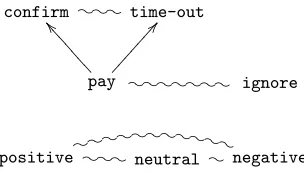
On the eBay website, a seller starts an auction by announcing, via the web-site, the item to be auctioned. Once the auction has started the highest bid is always visible, and bidders can place bids. A typical auction runs for 7 days, after which the bidder with the highest bid wins the auction. Once the auction has ended, the typical protocol is the following. The buyer (winning bidder) sends payment of the amount of the winning bid. When payment has been received, the seller confirms the reception of payment, and ships the auctioned item. Optionally, both buyer and seller may leave feedback on the eBay site, expressing their opinion about the transaction. Feedback consist of a choice between ratings ‘positive’, ‘neutral’ and ‘negative’, and, optionally, a comment. We will model behavioural information in the eBay scenario from the buyers point of view. We focus on the interaction following a winning bid, i.e. the protocol described above. After winning the auction, buyer (B) has the option to send payment, or ignore the auction (possibly risking to upset the seller). If

Bchooses to send payment, he may observe confirmation of payment, and later the reception of the auctioned item. However, it may also be the case that B

doesn’t observe the confirmation within a certain time-frame (the likely scenario being that the seller is a fraud). At any time during this process, each party may choose to leave feedback about the other, expressing their degree of satisfaction with the transaction. In the following, we will model an abstraction of this scenario where we focus on the following events: buyer pays for auction, buyer ignores auction, buyer receives confirmation, buyer receives no confirmation within a fixed time-limit, andseller leaves positive, neutral or negative feedback (note that we do not model thebuyer leaving feedback).

(e.g., it doesnot mean that the events are independent in any statistical sense). These relations between observations are directly reflected in the definition of an event structure. (For a general account of event structures [37], traditionally used in semantics of concurrent languages, consult the handbook chapter of Winskel and Nielsen [38]).

Definition 2.1 (Event Structure). An event structure is a triple ES = (E,≤,#) consisting of a setE, and two binary relations onE: ≤and #. The elementse∈Eare calledevents, and the relation #, called theconflict relation, is symmetric and irreflexive. The relation ≤is called the (causal) dependency relation, and partially ordersE. The dependency relation satisfies the following axiom, for anye∈E:

the setdee(def)= {e0∈E|e0 ≤e}is finite.

The conflict- and dependency-relations satisfy the following “transitivity” axiom for anye, e0_{, e}00_∈E

e#e0 ande0≤e00

impliese# e00

Two events areindependent if they are not in either of the two relations.

We use event structures to model the possible observations of a single agent in a protocol, e.g. the event structure in Figure 1 models the events observable by the buyer in our eBay scenario.

The two relations on event structures imply that not all subsets of events can be observed in a protocol run. The following definition formalizes exactly what sets of observations are observable.

Definition 2.2 (Configuration). LetES= (E,≤,#) be an event structure. We say that a subset of eventsx⊆Eis aconfigurationif it isconflict free(C.F.), andcausally closed (C.C.). That is, it satisfies the following two properties, for anyd, d0_∈xande∈E

(C.F.) dr_#d0_{; and (C.C.)e≤d⇒e∈x}

Notation 2.1. CES denotes the set of configurations ofES, and CES0 ⊆ CES

the set of finite configurations. A configuration is said to be maximal if it is maximal in the partial order (CES,⊆). Also, if e∈ E and x ∈ CES, we write e# x, meaning that ∃e0 _{∈x.e # e}0_{. Finally, for x, x}0 _{∈ CES, e∈ E, define a}

relation→byx→e x0 _{iffe6∈x andx}0 _{=x∪ {e}. If y⊆E andx∈ CES, e∈E}

we writex6→e yto mean that eithery6∈ CES or it is not the case thatx e

→y.

A finite configuration models information regardinga single interaction, i.e. a single run of a protocol. A maximal configuration represents complete infor-mation about a single interaction. In our eBay example, sets∅,{pay,positive}

and{pay,confirm,positive}are examples of configurations (the last configu-ration being maximal), whereas

and{confirm}are non-examples.

In general, the information that one agent possesses about another will con-sist of information about several protocol runs; the information about each individual run being represented by a configuration in the corresponding event structure. The concept of a local interaction history models this.

Definition 2.3 (Local Interaction History). LetESbe an event structure, and define alocal interaction history in ES to be a sequence of finite configu-rations,h=x1x2· · ·xn ∈ CES0

∗

. The individual componentsxi in the historyh

will be calledsessions.

In our eBay example, a local interaction history could be the following:

{pay,confirm,pos}{pay,confirm,neu}{pay}

Here pos and neu are abbreviations for the events positive and neutral. The example history represents that the buyer has won three auctions with the particular seller, e.g. in the third session the buyer has (so-far) observed only eventpay.

We assume that the actual system responsible for notification of events will use the following interface to the model.

Definition 2.4 (Interface). Define an operation new : C0

ES

∗ → C0

ES

∗

by new(h) =h∅. Define also a partial operation update:C0

ES

∗

×E×N→ C0

ES

∗

as follows. For anyh=x1x2· · ·xi· · ·xn ∈ CES0

∗

, e∈E,i∈N_{,update(h, e, i)}

is undefined ifi6∈ {1,2, . . . , n}or xi6→e xi∪ {e}. Otherwise

update(h, e, i) =x1x2· · ·(xi∪ {e})· · ·xn

Remarks. The notion of time in the model is based on when sessions are

started. More precisely, in our local interaction histories,h=x1x2· · ·xn where

xi∈ CES, the order of the sessions reflectsthe order in which the corresponding

interaction-protocols are initiated, i.e. xi refers to the observed events in the

ith-initiated session. Different notions of time could just as well be considered, e.g. ifxi precedesxj in sequence h, then it means thatxj was updated more recently thanxi.

Note, while the order of sessions is recorded (a local history is asequence), in contrast, the order ofindependent events withina single session is not. For example, in our eBay scenario we have

update(update({pay},neutral,1),confirm,1) = update(update({pay},confirm,1),neutral,1)

use a “serialized” event structure in which this order of occurrences is recorded. A serialization of events consists of splitting the events in question into different events depending on the order of occurrence, e.g., supposing in the example one wants to record the order of payand pos, one replaces these events with eventspay-before-pos,pos-before-pay,pay-after-posandpos-after-pay

with the obvious causal- and conflict-relations.

When applying our logic (described in the next section) to express policies for history-based access control (HBAC), we use a special type of event structure in which the conflict relation is the maximal irreflexive relation on a setEof events. The reason is thathistories in many frameworks for HBAC, are sequences of single events for a set E. When the conflict relation is maximal on E, the configurations of the corresponding event structure are exactly singleton event-sets, hence we obtain a useful specialization of our model, compatible with the tradition of HBAC.

3

A Language for Policies

The reason for recording behavioural information is that it can be used to guide future decisions about interaction. We are interested in binary decisions, e.g., access-control and deciding whether to interact or not. In our proposed system, such decisions will be made according to interaction policies that specify exact requirements on local interaction histories. For example, in the eBay scenario from last section, the bidder may adopt a policy stating: “only bid on auctions run by a seller which has never failed to send goods for won auctions in the past.” Notice, by the way, that users would have a hard time implementing such a policy using the current eBay feedback forum.

In this section, we propose a declarative language which is suitable for speci-fying interaction policies. In fact, we shall use a pure-past variant of linear-time temporal logic, a logic introduced by Pnueli for reasoning about parallel pro-grams [26]. Pure-past temporal logic turns out to be a natural and expressive language for stating properties of past behaviour. Furthermore, linear-temporal-logic models are linear Kripke-structures, which resemble our local interaction histories. We define a satisfaction relation|=, between such histories and poli-cies, where judgementh|=ψmeans that the historyhsatisfies the requirements of policyψ.

3.1

Formal Description

3.1.1 Syntax.

The syntax of the logic is parametric in an event structure ES= (E,≤,#). There are constant symbols for each e ∈ E (ranged over by meta-variables

e, e0_{, ei, . . .). The syntax of our language, which we denote L(ES), is given by}

the following BNF.

The constructseand3eare bothatomicpropositions. In particular,3eisnot

the application of the usual modal operator3(with the “temporal” semantics) to formula e. Informally, the formula e is true in a session if the evente has been observed in that session, whereas3e, pronounced “eis possible”, is true if eventemay still occur as a future observation in that session. The operators

X−1_{(‘last time’) and S (‘since’) are the usual past-time operators.}

3.1.2 Semantics.

Astructure forL(ES), whereES = (E,≤,#) is an event structure, is a non-empty local interaction history in ES, h ∈ C0

ES

+

. We define the satisfaction relation|= between structures and policies, i.e.h|=ψmeans that the historyh

satisfies the requirements of policyψ. We will use a variation of the semantics in linear Kripke structures: satisfaction is defined from theend of the sequence “towards” the beginning, i.e. h |= ψ iff (h,|h|) |= ψ. To define the semantics

of (h, i) |= ψ, let h = x1x2· · ·xN ∈ CES0

∗

, and i ∈ N_{. Define (h, i)} |= ψ by structural induction inψ.

(h, i)|=e iff 1≤i≤N ande∈xi

(h, i)|=3e iff 1≤i≤N⇒e r_#xi

(h, i)|=ψ0∧ψ1 iff (h, i)|=ψ0and (h, i)|=ψ1 (h, i)|=¬ψ iff (h, i)6|=ψ

(h, i)|=X−1_{ψ iff i >1 and (h, i−1)|=ψ} (h, i)|=ψ0 Sψ1 iff ∃j≤i.(h, j)|=ψ1 and

∀k.(j < k≤i⇒(h, k)|=ψ0)

Remarks. There are two main reasons for restricting ourselves to the pure-past fragment of temporal logic (PPLTL). Most importantly, PPLTL is an ex-pressive andnatural language for stating requirements overpastbehaviour, e.g. history-based access control. Hence in our application one wants to speak about the past, not the future. We justify this claim further by providing (natural) encodings of several existing approaches for checking requirements of past be-haviour (c.f. Example 3.2 and 3.3 in the next section). Secondly, although one could add future operators to obtain a seemingly more expressive language, a result of Laroussinieet al.quantifies exactly what is lost by this restriction [21]. Their result states that LTL can beexponentially more succinct than the pure-future fragment of LTL. It follows from the duality between the pure-pure-future and pure-past operators, that when restricting to finite linear Kripke structures, and interpretingh|=ψas (h,|h|)|=ψ, then our pure-past fragment can expressany

Note that the logic cannot distinguish the empty structure ∈ C∗

ES from a

structure consisting of any number of empty configurations, e.g.,∅∅∅. More gen-erally, one way of looking at our structures is asinfinitesequencesx1x2· · ·xn∅∅ · · ·, having only finitely many non-empty configurations.

We define standard abbreviations using syntatic equality: false_{≡e ∧ ¬efor}

some fixede∈E,true_{≡ ¬}false_{,ψ0∨ψ1≡ ¬(¬ψ0∧ ¬ψ1),ψ0→ψ1≡ ¬ψ0∨ψ1,} F−1_{(ψ) ≡true S ψ, G}−1_{(ψ) ≡ ¬F}−1_{(¬ψ). Note that, F}−1_{(ψ) means “formula}

ψ is true at some time in the past,” whereas G−1_{(ψ) means “ψ is true at all}

times in the past.” We also define a non-standard abbreviation ∼e ≡ ¬3e

(pronounced ‘conflicte’ or ‘eis impossible’).

3.2

Example Policies

To illustrate the expressive power of our language, we consider a number of example policies.

Example 3.1 (eBay). Recall the eBay scenario from Section 2, in which a buyer has to decide whether to bid on an electronic auction issued by a seller. We express a policy for decision ‘bid_{’, stating “only bid on auctions run by a}

seller that has never failed to send goods for won auctions in the past.”

ψbid_{≡ ¬F}−1₍

time-out)

Furthermore, the buyer might require that “the seller has never provided nega-tive feedback in auctions where payment was made.” We can express this by

ψbid_{≡ ¬F}−1₍

time-out)∧G−1₍

negative→ignore)

Example 3.2 (Chinese Wall). The Chinese Wall policy is an important com-mercial security-policy [2], but has also found applications within computer sci-ence. In particular, Edjlaliet al.[9] use an instance of the Chinese Wall policy to restrict program accesses to database relations. The Chinese Wall security-policy deals with subjects (e.g. users) and objects (e.g. resources). The objects are organized into datasets which, in turn, are organized in so-called conflict-of-interest classes. There is a hierarchical structure on objects, datasets and classes, so that each object has a unique dataset which, in turn, has a unique class. In the Chinese-Wall policy, any subject initially has freedom to access any object. After accessing an object, the set of future accessible objects is restricted: the subject can no longer access an object in the same conflict-of-interest class unless it is in a dataset already accessed. Non-conflicting classes may still be accessed.

We now show how our logic can encode any instance of the Chinese Wall policy. Following the model of Breweret al.[2], we letSdenote a set ofsubjects,

datasets and classes amounts to requiring that for anyo, o0_{∈O ifL(o) = (c, d)}

and L(o0_{) = (c}0_{, d) then c = c}0_{. The following ‘simple security rule’ defines}

when access is granted to an object o: “either it has the same dataset as an object already accessed by that subject, or, the object belongs to a different conflict-of-interest class.” [2] We can encode this rule in our logic. Consider an event structure ES = (E,≤,#) where the events are C∪D, with (c, c0_{)∈ #}

for c 6= c0 _{∈ C, (d, d}0_{) ∈ # ford 6= d}0 _{∈ D, and (c, d)∈ # if (c, d) is not in}

the image of L(denotedImg(L)). We take≤to be discrete. Then a maximal configuration is a set{c, d}so that the pair (c, d)∈Img(L), corresponding to an object access. A history is then a sequence of object accesses. Now stating the simple security rule as a policy is easy: to access objectowith L(o) = (co, do), the history must satisfy the following policy:

ψo≡F−1_do∨G−1_¬co

In this encoding we have one policy per object o. One may argue that the policyψo_{only captures Chinese Wall for a single object (o), whereas the “real”}

Chinese Wall policy isa single policy stating that “for every object o, the simple security rule applies.” However, in practical terms this is inessential. Even if there are infinitely many objects, a system implementing Chinese Wall one could easily be obtained using our policies as follows. Say that our proposed security mechanism (intended to implement “real” Chinese Wall) gets as input the object o and the subject s for which it has to decide access. Assuming that our mechanism knows function L, it does the following. If object o has never been queried before in the run of our system, the mechanism generates “on-the-fly” a new policy ψo _{according to the scheme above; it then checksψ}o

with respect to the current history ofs.1 _{Ifo has been queried before it simply} checksψo_{with respect to the history ofs. Since only finitely many objects can}

be accessed in any finite run, only finitely many different policies are generated. Hence, the described mechanism is operationally equivalent to Chinese Wall.

Example 3.3 (Shallow One-Out-of-k). The ‘one-out-of-k’ (OOok) access-control policy was introduced informally by Edjlali et al. [9]. Set in the area of access control for mobile code, the OOok scheme dynamically classifies pro-grams into equivalence classes, e.g. “browser-like applications,” depending on their past behaviour. In the following we show that, if one takes theset-based

formalization of OOok by Fong [11], we can encode all OOok policies. Since our model is sequence-based, it is richer than Fong’s shallow histories which are sets. An encoding of Fong’s OOok-model thus provides a good sanity-check as well as adeclarative means of specifying OOokpolicies (as opposed to the more implementation-oriented security automata).

In Fong’s model of OOok, a finite number of application classes are con-sidered, say, 1,2, . . . , k. Fong identifies an application class, i, with a set of allowed actions Ci. To encode OOok policies, we consider an event structure

ES= (E,≤,#) with eventsEbeing the set of all access-controlled actions. As

1

in the last example, we take ≤ to be discrete, and the conflict relation to be the maximal irreflexive relation, i.e. a local interaction history inES is simply a sequence of single events. Initially, a monitored entity (originally, a piece of mobile code [9]) has taken no actions, and its history (which is a set in Fong’s formalization) is ∅. If S is the current history, then action a ∈ E is allowed if there exists 1≤i ≤k so that S∪ {a} ⊆Ci, and the history is updated to

S∪ {a}. For each actiona∈E we define a policyψa _{fora, expressing Fong’s}

requirement. Assume, without loss of generality, that the setsCj that contain

aare named 1,2, . . . , ifor somei≤k. We will assume that each setCj is either finite or co-finite.

Fix aj ≤i. If the setCj is co-finite (i.e., its complement E\Cj is finite), the following formulaψa

j encodes the requirement thatS∪ {a} ⊆Cj.

ψja≡ ¬F−1(

_

e∈E\Cj

e)

If insteadCj is itself finite, we encode

ψa

j ≡G−1(

_

e∈Cj

e)

Now we can encode the policy for allowing actionaasψa≡Wi

j=1ψaj.

4

Dynamic Model Checking

The problem of verifying a policy with respect to a given observed history is the model-checking problem: givenh∈ C_ES+ andψ, doesh|=ψhold? However, our intended scenario requires a more dynamic view. Each entity will make many decisions, and each decision requires a model check. Furthermore, since the model hchanges as new observations are made, it is not sufficient simply to cache the answers. This leads us to consider the followingdynamic problem. Devise an implementation of the following interface, ‘DMC’. DMC is initially given an event structure ES = (E,≤,#) and a policy ψ written in the ba-sic policy language. Interface DMC supports three operations: DMC.new(),

DMC.update(e, i), and DMC.check(). A sequence of non-‘check’ operations gives rise to a local interaction historyh, and we shall call this the actual his-tory. Internally, an implementation ofDMC must maintain information about the actual history h, and operationsnew and updateare those of Section 2, performed onh. At any time, operationDMC.check() must return the truth ofh|=ψ.

LTL [13]. Their idea is essentially this: because of the recursive semantics, model-checkingψ in (h, m), i.e. deciding (h, m)|=ψ, can be done easily if one knows (1) the truth of (h, m−1) |= ψj for all sub-formulas ψj of ψ, and (2) the truth of (h, m)|=ψi for all proper sub-formulasψi of ψ (a sub-formula of

ψ is proper if it is not ψ itself). The truth of the atomic sub-formulas of ψ

in (h, m) can be computed directly from the state hm, where hm is the mth configuration in sequenceh. For example, ifψ3=X−1ψ4∧e, then (h, m)|=ψ3 iff (h, m−1)|=ψ4, ande∈hm. This information needed to decide (h, m)|=ψ

can be stored efficiently as two boolean arraysBlast and Bcur, indexed by the sub-formulas ofψ, so thatBlast[j] is true iff (h, m−1)|=ψj, andBcur[i] is true iff (h, m)|=ψi. Given arrayBlast and the current statehm, one then constructs arrayBcur starting from the atomic formulas (which have the largest indices), and working in a ‘bottom-up’ manner towards index 0, for which entryBcur[0] represents (h, m)|=ψ. We shall generalize this idea of Havelund and Ro¸su to obtain an algorithm for the dynamic problem.

We need some preliminary terminology. Initially, the actual interaction his-tory h is empty, but after some time, as observations are made, the history can be writtenh=x1·x2· · ·xM ·yM+1· · ·yM+K, consisting of alongest prefix x1· · ·xM of maximal configurations, followed by a suffix of K possibly non-maximal configurationsyM+1· · ·yM+K, called theactivesessions (since we

con-sider the longest prefix,yM+1must be non-maximal). A maximal configuration represents complete information about a protocol-run, and has the property that it will never change in the future, i.e. cannot be changed by operationupdate. This property will be essential to our dynamic algorithms as it implies that the maximal prefix needs not be stored to checkh|=ψ dynamically.

In the following, the numberM will always refer to the size of the maximal prefix, andKto the size of the suffix.

4.1

An Array-based Implementation

We describe an implementation of theDMC interface based on a data structure

DS maintaining the active sessions and a collection of boolean arrays. Under-standing the data structure is underUnder-standing the invariant it maintains, and we will describe this in the following.

The data structure DS has a vector, accessed by variable DS.h, storing configurations of ES, which we denote DS.h = (y1, y2, . . . , yK). Part of the invariant is that DS.h stores only the suffix of active configurations, i.e. the

actual history hcan be writtenh=x1·x2· · ·xM ·(DS.h), where thexi are all maximal.

Initialization. The data structure is initialized with (a representation of) an event structureES = (E,≤,#) and a policyψ. We assume that the represen-tation of the configurations ofES, x∈ CES, is so that the membership e∈x,

conflict e# x, singleton union x∪ {e}and maximality (i.e. is x ∈ CES

Let there ben+ 1 sub-formulas ofψ, and letψ0=ψ. The sub-formula enumer-ation ψ0, ψ1, ψ2, . . . , ψn satisfies that if ψi is a proper sub-formula of ψj then

i > j.

Invariance. As mentioned, part of the invariant is that DS.hstores exactly the active configurations of the actual historyh. In particular, this means that

DS.h1is non-maximal, since otherwise there was a larger longest prefix ofh.2 In addition toDS.h, the data structure maintains a boolean arrayDS.Bj for each entryyjin the vectorDS.h. The boolean arrays are indexed by the sub-formulas ofψ(more precisely, by the integers 0,1, . . . , n, corresponding to the sub-formula enumeration). The following invariant will be maintained: DS.Bk[j] is true iff (h, M+k)|=ψj, that is, if-and-only-if theactual historyh=x1· · ·xM·DS.his a model of sub-formulaψj at timeM+k. Additionally, once the longest prefix of maximal configurations becomes non-empty, we allocate a special arrayB0, which maintains a “summary” of the entire maximal prefix ofhwith respect to

ψ, meaning that it will satisfy the invariant: B0[j] is true iff (h, M)|=ψj.

Operations. The invariants above imply that the model-checking problem

h |= ψ can be computed simply by looking at entry 0 of array DS.BK, i.e.

DS.BK[0] is true iff (h, M +K) |= ψ0 iff h |= ψ. This means that operation

DS.check() can be implemented in constant time O(1). Operation DS.new is also easy: the vectorDS.his extended by adding a new entry consisting of the empty configuration. We must also allocate a new boolean arrayDS.BK+1, which is initialized using the recursive semantics, consulting the arrayDS.BK, and the current state ∅. This can be done in linear time in the number of sub-formulas ofψ,O(|ψ|).

The final and most interesting operation, isDS.update(e, i). It is assumed as a pre-condition, that 1≤i≤K, and thateis not in conflict withDS.hi. First we must add evente to configurationDS.hi, i.e. DS.hi becomes DS.hi∪ {e}. This is simple, but it may break the invariant. In particular, arraysDS.Bk(for

k≥i) may no longer satisfy (h, M+k)|=ψj ⇐⇒ DS.Bk[j] = true. Note, however, that for any 0≤k < i, the arrayDS.Bk still maintains its invariant. This is due to the fact that all (sub) formulas are pure-past, and so their truth in hat time k does not depend on configurationslater than k. In particular, sincei≥1, the special arrayDS.B0always maintains its invariant. This means that we can always assume that DS.Bi−1[j] is true iff (h, M +i−1) |= ψj.

This information can be used to correctly fill-in arrayi, in time linear in |ψ|, using the recursive semantics. In turn, this can be used to update arrayi+ 1, and so forth until we have correctly updated arrayK, and the invariants are restored. Finally, in the case that i = 1 and the updated session DS.h1 has become maximal, the updated actual historyhnow has a larger longest prefix of maximal configurations. We must now find the largestk≤Kso that for all 1≤k0 _≤k,DS.hk

0is maximal. All arraysDS.Bk0 and configurationsDS.hk0for

k0_{< kmay then be deallocated (configurationDS.hk may also be deallocated),}

2

and the new “summarizing” arrayDS.B0 becomes DS.Bk. We summarize the result of this section as a theorem.

Theorem 4.1 (Array-based DMC_{). The array-based data structure (DS )}

implements the DMC interface correctly. More specifically, assume that DS is initialized with a policyψand an event structureES, then initialization of DS is

O(|ψ|). At any time during execution, the complexity of the interface operations is:

• DMC.check()isO(1).

• DMC.new()isO(|ψ|).

• DMC.update(e, i)isO((K−i+ 1)· |ψ|)whereK is the current number of active configurations inh(his the current actual history).

Furthermore, the space requirement of DS is O(K+|E| · |CES|).

4.2

An Automata-based Implementation

In this section, we describe an alternative implementation of theDMC interface. The implementation uses a finite automaton to improve thedynamic complex-ity of the algorithm at the cost of a one-time computation, constructing the automaton.

We consider the problem of model-checkingψin a historyh=x1x2· · ·xM+K

as the string-acceptance problem for an automaton,Aψ, reading symbols from an alphabet consisting of the finite configurations of ES. The language{h∈ C∗

ES|h|=ψ}turns out to be regular for allψin our policy language.

The states of the automatonAψwill be boolean arrays of size|ψ|, i.e. indexed by the sub-formulas ofψ. Thinking slightly more abstractly about the Havelund-Ro¸su algorithm, filling the arrayBcur usingBlastand the current configuration

x∈ CES can be seen as an automaton transition from stateBlast to stateBcur

performed when reading symbolx. We need some preliminary notation. Let us identify a boolean array B indexed by the sub-formulas of ψ with a set s ∈ 2Sub(ψ)_{, i.e. B[j] = true iff ψj ∈ s. The recursive semantics for a} fixed formulaψ, can be seen as an algorithm, denotedRecSem, taking as input the arrayBlast ∈2Sub(ψ) _{and the current configurationx∈ C}

ES, and giving as

outputBcur ∈ 2Sub(ψ)_{. Furthermore, the base-case of the recursive semantics} can be seen as an algorithm taking only a configuration as input and giving a subset s∈ 2Sub(ψ) _{as output. The input-output behaviour of the} recursive-semantics algorithm is exactly the transition function of our automaton.

Definition 4.1 (AutomatonAψ). Letψbe a formula in the pure-past policy languageL(ES), whereES is an event structure. Define a deterministic finite automatonAψ = (S,Σ, s0, F, δψ), whereS =2Sub(ψ)∪ {s0}is the set of states,

s0 6∈ 2Sub(ψ) being a special initial state, and Σ = CES is the alphabet. The

non-initial states,δψ:2ψ_{× C}

ES→2ψ, is given by the recursive semantics, i.e. δψ(s, x) =RecSem(s, x) for alls∈2Sub(ψ)_{, x ∈Σ. The transition function on} the initial state,δψ(s0, ), is given by the base-case of the recursive semantics.

Since we have identified the empty structure ∈ C∗

ES with the singleton

sequence∅, we take the initial state to be a final state if-and-only-if∅ |=ψ. The additional accepting states are those that contain formulaψ.

Let ˆδψ denote the canonical extension of functionδψ to stringsh∈ C∗

ES.

Lemma 4.1 (Automaton Invariant). Leth∈ C_ES+ be any non-empty history, and ψj be any sub-formula of ψ. Then δψˆ (s0, h)6= s0 and furthermore, ψj ∈ ˆ

δψ(s0, h)if-and-only-if h|=ψj.

Proof. Simple induction inh.

Theorem 4.2. L(Aψ) ={h∈ C∗

ES|h|=ψ}

Proof. Immediate from Lemma 4.1 and the definition ofs0 andF.

In the abstract setting of automatonAψ, we can now give a very simple and concise description of an alternative data structureDS0 for implementing the interface for dynamic model checking,DMC. The basic idea is to pre-construct the automaton during initialization, and basically replacing the dynamic filling of the arraysDS.Bj ofDS with automaton-transitions.

Initialization. Just as with DS, the data structure DS0 is initialized with an event structure ES and formula ψ. Initialization now simply consists of constructing the automatonAψ. More specifically, we construct the transition-matrix ofδψso thatδψ(s, x) can be computed in timeO(1) by a matrix-lookup.3

DS0 maintains a variableDS0.ssumm of typeS (the automaton states) which is initialized tos0. In addition tossumm,DS0 will store a vector of pairsDS0.h= [(y1, s1),(y2, s2), . . . ,(yK, sK)], where the yi’s are configurations representing active sessions, and thesi’s are corresponding automaton-states wheresi is the state thatAψ is in after readingyi. Initially this vector is empty.

Invariance. Let h = x1x2· · ·xM ·yM+1· · ·yM+K be the actual interaction

history, i.e. (xi)M

i=1 is the longest prefix of maximal configurations. The data-structure invariant of DS0 is that, if DS0.h = [(y1, s1),(y2, s2), . . . ,(yK, sK)] then (y1, . . . , yK) are the active configurations of h, and si is the state of the automaton after reading the string x1x2· · ·xM ·y1· · ·yi, when started in states0. The invariant regarding the special variable DS0.ssumm is simply that

DS0.ssumm= ˆδψ(s0, x1x2· · ·xM), i.e.DS0.ssumm“summarizes” the history up to timeM with respect to formula ψ. Notice that the invariant is satisfied after initialization.

3

Operations. Let DS0.h = [(y1, s1),(y2, s2), . . . ,(yK, sK)]. Then operation

DMC.check() returns true iffsK ∈F. By the invariant and Lemma 4.1 this is equivalent toh|=ψ. For operationDMC.new(), extend DS0.hwith the pair (∅, δψ(sK,∅)). Finally, for operationDMC.update(e, i), addeto configuration

yiofDS0.h, then update the tableDS0.hby starting the automaton in statesi−1 (orssummifi= 1), and settingsi:=δψ(si−1, yi), and thensi+1:=δψ(si, yi+1), and so on until the entire tableDS0.hsatisfies the invariant. Ifi= 1 andy1∪{e} is maximal, we must, as in DS, recompute the largest longest prefix, and we may deallocate the corresponding part of the tableDS0.h(taking care to update

DS0.ssumm appropriately).

Sinceδψ can be evaluated in timeO(1), we get the following theorem.

Theorem 4.3 (Automata-basedDMC_{).The automata-based data structure}

(DS0) implements the DMC interface correctly. More specifically, assume that DS0 is initialized with a policy ψ and an event structureES = (E,≤,#), then initialization of DS0 is O(2|ψ|_{· |C}

ES| · |ψ|). At any time during execution, the

complexity of the interface operations is:

• DMC.check()isO(1).

• DMC.new()isO(1).

• DMC.update(e, i)isO(K−i+1)whereKis the current number of active configurations in h(h is the current actual history).

Furthermore, the space requirement of DS0 isO(K+|E| · |CES|+ 2|ψ|· |CES|).

4.3

Remarks

The array- and based implementations are very similar. The automata-based implementation simply precomputes a matrix of transitionsB →x B0

in-stead of recomputing from scratch the array B0 _{from B and x, every time it}

is needed. This reduces the complexity of operations DMC.update(e, i) and

DMC.new() by a factor of|ψ|. The cost of this is in terms of storage and time for pre-computation, where, in the worst case, the transition matrix is exponential inψ (of size 2|ψ|_{× |C}

ES|). One important advantage with the automata-based

implementation (besides being conceptually simpler) is that we can apply the standard technique for constructing the minimal finite automaton equivalent to

Aψ. We believe that, in practice, this minimization will give significant time and space reductions. Note that minimization can be run several times, and not just during initialization. In particular, one could run minimization each time state ssumm is updated in order to obtain optimizations, e.g. removing states that are unreachable in the future.

Recall, that one might be interested in different notions of “time” in our temporal logic. Consider the following. Redefineupdate(): forh=x1· · ·xn, 1≤i≤N,e∈E, define

This definition implements the idea that xi precedes xj in sequence h if xj

was updated more recently than xi. Notice that our algorithms (as well as complexity analyses) can be easily adapted to this time concept: the update operation simply swaps the indexes of configurationsi and N in the vector of configurations before updating the boolean arrays (or automata-states in case of the automata-based algorithm).

5

Language Extensions

In this section, we consider two extensions of the basic policy language to include more realistic and practical policies. The first is parameters and quantification. For example, consider the OOokpolicy for classifying“browser-like”applications (Section 3). We could use a clause likeG−1_{(open-f→ F}−1_{create-f) for two} eventsopen-fandcreate-f, representing respectively the opening and creation of a file with name f. However, this only encodes the requirement that for a

fixed f, filef must be created before it is opened. Ideally, one would want to encode that forany file, this property holds, i.e., a formula similar to

G−1 _∀x.

open(x)→F−1_(create(x))

wherex is a variable, and the universal quantification ranges over all possible file-names. The first language extension allows this sort of quantification, and considers an accompanying notion of parameterized events.

The second language extension covers two aspects: quantitative properties and referencing. Pure-past temporal logic is very useful for specifying qualitative properties. For instance, in the eBay example, “the seller has never provided negative feedback in auctions where payment was made,” is directly expressible as G−1₍

negative→ignore). However, sometimes such qualitative properties are too strict to be useful in practice. For example, in the policy above, a single erroneous negative feedback provided by the seller will lead to the property being irrevocably unsatisfiable. For this reason, our first extension to the usual past-time temporal-logic is the ability to express also quantitative properties, e.g. “in at least 98% of the previous interactions, seller has not provided negative feedback in auctions where payment was made.” The second extension is the ability, to not only refer to the locally observed behaviour, but also to require properties of the behaviour observed by others. As a simple example of this, suppose thatb1andb2are two branches of the same network of banks. When a clientcwants to obtain a loan inb1, the policy ofb1might require not only that

c’s history in b1 satisfy some appropriate criteria, but also that c has always payed his mortgage on time in his previous loans withb2. Thus we allow local policies, like that ofb1, to refer to theglobal behaviour of an entity.

5.1

Quantification

param-eters. A parameterized event structure is like an ordinary event structure, but where events occur with certain parameters (e.g. open(”/etc/passwd”) or

open(”./tmp.txt”)).

5.1.1 Parameterized Event Structures

We define parameterized event structures and an appropriate notion of config-uration.

Definition 5.1 (Parameterized Event Structure). Aparameterized event structureis a tupleρES= (E,≤,#,P, ρ) where (E,≤,#) is an (ordinary) event structure, componentP, called the parameters, is a set of countableparameter sets, P ={Pe|e ∈E}, andρ:E → P is a function, called the parameter-set assignment.

Definition 5.2 (Configuration). Let ρES = (E,≤,#,P, ρ) be a parame-terized event structure. Aconfiguration of ρES is a partial function x : E →

S

e∈Eρ(e) satisfying the following two properties. Letdom(x)⊆E be the set

of events on whichx is defined. Then

dom(x)∈ CES

∀e∈dom(x).x(e)∈ρ(e)

Whenxis a configuration, ande∈dom(x), then we say thatehas occurred inx. Further, whenx(e) =p∈ρ(e), we say thatehas occurred with parameter

p in x. So a configuration is a set of event occurrences, each occurred event having exactly one parameter.

Notation 5.1. We writeCρES for the set of configurations of ρES, andCρES0

for the set offinite configurations ofρES (a configurationxis finite ofdom(x) is finite). If x, y are two partial functionsx :A→B and y: C→D we write (x/y) (pronounced x over y) for the partial function (x/y) :A∪B →C∪D

given by dom(x/y) = dom(x)∪dom(y), and for all e ∈ dom(x/y) we have (x/y)(e) =x(e) ife∈dom(x) and otherwise (x/y)(e) =y(e). Finally we write

∅for the totally undefined configuration (when the meaning is clear from the context).

Here we are not interested in the theory of parameterized event structures, but mention only that they can be explained in terms of ordinary event struc-tures by expanding a parameterized eventeof typeρ(e) in to a set of conflicting events {(e, p)| p∈ ρ(e)}. However, the parameters give a convenient way of saying that the same event can occur with different parameters (in different runs).

Definition 5.3 (Histories). A local (interaction) historyhin a parameterized event structureρES is a finite sequenceh∈ C0

ρES

∗

Definition 5.4 (Extended Interface). Overload operationnew:C0

ρES

∗ → C0

ρES

∗

bynew(h) =h∅. Overload also partial operationupdate:C0

ρES

∗ ×E×

(S

e∈Eρ(e))×N→ CρES0

∗

as follows. For anyh=x1x2· · ·xi· · ·xn ∈ C0ρES

∗

,e∈

E,p∈S

e∈Eρ(e), and i∈N,update(h, e, p, i) is undefined ifi6∈ {1,2, . . . , n},

dom(xi)6→e dom(xi)∪ {e}orp6∈ρ(e). Otherwise

update(h, e, p, i) =x1x2· · ·((e7→p)/xi)· · ·xn

Throughout the following sections, we let ρES = (E,≤,#,P, ρ) be a pa-rameterized event structure, whereP={Pi |i∈N_}.

5.1.2 Quantified Policies

We extend the basic language from Section 3 to parameterized event structures, allowing quantification over parameters.

Syntax. Let Var denote a countable set of variables (ranged over by

x, y, . . .). Let the meta-variables v, u range over Val (def=) Var ∪ S∞

i=1Pi, and metavariableprange overS∞

i=1Pi.

The quantified policy language is given by the following BNF.

ψ ::= e(v)|3e(v)|ψ0∧ψ1| ¬ψ|

X−1_ψ|ψ

0S ψ1| ∀x:Pi.ψ We need some terminology.

• Writefv(ψ) for the set of free variables in ψ(defined in the usual way).

• Apolicy of the quantified language is a closed formula.

• Letψbe any formula. Say that a variablex has typePi in ψif it occurs in a sub-formulae(x) ofψandρ(e) =Pi.

• We use the syntactic abbreviations of Section 3, and additionally the ex-istential quantification∃x:Pi.ψ≡ ¬∀x:Pi.¬ψ.

We impose the following static well-formedness requirement on formulasψ. All free variables have unique type, and, ifx is a bound variable of type Pi in ψ, thenxis bound by a quantifier of the correct type (e.g., by∀x:Pi.ψ). Further, for each occurrence ofe(p),pis of the correct type: p∈ρ(e).

Semantics. A (generalized) substitution is a functionσ:Val →S∞

i=1Pi so thatσis the identity on each of the parameter setsPi. Leth=x1· · ·xn∈ CρES0

∗

structural induction onψ.

(h, i)|=σ_{e(v) iff 1≤i≤N ande∈dom(xi) andxi(e) =σ(v)}

(h, i)|=σ_{3e(v) iff 1≤i≤N ⇒(er# dom(xi) and}

(e∈dom(xi)⇒xi(e) =σ(v))) (h, i)|=σ_ψ

0∧ψ1 iff (h, i)|=σψ0 and (h, i)|=σψ1 (h, i)|=σ_{¬ψ iff (h, i)6|=}σ_ψ

(h, i)|=σ_X−1_{ψ iff i >1 and (h, i−1)|=}σ _ψ

(h, i)|=σ_ψ

0 Sψ1 iff ∃j≤i. (h, j)|=σ ψ1and

[∀j < j0 _{≤i.(h, j}0_)|=σ _ψ0] (h, i)|=σ_{∀x:Pj.ψ iff ∀p∈Pj.(h, i)|=}((x7→p)/σ)_ψ

Example 5.1 (True OOok). Recall the ‘one-out-of-k’ policy (Example 3.3). Edjlali et al. give, among others, the following example of an OOok policy classifying “browser-like” applications: “allow a program to connect to a remote site if and only if it has neither tried to open a local file that it has not created, nor tried to modify a file it has created, nor tried to create a sub-process.” Since this example implicitly quantifies over all possible files (for any file f, if the application tries to open f then it must have previously have created f), it cannot be expressed directly in our basic language. Note also that this policy cannot be expressed in Fong’s set-based model [11]. This follows since the above policy essentially depends on theorder in which events occur (i.e.createbefore

open).

Now consider a parameterized event structure with two conflicting events:

createand open, each of typeString (representing file-names). Consider the following quantified policy:

G−1_{(∀x:String.(open(x)→}F−1_create(x)))

This faithfully expresses the idea of Edjlaliet al.that the application “can only open files it has previously created.”

5.1.3 Model Checking the Quantified Language

We can extend the array-based algorithm to handle the quantified language. The key idea is the following. Instead of havingboolean arraysBk[j], we associate with each sub-formulaψjof a formulaψ, aconstraintCk[j] on the free variables ofψj. The invariant will be that the sub-formulaψjis truefor a substitutionσat time (h, k) if-and-only-ifσ“satisfies” the constraintCk[j], i.e.,Ck[j] represents the set of substitutionsσ so (h, k)|=σ_ψj.

Constraints. Fix a quantified formula ψ and a history h=x1x2· · ·xn ∈

C0

ρES

∗

. We assume for simplicity that all m variables of ψ, say vars(ψ) =

{y1, y2, . . . , ym}, have the same typeP (this restriction is inessential). LetPh⊂

us define an equivalence≡Ph on substitutions ΣV, by

σ≡Ph σ

0 _iff∀x∈V.

(

σ(x) =σ0_{(x) ifσ(x)∈Ph}

σ0_{(x)6∈Ph ifσ(x)6∈Ph}

Let ΣPh

V = ΣV/≡Ph be the set of equivalence classes for ≡Ph. Let ? 6∈ P be arbitrary but fixed. Note that an equivalence class [σ] can be uniquely represented as a functions :V →Ph∪ {?}, i.e., bys(x) =σ(x) if σ(x)∈ Ph

ands(x) =?otherwise. This is clearly independent of the class representative

σ. For the rest of this paper we shall identify ΣPh

V with V → Ph∪ {?}. The

following lemma establishes that with respect to model checking, substitutions are only distinguished up to≡Ph-equivalence.

Lemma 5.1. For all quantified formulasψ, all historiesh, and all substitutions

σ, σ0 _∈Σ

fv(ψ)

ifσ≡Phσ

0 _thenh|=σ_{ψ ⇐⇒ h|=}σ0

ψ

Proof. Leth=x1· · ·xn be fixed, and recallPh ={q∈P | ∃e∈E∃i≤ |h|.e∈

dom(xi) andxi(e) =q}. Letσ ≡Ph σ

0_{. Our proof is by structural induction in}

ψ. For the base case we need only consider the atomic formulas of form e(x) or 3e(x) (ifψ doesnt have a free variable then its truth is independent of the substitution). Ifσ(x)∈Ph then sinceσ ≡Ph σ

0_{, we have σ}0_{(x) =σ(x) and the}

result is obvious. Ifσ(x)6∈Ph then since σ ≡Ph σ

0_{, we also haveσ}0_{(x)6∈ Ph.}

Hence h 6|=σ _{e(x) and h 6|=}σ0

e(x). If e is in conflict with xn or e ∈ xn then

h6|=σ_{3e(x) andh6|=}σ0

3e(x), otherwiseh|=σ_{3e(x) andh|=}σ0

3e(x).

For the inductive step, all cases follow trivially from the inductive hypothesis. For example, for ψ = ∀x : Pj.ψ then since h |=σ _{ψ ⇐⇒ h |=}σ0

ψ, clearly

h |=σ _{∀x : Pj.ψ iff for all p ∈ Pj.h |=}(x7→p)/σ _{ψj iff p ∈ Pj.h |=}(x7→p)/σ0

ψj

(because for any fixedp∈Pj we have (x7→p)/σ≡Ph (x7→p)/σ

0_).

A functionc: ΣPh

V → {>,⊥}is called a (V-)constraint(inh). A substitution σ∈ΣV satisfies constraintcifc([σ]) =>. In this case we writeσ |=c. We write

ConstraintV for the set ofV-constraints (in some fixed historyhwhich is clear

from the context), and ifc: ΣPh

V → {>,⊥}is a constraint, thenvars(c)

(def) = V. Notice that when fv(ψ) = ∅ then Σfv(ψ) ' 1 (i.e., a singleton set), hence a constraint is simply a boolean. In this sense, constraints generalize booleans.

In the array-based algorithm, sub-formulaψj will be associated with aψj -constraintCk[j] inh, i.e., on the free variables ofψj (whereCk will correspond to timekin a history h). Notice that replacing the boolean arraysBk[j] with constraint arraysCk[j] can be seen as a proper generalization of the array-based algorithm. We generalize the (main) invariant of the algorithm from

h, k|=ψj ⇐⇒ Bk[j] =true

to

∀σ ∈Σfv(ψj).

Notice that for closed ψj, the invariants are equivalent. It is also important to notice that constraints can be viewed as functions taking as input anm’ary vector of (Ph ∪ {?})-values (where m is the number of variables) and giving a boolean value as output. Hence constraints are finite objects. Notice also that since constraints are boolean valued, it makes sense to consider logical operators on constraints, e.g., the conjunction (c∧c0_{)([σ]) =c([σ])∧c}0_{([σ]) of}

two constraintsc and c0 _{(even if they are not on the same variables).}4 _{For a} variablex and a parameterp∈Ph we will use notationx ∈ {p}to denote the constraint given by (x∈ {p})([σ]) => ⇐⇒ σ(x) =p. Further>and⊥denote respectively the two constant constraints.

Constructing constraints. Leth=x1· · ·xn be a history and 1< k≤n. Define a translationJ·Kk

hfrom the quantified language to constraints, associating

with each formula in the quantified language ψ, a constraintJψKk

h on the free

variables ofψ. The function J·Kk

h is defined relative to index k and history h,

and we assume (inductively) that when definingJψKk

h, we have access to Jψ0Kkh

for all proper sub-formulasψ0_{ofψ, and alsoJψ}0_Kk−1

h for all sub-formulasψ0ofψ.

In the model-checking algorithm, the constraintJψjKk

hwill correspond to entry j in arrayCk. Recall that the invariant we aim to maintain is the following.

∀σ ∈Σfv(ψj).

h, k|=σ ψj ⇐⇒ σ |=Ck[j]

We define functionJ·Kkh as follows.

Je(v)Kk

h =               

y∈ {p} ifv=y ande∈dom(xk) and

xk(e) =p

> ifv=pande∈dom(xk) and

xk(e) =p

⊥ otherwise

J3e(v)Kk h =                   

y∈ {p} ifv=y ande∈dom(xk) and

xk(e) =p

> if (v=pande∈dom(xk) and

xk(e) =p) or if

e6∈dom(xk) ande r_{# dom(xk)}

⊥ otherwise

We proceed inductively inψ.

Jψ0∧ψ1Kkh = Jψ0Kkh∧Jψ1Kkh

J¬ψKk

h = ¬JψKkh

JX−1_ψKk

h = JψKkh−1

Jψ0S ψ1Kkh = Jψ1Kkh∨(Jψ0 Sψ1K_hk−1∧Jψ0Kkh)

J∀x:P.ψKk

h = elimx(JψKkh)

4

All the clauses are straightforward except for ∀x : P.ψ, which is handled by auxiliary functionelimx. We define this function now. Assuming we have access

toc=JψKk

hso thatσ |=c ⇐⇒ (h, k)|=σψ, we must produce a new constraint c0 _{of type Constraint}

fv(ψ)\{x}, so that

σ|=c0 ⇐⇒

∀p∈P.((x7→p)/σ)|=c

(for allσ)

The function elimx does this; it transforms a constraint c into a constraint c0 _{= elim}

x(c) with vars(c0) = vars(c)\ {x}, satisfying the above equivalence.

SincePhis finite we can buildc0_{as one large conjunction: for allσ∈Σ}

fv(ψ)\{x}

c0([σ]) = ( ^

q∈Ph

c([(x7→q)/σ]))∧c((x7→?)/[σ])

Notice that we would obtain a function for existential quantification by taking a disjunction instead of a conjunction.

Array-based Model Checking. In the light of function J·K there is a straightforward extension of data-structure DS into a similar data-structure

DS∀for array-based dynamic model-checking of the quantified language. Struc-tureDS∀ will maintain a historyDS∀.h=x1x2· · ·xn, and a collection ofn+ 1 constraint-arraysDS∀.Ck[j] (for 0 ≤ k ≤ n), each array indexed by the sub-formulas of ψ. The constraint inCk[j] will be Ck[j] =JψjKh

k fork > 0 (C0 is the special summary constraint). The invariant implies that for any closedψ,

(h, n)|=ψ ⇐⇒ |=DS∀.Cn[0]

(we write |= c, and say that c is valid, if c = >). Hence operation check is a validity check, which is easy since vars(DS∀.Cn[0]) = ∅ when ψ is closed. Operationnew is essentially as in DS (with the generalization from booleans to constraints).

For operation update(e, p, i) there are two cases. In the first casep∈Ph, and update works as usual (again generalizing to constraints). In the case where

p6∈Ph, we update historyhto h0 _{appropriately, and thus obtain a new, larger}

Ph0 =Ph∪{p}. Notice that constraints inhcan be easily extended to constraints

in h0_{: ifc: Σ}Ph

V → {>,⊥}then we can think of c as a constraint inh0 by the

following. For allσ∈ΣV, let [σ]h0 be the≡P_h0-equivalence class forσ, and let

[σ]h be the≡Ph-equivalence class forσ, then

c([σ]P0

h) =c([σ]Ph)

This means that we can use the logical operators on constraintscin the history

h and constraintsc0 _{in the history h}0_{, by first extending c to a constraint in}

h0_{, and then performing the logical operation. Hence update(e, p, i) can be}

implemented as usual, except that we may need to dynamically extend some constraints inhto constraints inh0_.

history, only a finite portion of the parameters can actually occur. However, we do have the following hardness result.

Proposition 5.1 (PSPACE Hardness). Even for single element models, the model-checking problem for the quantified policy language is PSPACE hard.

Proof. Fix a parameterized event structure ES. A quantified model-checking (QMC) instance (forES) consists of a historyh=x1· · ·xnand a closed formula

ψof the quantified language (overES). Say that a QMC instance (h, ψ) is in QMC if h|=ψ. A single element model is a model, h ∈ C0

ρES

∗

, with h = x, wherex∈ C0

ρES.

The quantified boolean formula (QBF) problem is the problem of deciding the truth of quantified formulas of the form

Q1x1Q2x2· · ·Qnxn.φ(x1, . . . , xn)

where eachQiis a quantifier (∀or∃), andφis a quantifier-free boolean formula (i.e., a propositional formula) withfv(φ)⊆ {x1, . . . , xn}. The QBF problem is known to bePSPACE complete [34]. Given a QBFf =Q1x1Q2x2· · ·Qnxn.φ, construct an MC-instance as follows. Use a parameterized event structure with a single event?having two possible parameters⊥and>. Leth= [?7→ >] be a single element history. Construct formulaψ as ψ ≡ Q1x1Q2x2· · ·Qnxn.ψ0, wherex1, . . . , xnare the variables off, andψ0isφwith each variablexjreplaced by?(xj). Thenf is satisfiable if-and-only-if (h,|h|)|=ψ.

While the general problem is PSPACE hard, we are able to obtain the fol-lowing quantitative result which bounds the complexity of our algorithm. Sup-pose we are to check a formula ψ0 _≡Q

1x1Q2x2· · ·Qnxn.ψ, where the Qi are quantifiers and xi variables. We can obtain a bound on the running time of our proposed algorithm in terms of the number of quantifiers n. This is of practical relevance since many useful policies have few quantifiers. Clearly the complexity depends on the representation of constraints c : ΣPh

V → {>,⊥}.

One efficient representation of constraints is using multiple-valued decision di-agrams [16]. With this representation, constraintsc can be efficiently stored in spaceO((|Ph|+ 1)n_{) and the logical operations can all be computed in linear}

timeO((|Ph|+ 1)n_{). Further a constraint inhcan be extended to a constraint}

inh0=update(h, e, p, i) in linear timeO((|Ph0|+ 1)n).

Theorem 5.1 (Complexity Bound). Let formulaψ≡Q1x1Q2x2· · ·Qnxn.ψ0 where theQiare quantifiers,xivariables all of typeP, andψ0_{is a quantifier-free}

formula from the quantified language withfv(ψ0_{)⊆ {x}

1, . . . , xn}. Leth∈ CρES0

∗

and|Ph|be the number of parameter occurrences in historyh. The constraint-based algorithm for dynamic model checking has the following complexity.

• DMC.check() isO(1).