Array Signal Processing in Cochlear Implants
with Regularized Inversion
K.D. Frampton
SCIENTIFIC PUBLICATIONS BY THE ISVR
Technical Reports
are published to promote timely dissemination of research results
by ISVR personnel. This medium permits more detailed presentation than is usually
acceptable for scientific journals. Responsibility for both the content and any
opinions expressed rests entirely with the author(s).
Technical Memoranda
are produced to enable the early or preliminary release of
information by ISVR personnel where such release is deemed to the appropriate.
Information contained in these memoranda may be incomplete, or form part of a
continuing programme; this should be borne in mind when using or quoting from
these documents.
Contract Reports
are produced to record the results of scientific work carried out for
sponsors, under contract. The ISVR treats these reports as confidential to sponsors
and does not make them available for general circulation. Individual sponsors may,
however, authorize subsequent release of the material.
COPYRIGHT NOTICE
(c) ISVR University of Southampton All rights reserved.
UNIVERSITY OF SOUTHAMPTON
INSTITUTE OF SOUND AND VIBRATION RESEARCH
SIGNAL PROCESSING & CONTROL GROUP
Array Signal Processing in Cochlear Implants with Regularized Inversion
by
K.D. Frampton
ISVR Technical Memorandum Nº 978
December 2007
Authorised for issue by
Prof R Allen
Group Chairman
ACKNOWLEDGEMENTS
The author would like to thank Chris van den Honert of Cochlear Americas for supplying the cochlea impedance data used in this report. Thanks also to Professor Steve Elliott for his input.
CONTENTS
ACKNOWLEDGEMENTS ………..… ii
CONTENTS ………...iii
ABSTRACT……….…iv
1. Introduction………...1
2. Regularized Inversion……….1
3. Solving for the Impedance Matrix with Regularized Inversion…………2
4. Solving the Phased Array Inversion with Regularized Inversion…….….3
5. Solving the Inversion with Singular Value Decompostion………7
6. Conclusions………..7
ABSTRACT
The goal of this work is to explore alternative approaches to the cochlear implant array processing work recently published by Honert and Kelsall [Journal of the Acoustical Society of America, Vol. 121, No. 6, pp. 3703-3716, 2007]. They demonstrated the possibility of phased array excitation of cochlear implant electrodes in order to achieve focused intracochlear excitation. This memorandum outlines an extension of this work by means of more advanced matrix inversion techniques. These techniques allow one to solve for the electrode array impedance matrix; invert the matrix; and influence the inverse solution in desirable ways.
1. I N T RO DU C T I O N
The goal of this work is to explore alternative approaches to the cochlear implant array processing work recently published by Honert and Kelsall†. They demonstrated the possibility of
phased array excitation of cochlear implant electrodes in order to achieve focused intracochlear excitation. Current cochlear implant technology excites a single electrode in order to stimulate nerve fibres in a particular region of the cochlea. However, it is well known that such excitation results in “leakage” since the locus of excitation reaches well beyond the targeted region due to current conduction through cochlea fluid and tissue.
Honert and Kelsall sought to alleviate this problem by simultaneously exciting numerous electrodes in a phased array with the aim of producing an excitation voltage at a single location while cancelling the “leaked” excitation. This was accomplished by making a set of measurements on in situ cochlear implants to determine the full impedance matrix. Each cochlear electrode was excited with a prescribed current and the induced voltages at all other electrodes were then measured. “Self” impedances were not measured directly but were estimated. After some conditioning of the data the result was an equation of the form
{ }
v
=
[ ]
Z
{}
i
(1)where v is the vector of induced electrode voltages, i is the vector of applied currents, and Z is the impedance matrix. The idea proposed by Honert and Kelsall was that to induce a specified voltage at one electrode (and zero voltage at all other electrodes) then the necessary excitation current was prescribed by
{}
[ ] {
}
T ov
0
0
1
L
L
−
=
Z
i
(2)Therefore, the inverse of the impedance matrix represents the phased array weighting necessary for prescribed induced voltages. The idea is straight forward, but there are two primary difficulties. First the impedance measurement data was subject to noise and, second, the impedance matrices were poorly conditioned. Both of these difficulties resulted in solutions which created potentially undesirable excitations in the cochlea. The purpose of this work is to explore improved methods of both impedance matrix creation and inversion to alleviate the undesirable effects.
2. R E G U L AR IZ E D IN VE RS ION
Regularized inversion is an approach which allows one to improve the condition of the inverse solution while incorporating a priori knowledge about the solution. For a typical linear equation that is possibly over- or under-determined
b
Ax
=
(3)
† Chris van den Honert and David C. Kelsall, “Focused intracochlear electric stimulation with phased array channels,”
Journal of the Acoustical Society of America, Vol. 121, No. 6, pp. 3703-3716, 2007.
the solution which minimizes the square-error, Ax−b2, is
[ ]
A
A
A
b
x
T −1 T=
(4)If the matrix to be inverted is poorly conditioned then small changes in the data can result in large changes in the solution. This is the case in the cochlear impedance inversion problem.
Regularized inversion is the process of minimizing an objective function that includes an expression of data misfit (the square error) and a regularizing term that imposes the expectation that the solution x in some manner resembles the a priori information xˆ
2 2 2 2 1 1 2 ) x (x H µ ) x (x H µ b Ax
φ= − + −ˆ1 + −ˆ2 (5)
In this case two separate regularizing terms have been included. H is the arbitrary weighting matrix and µ is a Lagrange multiplier allowing for trade-off between the relative importance of terms. The solution that minimizes the objective function is
[
] [
T 1 1T 1 1 2 T2 2 2]
1 2 T 2 2 1 T 1 1
T
A
µ
H
H
µ
H
H
A
b
µ
H
H
x
µ
H
H
x
A
x
=
+
+
−+
ˆ
+
ˆ
(6)Specific instances of the regularization terms are discussed below.
3. S OLV IN G FO R TH E IMP E DAN C E MAT R IX WIT H R E GU LAR IZ E D IN VERS ION
On way in which regularized inversion can improve cochlear array processing is by using it to solve for the elements of the impedance matrix. Assume that a set of measurements has been carried out and that the input currents are known. Furthermore, assuming that the measured voltages are unknown as are all entries in the impedance matrix. Now the impedance relationship of Equation 1 can be rearranged into a linear equation like Equation such that b is populated with zeros; A is populated with appropriately arranged known currents, ones and zeros; and x is populated with the impedance matrix entries and the “unknown” voltages.
Now the first regularization term, H1, can be used to force the solution towards an estimate.
This estimate, , can be random numbers (or even zeros) for the truly unknown impedances and the unknown self-voltages but to the actual measured voltages for the other voltage entries. Then the regularization matrix is set to a diagonal matrix
1
ˆ
x
⎥⎦
⎤
⎢⎣
⎡
=
v v z zdiag
1
σ
1
σ
1
σ
1
σ
1
L
L
H
. (7)σz is the standard deviation of the impedance and the self-voltage estimates and should be set
relatively large. The standard deviation of the measured voltages, σv, can be set to a small (but
non-zero) value. If only this regularization term were used then the solution would contain voltages very close to the measured ones, off-diagonal impedance terms that are the appropriate measured voltages divided by the induced currents. However, since there is no interdependence in the equations, and
there is not data for the diagonal terms, the solution for the diagonal impedances as well as the unknown self-voltages would be zero. Read on.
The diagonal impedances can be estimated by making use of the second regularization term. If the regularization matrix is populated as follows
⎥
⎥
⎥
⎥
⎥
⎥
⎦
⎤
⎢
⎢
⎢
⎢
⎢
⎢
⎣
⎡
−
−
−
−
=
O M M M M M M M N L L L L L L N M M M M M M M O0
1
2
1
0
0
0
0
0
0
0
0
0
0
0
0
0
1
2
1
0
2H
(8)where the row of zeros at the centre corresponds to the self-voltage estimate. The result is that the self-voltage solution is forced toward the average of the linear projections from the two measurements to the right and the two measurements to the left.
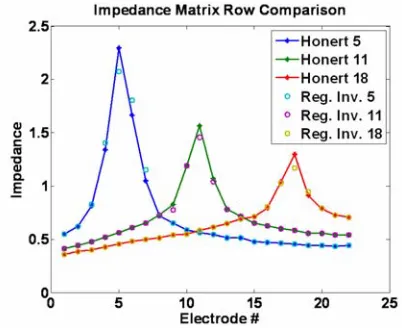
Results using both of these regularization terms and the data provided by Hornet are shown in Figure 1. Not surprisingly the results away from the diagonal terms compare well with Hornet and Kelsall. They differ near the diagonal because the average linear projection used here is different from the maximum linear projection used by Hornet and Kelsall.
[image:9.612.93.294.296.460.2]The above solution does not extend what Hornet and Kelsall have done in a very useful manner and in fact it may be worse in some ways. However it does offer the possibility to improve things in the future. For example this approach needs no adaptation to accommodate multiple data sets for an over-determined solution. Also, a third regularization term could be added that forces the impedance matrix solution toward a symmetric result. Furthermore, a regularization term could be used to extrapolate beyond the end of the array to create virtual electrodes. These could then be used to reduce auditory excitation beyond the end of the cochlear array.
Figure 1 Comparison of regularized inversion impedance matrix calculation with original data.
4. S OLV IN G TH E P H AS ED AR RAY IN V ERS ION WIT H R E GU L AR IZ E D IN VERS ION
A more immediate benefit can be seen when regularized inversion is used to perform the impedance matrix inversion of Equation 2. In this case we do not possess any a priori estimate of the solution itself. However the solution can be influenced in a desirable manner. Three examples of desirable solution influence are demonstrated here including:
1. Minimize the “effort” or rms current required for focused excitation.
2. Minimize the total current across all electrodes and thus reduce the “penalty current” referred to by Honert and Kelsall.
3. Minimize the “tails” (those electrodes away from the focus point) of the excitation current distribution.
Simulations were conducted by assuming that the impedance matrix supplied by Honert and Kelsall for subject 1 is exact. A noisy impedance matrix was created by adding normally distributed noise with zero mean and standard deviation of 0.01. This standard deviation is slightly larger than that estimated by Honert and Kelsall. A noisy matrix was then used to calculate the currents required to produce a focused voltage excitation at electrode 7. In subsequent plots showing minimized variables versus rms voltage error each data point is the average of 100 simulations with independent noisy impedance matrices.
MINIMIZING THE CURRENT EFFORT
The rms current can be minimized (along with the solution rms error) by using a single regularization term in Eq. 5; setting the weighting matrix, H1, to the identity matrix; and setting the
estimate vector, x, to zeros. In this manner the sum of the squares of the individual currents will be minimized along with the rms solution error. The inverse of the impedance matrix was calculated in this manner for µ1 ranging between 0 and 1000. The objective was to induce a voltage at electrode 7
only. The resulting rms current is plotted against the voltage error in Figure 2. As the Lagrange multiplier, µ1, is increased the rms current decreases but at the expense of increasing error. This
curve is relatively linear suggesting that it may not be advantageous to use this approach. A specific solution of this type is shown in Figure 3. As one would expect, minimizing the rms current forces all node currents toward zero.
[image:10.612.316.534.428.588.2]ˆ
[image:10.612.93.300.432.592.2]Figure 2 rms Current versus rms voltage error when the rms current is minimized using regularized inversion.
Figure 3 Array currents and induced voltages. Location of this solution in Fig. 2 indicated by red star.
MINIMIZING THE NET CURRENT
A second way in which regularized inversion may favourably affect the solution is to minimize the net current flowing into the tissue. This will minimize the “penalty current” described by Honert
and Kelsall. The net current can be minimized by using a single regularization term and populating the weighting matrix, H1, with ones and populating with zeros. This will force the sum of all currents towards zero. In this manner, the larger we make µ1 the smaller the net current will be.
Results from these simulations are shown in Fig. 4 which shows the total current versus rms voltage error as µ1 varies between 0 and 1e6. As demonstrated, if one can accept about twice the voltage
[image:11.612.93.291.238.400.2]error, the total current can be decreased several orders of magnitude. The region which the data in Figure 4 occupies in Figure 2 is indicated in Figure 2 by the red oval. Recall that the data points in Fig 4 are the averages for 100 separate trials. The standard deviation of the rms voltage error is rather large (about 2e-4) for larger values of µ1 (the right portion of the graph). A specific trial from
these simulations is shown in Figure 5. Note that minimizing the total current results in alternating positive/negative current values. However, the individual current values are not pushed toward zero as occurred in the previous case.
1
ˆ
x
[image:11.612.316.528.238.398.2]Figure 4 Total Current versus rms voltage error when the total current is minimized using regularized inversion.
Figure 5 Array currents and induced voltages. Location of this solution in Fig. 4 indicated by a black star.
MINIMIZING THE CURRENT “TAIL”
Finally, it may be desirable for the current to tend toward zero away from the target electrode. This can be accomplished by forcing the solution to be smooth except near the target electrode. A smooth solution is encouraged by setting H1 equal to
⎥
⎥
⎥
⎥
⎥
⎥
⎥
⎥
⎥
⎥
⎥
⎦
⎤
⎢
⎢
⎢
⎢
⎢
⎢
⎢
⎢
⎢
⎢
⎢
⎣
⎡
−
−
−
−
−
=
O M M M M M M M L L L L L L L2
1
0
0
0
0
0
0
2
1
0
0
0
0
0
0
0
0
0
0
0
0
0
0
0
0
0
0
0
0
0
0
0
0
0
0
0
0
0
1
2
1
0
0
0
0
0
1
2
2H
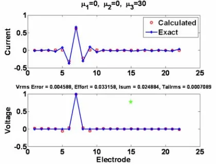
(9) [image:11.612.149.355.534.686.2]Eq. 9 defines a tri-diagonal matrix, with 2 on the main diagonal and -1 on the first off-diagonals. Furthermore the rows of the targeted electrode, plus the row above and below, are set to zero. The effect of setting a row to {-1 2 -1} is to approximate the second derivative of the solution. Therefore the curvature of the solution is minimized. The effect of the zeroed rows is to allow the solution to be un-smooth near the target electrode. Results from simulations are shown in Figure 6 which shows
[image:12.612.317.527.146.311.2]Figure 6 rms Current versus rms voltage error when the current tail is minimized using regularized inversion. This data occupies the grey box in Figure 2.
Figure 7 rms Current “tail” versus rms voltage error.
the rms current versus the rms voltage error for 0< µ1<1e4 . Overall the rms current is
changed very little. This is because the rms current is dominated by the targeted electrode and two neighbouring electrode currents. Since the weighting matrix is zero for these electrodes there is no effect on their values. Note that Fig. 6 occupies the grey box region of Fig. 2. Away from the targeted electrode there is a significant effect on the current. This is demonstrated in Figure 7 which shows the rms tail current versus the rms voltage error for 0< µ1<1e4. The rms tail current is
the rms of all currents except the targeted electrode and the two neighbouring electrodes. As shown in Figure 7 the tail rms can be significantly reduced. Figure 8 shows a specific solution for current tail weighing which is located on Figures 6 and 7 by the green star. As can be seen, all of the currents in the tails are forced toward zero while the central currents are not. Figure 5 Array currents and induced voltages. Location of this
solution in Fig. 4 indicated by a green star.
[image:12.612.91.301.396.558.2]5. S OLV IN G TH E INVERSIO N WITH S IN GULAR VALUE DECO MPOS TION
Another method of quantifying and rectifying problems with poorly conditioned matrices is with Singular Value Decomposition. Applying SVD to the impedance matrix of Equation 1 results in
T
W UΛ
Z= (10)
where U and W consist of columns of orthonormal vectors and Λ is a diagonal matrix of singular values. Making use of Equation (3) the solution to Equation 1 can be written as
∑
=
−
=
=
Mi 1 i
1
v
u
w
v
U
W
Λ
i
Ti i T
1
λ
(11)If any of the singular values, λi, are small compared to the largest then the matrix is ill
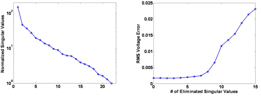
[image:13.612.96.520.364.521.2]conditioned. The result in the solution is that small singular values can have a large influence on the solution. A common method is to set the inverse of small singular values (those less than 1% of the maximum for example) equal to zero. This was applied to the data supplied by Honert and Kelsall and the results are shown in Figure 8. It seems that although the matrix is poorly conditioned (conditioning number of 136) the elimination of small singular values does not result in a more accurate solution.
Figure 7 Normalized singular values for Honert and Kelsall subject 1 impedance matrix.
Figure 8 RMS voltage error versus the number of eliminated singular values.
6. C ONC L US IO NS
Overall these results show that it may be possible to improve on the approach of Honert and Kelsall through the use of regularized inversion. Assuming that decreasing net current and decreasing current “tails” are beneficial result, then this approach offers substantial benefit. More importantly these results show that regularized inversion can be used to significantly alter the solution in desirable ways. Future work should focus on specifying what constitutes a “desirable” solution and developing methods for expressing this in regularization terms.