Efficient Image Haze Removal using Aging Particle Swarm Optimization based Dark Channel Prior

Volume 8, No. 5, May – June 2017

International Journal of Advanced Research in Computer Science RESEARCH PAPER

Available Online at www.ijarcs.info

Efficient Image Haze Removal using Aging Particle Swarm Optimization based Dark

Channel Prior

Jaswinder Kaur

Department of Computer Engineering and Technology Guru Nanak Dev University

Amritsar, India

Prabhpreet Kaur

Department of Computer Engineering and Technology Guru Nanak Dev University

Amritsar, India

Abstract: Haze reduces the visibility of a scene. Haze removal is one of the challenging tasks as it depends upon the unknown depth information. This paper presents an efficient method to remove haze from a single image based on the aging particle swarm optimization and dark channel prior. In the proposed method firstly, thickness of the haze is evaluated using dark channel prior, then aging particle swarm optimization is used to monitor and locate the best optimized value for restoration. The adaptive histogram equalization is applied to increase the contrast of the degraded image. An enhanced and optimized image is obtained. Some standard parameters such as mean square error, peak signal to noise ratio and bit error rate are utilized to compare the existing and proposed method. This method is useful for many computer vision and image understanding applications. The experimental results demonstrate that the proposed approach provides higher quality results.

Keywords: haze, dark channel prior, aging particle swarm optimization, airlight, adaptive histogram equalization.

I. INTRODUCTION

The quality of outdoor images is usually degraded [1], because the light getting absorbed or dispersed from the atmospheric particles in the existence of fog, haze or smoke. The degraded images lose contrast and color fidelity [2]. Hence, the visibility of the scene is reduced. Many automatic systems have failed to work, which highly depend to the input images. Therefore, enhancing the entire process of image dehazing will benefit several computer vision and image understanding applications [3] like image classification [4-6], aerial imagery [7], video/image retrieval [8-10], object detection and remote sensing [11]-[12], video analysis and recognition [13-15]. However, haze eliminating is one of the difficult tasks as it depends upon the unknown depth information [16].

Earlier analysts used the traditional methods to eliminate the haze from a single image, i.e. dehazing techniques based on histogram [17]-[18]. Since, a single image could not provide more information. Eventually, analysts made an effort to enhance the dehazing results using multiple images. Schechner et al. [19]-[20], proposed polarization based methods, where several images were taken with various levels of polarization. Narasimhan et al. [21]-[22] proposed dehaze method with many images under the similar atmospheric conditions.

Later, major improvement had been made by using the physical model. Tan [23] introduced an automatic method that just needed a single input image. The image contrast was maximized according to Markov Random Field (MRF). Even though Tan’s method obtained better results. However, the disadvantage was that it tends to generate oversaturated pictures. Fattal [24] proposed Independent Component Analysis (ICA) to remove haze from the color images. But, this method took more time as well as not applicable for grayscale images. Chavez [25] motivated from the dark object subtraction method, He et al. [26] proposed an easy method, and a successful picture of the Dark Channel Prior (DCP) to eliminate the haze out of the picture and restored dehaze image using an atmospheric scattering model. This method needed the soft mating to refine transmission map,

[image:2.595.37.280.53.242.2]

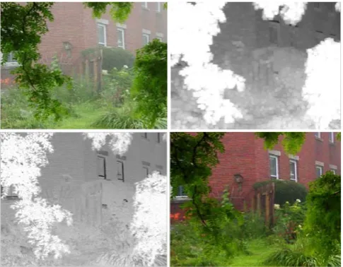
Figure 1. An overview of proposed dehazing approach. Top-left: original hazy image. Top-right: dark channel prior. Bottom-left: Transmission

filtered map. Bottom-right: picture without haze.

This paper presents the following. Part 2, presents an overview of the dark channel prior which is related to our propose work. Part 3, explains the proposed haze removal techniques. Part 4, represents the Methodology flowchart. Part 5, presents the qualitative and quantitative experimental results. Finally, part 6, presents the conclusion and future work.

II. BACKGROUND

The dark channel prior and optical model of hazy images is closely related to our proposed work [1], [26], [36].

A. Optical model of hazy image

The below formula defines the occurrence of the hazy images:

( ) ( ) ( )

u

j

u

t

u

A

(

t

( )

u

)

I

=

+

1

−

(1)

where

I

is the original hazy picture,

u

is the pixel index,

j

is an image without haze, the transmission map is

t

, indicates the portion of light which is not dispersed, and

A

is generally the atmospheric light. The initial expression

( ) ( )

u

t

u

j

is known as direct attention and the second

expression is known as

A

(

1

−

t

( )

u

)

airtight.

B. Dark channel prior

The dark channel prior approach depends on the observation, in which a few pixels possess very low intensity within a minimum of one color channel. The main process of image dehazing is to approximate the transmission map

t

and atmospheric light

A

from hazy picture. To estimate both the atmospheric light

A

and transmission

t

, He K. et al. initially proposed the dark channel prior method. The dark channel

j

dchannel for a random image

j

is shown as:

( )

( ) (

) ( )













Ω

=

j

v

b

g

r

c

u

v

u

j

dchannel c

2

,

2

,

2

min

min

ε

ε

(2)

where

j

cdefines the r2 (red), g2 (green), b2 (blue) color

channel of the original picture

j

and

Ω

( )

u

is the regional patch origin at u. Two minimum operators are:

( 2, 2, 2)

min

_{cε r b g} is the minimum operator to examine the

minimum value in the three color channels and

min

_{vεΩ( )u} is the minimum filter.

C. Transmission Estimation

If

j

is a dehazed picture, excluding sky regions, then the dark channel associated with

j

is commonly approached to zero:

0

→

dchannel

j

(3) Haze image equation (1) is normalized by

A

to estimate the

atmospheric light.

( ) ( ) ( )

t

( )

u

A

u

j

u

t

A

u

I

c c c c

−

+

=

1

(4)

we suppose that the transmission map within a regional patch

( )

u

Ω

is actually constant. Then, this transmission is represented as

t

2

( )

u

. Hence, the dark channel can be computed from both sides of the equation (4). Put two minimum operators on both sides:

( )

( )

( ) ( )

( )

t

( )

u

A

v

j

c

u

v

u

t

A

v

I

c

u

v

c c c c

2

1

min

min

2

min

min

−

+













Ω

=













Ω

ε

ε

(5)

The dehaze image is

j

, whose dark channel is always tending to zero, due to dark channel prior:

( )

min

( )

min

( )



=

0











Ω

=

j

v

c

u

v

u

j

dchannel c

ε

(6)

Since

A

cis being often positive, and tends to:

( )

min

( )

0

min

=













Ω

c c

A

v

j

c

u

v

ε

(7)

Putting (7) into (5), multiplicative terms can be removed and transmission

t

2

can be approximated as shown:

( )

( )













Ω

−

=

c _c

A

v

I

c

u

v

z

u

t

min

)

(

min

1

2

ε

(8)

where z is a constant value in order to maintain a tiny amount of haze (0<z<1). The transmission map is directly provided by this equation.

D. Restoration of Input Image

Finally, the picture is restored using below equation:

( )

(

t

u

t

)

A

u

I

u

j

=

+

0

,

max

)

(

)

(

(9)

0

[image:3.595.83.228.55.271.2]

Figure 2. Flow diagram of dark channel prior [1]

III. PROPOSED TECHNIQUES

The proposed method is Aging Particle Swarm optimization using dark channel prior and adaptive histogram equalization is applied to enhance the picture contrast. The flow diagram of the proposed method is shown in Fig. 5. The detail of each process is explained in the below sub-sections.

A. Adaptive histogram equalization

The Adaptive histogram equalization (AHE) process is an advancement in the existing histogram equalization technique. The AHE has been often used to get better contrast images. It improves the inequality associated with pictures through modifying the values within the intensity image. In comparison to histogram equalization, it is implemented on very small data regions (tiles) instead of the whole image [37], [38].

B. Proposed algorithm

The Aging particle swarm optimization is a population dependent search method, influenced by the social interaction of the bird flocks. The age (Ɵ) and the lifespan (Φ) of the gbest particle are adaptively altered with respect to its leading power. Whenever the lifespan of the gbest is exhausted, then it is exchanged by newly developed particles. [39], [40], [41].

The operation of Aging Particle Swarm Optimization is shown as:

• Initialization: Initialize all the particles developed in the search space, velocities initialized to 0. The best particle in the search space is selected as the gbest. The lifespan and the age of the gbest particle is set in order Φ=Φ0

• Updating Velocity: Every particle velocity is updated according to the given equation:

and Ɵ=0 respectively.

(

j j

)

(

j j

)

j

j

w

c

r

pbest

p

c

r

gbest

p

v

=

₋₁

+

₁₁

∗

₁₁

∗

−

+

₂₂

∗

₂₂

∗

−

(10)

where vj and pj are current velocity and position of particles and vj-1 is previous velocity of the jth particle. The pbestj and gbestj

11

r

are the position of a j particle having best value found so far, within the

entire population; the convergence behavior of the aging PSO is controlled by w; and

r

₂₂ are arbitrary parameters vary from [0, 1];

c

₁₁and

c

₂₂ manage how long a particle proceeds in a single iteration.

• Position Updating: The position of the entire particles updated with the successive iteration in the unit time interval is as:

j j

j

p

v

p

=

₋1

+

(11)

• Updating pbest and gbest: When the position of the newly generated particle pj is better than the pbestj, then it becomes the new pbestj. If in this iteration the best position is generated, then the gbestj can be updated to the newly best position. Here the gbestj

( ) (

j j

)

j

j

p

if

p

pbest

pbest

=

>

represents the best solution.

( ) (

j j

)

j

j

g

if

g

gbest

gbest

=

>

• Lifespan control: Immediately after updating the position of all particles, the leading power of the gbest increase the performance of the entire swarm. The lifespan (Φ) is modified through a lifespan controller and the age (Ɵ) is increased by 1. When Ɵ> Φ i.e. lifespan is exhausted, then move to step 6. Otherwise, move to step 8.

• Creating a challenger: To challenge the gbest, a new particle is created by the challenger.

• Evaluate the challenger: If a newly created challenger possesses more leading power, then it becomes the new gbest by replacing the old gbest. The lifespan and the age of the new gbest are initialized to Φ= Φ0

• Termination Checking: When the number of

iterations (FE) is greater than the maximum predefined iteration (maxi-evaluation), then the algorithm terminates. Otherwise the new iteration starts from step 2.

and Ɵ=0 respectively.

The proposed aging particle swarm optimization algorithm mainly performs three tasks.

• Firstly the lifespan of the gbest is adjusted by the lifespan controller based on its leading power. • Secondly, a new particle is created to challenge the

old gbest particle.

• Finally a qualifying criterion is used to determine whether the created particle is accepted as a new gbest

• Lifespan controller: The main function of lifespan controller is to control the leading power of the gbest. If the gbest has best leading power, then the controller increases its lifespan, otherwise, reduces its lifespan.

Input Hazy image I(u)

Calculate dark channel

Atmospheric light (A) is estimated

Estimating the transmission map

[image:4.595.93.511.57.568.2]

Figure 3. Flow diagram of proposed aging particle swarm optimization algorithm [40]

IV. PROPOSED METHODOLOGY

Fig. 5 shows the methodology of the proposed method. The haze is not removed by existing methods efficiently. Therefore, we propose the new techniques which consist of the dark channel prior, adaptive histogram equalization and aging PSO. The working of the proposed method is defined as:

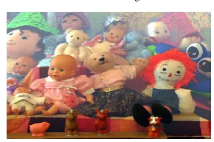
• Firstly, hazy image is passed to the system shown in fig. 4.

Figure 4. Original hazy image.

Velocity and position are initialized

Update pbest and gbest Ɵ = 0

Ф = Ф0

All the particle velocity and position are updated based on (10) and (11)

Lifespan adjust Ф Ɵ= Ɵ +1

End Ɵ> Ф

No

Start

FE<maxi_ev alation

Best solution has been found by the algorithm

Yes

Create a new challenger

Accept the Challenger as a

new gbest

Yes _No

Set the challenger as a new gbest

The Swarm status is rolled back

Ɵ =0 Φ = Φ0

Ɵ=Φ-1

Yes

No

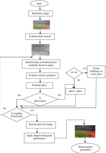
[image:4.595.344.524.622.724.2]

[image:5.595.68.500.90.709.2]

Figure 5. Flow diagram of proposed haze removal methodology.

Start

Read hazy image

Evaluate dark channel

Initialize haze restoration factor randomly based on aging

Evaluate velocity and pbest

Is pbest<gbest

gbest = pbest

Apply adaptive histogram equalization Is stopping

Criteria met

Restore haze free image

Return quality parameters yes

No yes

Evaluate pbest

No

Ɵ> Ф

No

yes Create

[image:6.595.53.258.71.219.2]

• The thickness of haze is computed by applying dark channel prior to the hazy image.

Figure 6. Dark channel prior of hazy image

• Initialize the haze restoration factor randomly based on aging.

• The position and velocity of every particle are evaluated and compare with the best particle.

• If the position of the newly generated particle is better than, pbestj then it becomes new gbestj

• The dehaze image is restored using restored equation (9).

.

• Finally, the adaptive histogram equalization is applied to increase the contrast of the images.

Figure 7. Haze free image.

• The quality parameters are returned.

• If the lifespan of the gbest particle is exhausted, then the challenger creates a new particle, which is being accepted as a new gbest, and step from 6 to 8 are repeated.

• If the number of iterations is low, than the chosen, then steps from 4 to 8 are repeated.

V. EXPERIMENTAL RESULTS

The proposed algorithm is designed and executed in the MATLAB R2013a environment utilizing an image processing toolbox on a i5-2.50GHz PC with 8 GB RAM. To show the effectiveness of the proposed method, it has been tested on many benchmark images as well as qualitatively compare with He et al.’s [26], Nishino et al. [34], and Guo et al. [35] method

The dataset is collected from:

http://www.cs.huji.ac.il/~raananf/projects/dehaze_cl/results/. http://perso.lcpc.fr/tarel.jean-philippe/.

Many (3000) road hazy images are collected from FRIDA dataset.

A. Qualitative comparison of hazy images

Good results are given by all the dehazing algorithms, but it is very complicated to rate them visually. In order to compare them various benchmark images are taken, which consist of large gray and white region, because some existing methods are unable to detect white regions.

Fig. 8 indicates the qualitative evaluation along with the existing three state-of-the-art dehazing methods [26], [34], [35] on benchmark hazy images. Fig. 8 (a) shows original hazy pictures Fig. 8 (b-d) depicts final results of He et al. [26], Nishino et al. [34], and Guo et al. [35], respectively. The proposed algorithm results are given in Fig. 8 (e). Almost all the haze is eliminated from Nishano’s final results, and also objects are well restored. But it suffers from over enhancement. It has been shown in Fig. 8 (c) the restored pictures are suffering from distortion and over saturation; particularly in the fifth picture of the swan (shade of the swan is usually modified to dark). On the other hand, the final results of He et al. is looking good (shows Fig. 8 (b)). There are no halo artifacts and the thick haze within the distance is well eliminated. But in the white object regions color distortion still appeared. This algorithm cannot handle the sky regions (shown in Fig. 8 (b) sixth image of the mountain) and also tends to overestimate the particular transmission.

[image:6.595.65.276.362.502.2]

[image:7.595.50.546.67.747.2]

(a) (b) (c) (d) (e)

B. Quantitative comparison of hazy images

Fig. 9 shows a quantitative comparison of the existing Guo et al. [35] and proposed algorithm. Fig. 9 (a) presents the hazy picture. Fig. 9 (b) shows the Guo et al. results [35] and Fig. 9 (c) indicates the final results of the proposed algorithm. To further prove the overall performance of the aging particle swarm optimization and its advantage over the existing approach, the quantitative evaluation is also conducted on hazy images depicts in Fig. 9.

[image:8.595.36.289.180.709.2]

(a) (b) (c) Figure 9. Shows quantitative comparison of various images. (a) hazy picture to

be dehazed (b) Guo et al [35] approach (c) proposed approachThe proposed method is examined based on some parameters, i.e. Peak Signal to Noise Ratio (PSNR), Mean Square Error (MSE) and Bit Error Rate (BER). The final results

demonstrate that the proposed approach is superior to existing one.

• Mean Square Error: For better result mean square error must be reduced. The mean square error provides the cumulative error for the original hazy image and output image. The less MSE, results in a minimum error. The mean square error is measured as [42]:

(

)

(

)

(

)

2

,

,

,

n

M

m

n

N

m

n

m

MSE

=

Σ

_in

−

_op (12) where, m and n are the number of rows and columns of

the input picture respectively. Min is the input image and Nop is the output image.

• Peak signal to noise ratio: The peak signal to noise ratio provides the quality measurement of the original input image and restored enhance image. The greater value of PSNR shows a better quality image. The PSNR can be computed using the below equation. [42]:













=

MSE

R

PSNR

10

log

₁₀ (13)

where R is maximum fluctuation in the original input image.

• Bit error rate: The bit error rate must be minimized for better result. The less value of BER shows a better quality image. It is defined as [42]:

send

bits

of

Number

errors

of

Number

BER

=

(14)

It can be measured as:

PSNR

BER

=

1

(15) [image:8.595.311.563.452.590.2]

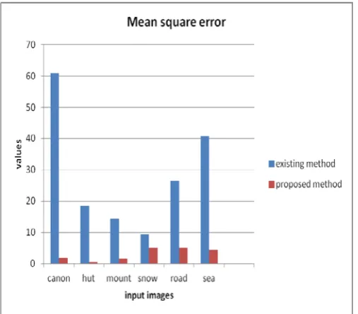
Table I. Evaluation of Mean Square Error

Image name Image

resolution

Existing method [35]

Proposed method

canon 600×525 0.6093 0.0186 hut 600×450 0.1858 0.0063

mount 512×384 0.1434 0.0161

snow 876×584 0.0936 0.0507

road 640 ×480 0.2642 0.0506

[image:8.595.314.564.623.757.2]

sea 1600×928 0.4070 0.0429

Table II. Evaluation of Peak signal to noise ratio

Image name Image resolution

Existing method [35]

Proposed method

canon 600×525 50.2821 65.4433

Hut 600×450 55.4403 70.1090

mount 512×384 56.5656 66.0551

Snow 876×584 58.4180 61.0821

Road 640 ×480 53.9115 61.0923

sea 1600×928 52.0349 61.8101

Image name

Image resolution

Existing method [35]

Proposed method

canon 600×525 0.0199 0.0153

Hut 600×450 0.0180 0.0143

mount 512×384 0.0177 0.0151

snow 876×584 0.0171 0.0164

road 640 ×480 0.0185 0.0164

sea 1600×928 0.0192 0.0162

[image:9.595.312.559.55.280.2]

Table 1, Table 2 and Table 3 compares the MSE, PSNR and BER of Existing [35] and proposed method. The proposed method shows better quantitative results.

[image:9.595.36.290.250.472.2]

Figure 10. Mean Square error of existing and proposed method.

Figure 11. Peak signal to noise ratio of existing and proposed method.

Figure 12. Bit error rate of existing and proposed method.

Fig. 10, Fig. 11 and Fig. 12 indicates a comparative evaluation with the MSE (mean square error) PSNR and BER associated with an existing approach (blue color) and Proposed Approach (red color) of various images. The Graph shows decrease in MSE, BER and increase in PSNR value for every image utilizing the proposed method. This presents a vast improvement within image quality.

VI. CONCLUSION

A new, single image dehazing technique is presented that maximize the visibility of the hazy image. The proposed methodology integrates dark channel prior and aging particle swarm optimization. The proposed algorithm tries to find the best solution in the entire search space. The contrast of the hazy images is enhanced using Adaptive histogram equalization. The Aging PSO removes the limitations of the existing methods. The proposed method is tested on various benchmark hazy images. The experimental results demonstrate that the proposed approach provides higher quality dehaze images. The quantitative measurements like PSNR, MSE and also BER verifying the efficiency of the proposed method over the existing Genetic algorithm. The new method is applicable in many computer vision and image understanding applications. We would like to extend our work to remote sensing hazy images.

VII. REFERENCES

[1] Y. Xu, X. Guo, H. Wang, F. Zhao, L. Peng, “Single Image Haze Removal Using Light and Dark Channel Prior,” Communications in China (ICCC), 2016 IEEE/CIC International Conference on, 2016. doi: 10.1109/ICCChina.2016.7636813

[2] Q. Zhu, S. Yang, P. A. Heng, X. Li, “An Adaptive and Effective Single Image Dehazing Algorithm Based on Dark Channel Prior,” Robotics and Biomimetics (ROBIO), 2013 IEEE International Conference on, 2013, pp. 1796-1800. doi: 10.1109/ROBIO.2013.6739728

[3] Q. Zhu, J. Mai, L. Shao, “A Fast Single Image Haze Removal Algorithm Using Color Attenuation Prior,” IEEE Transactions on Image Processing, vol. 24, no. 11, pp. 3522-3533, November 2015. doi: 10.1109/TIP.2015.2446191

[image:9.595.36.288.520.741.2]

25, no. 7, pp. 1359-1371, July 2014. doi: 10.1109/TNNLS.2013.2293418.

[5] Y. Luo, T. Liu, D. Tao, C, Xu, “Decomposition-Based Transfer Distance Metric Learning for Image Classification,” IEEE Transactions on Image Processing, vol. 23, no. 9, Sept. 2014. doi: 10.1109/TIP.2014.2332398

[6] D. Tao, X. Li, X. Wu, “Maybank S J. Geometric Mean for Subspace Selection,” IEEE Transactions on Pattern Analysis and Machine Intelligence, vol. 31, no. 2, pp. 260-274, Feb 2009. doi: 10.1109/TPAMI.2008.70

[7] G. A. Woodell, D. J. Jobson, Z-U Rahman, G. Hines, “Advanced image processing of aerial imagery. Proc SPIE,” vol. 6246, pp. 62460E, May 2006. doi:10.1117/12.666767.

[8] J. Han, X. Ji, X. Hu, et al. “Representing and retrieving video shots in human-centric brain imaging space,” IEEE Transactions on Image Processing, vol. 22. no. 7, pp. 2723-2736, July 2013. doi:10.1109/TIP.2013.2256919.

[9] J. Han, K. Ngan, M. Li, H. J. Zhang, “A memory learning framework for effective image retrieval,” IEEE Transactions on Image Processing, vol. 14, no. 4, pp. 511–524, April. 2005. doi: 10.1109/TIP.2004.841205

[10] D. Tao, X. Tang, X. Li, X. Wu, “Asymmetric Bagging and Random Subspace for Support Vector Machines-Based Relevance Feedback in Image Retrieval,” IEEE Transactions on Pattern Analysis and Machine Intelligence, vol. 28, no. 7, pp. 1088-1099, July 2006. doi:10.1109/TPAMI.2006.134.

[11] J. Han, D. Zhang, G. Cheng, L. Guo, J. Ren, “Object detection in optical remote sensing images based on weakly supervised learning and high-level feature learning,” IEEE Transactions on Geoscience and Remote Sensing, vol. 53, no. 6, pp. 3325-3337, June 2015. doi:10.1109/TGRS.2014.2374218.

[12] J. Han, P. Zhou, D. Zhang, et al. “Efficient simultaneous detection of multi-class geospatial targets based on visual saliency modeling and discriminative learning of sparse coding,” ISPRS J Photogramm Remote Sensing,. vol. 89, pp. 37-48, March 2014. doi:10.1016/j.isprsjprs.2013.12.011.

[13] L. Liu, L. Shao, “Learning Discriminative Representations from RGB-D Video Data,” In Proceedings of the Twenty-Third international joint conference on Artificial Intelligence, Beijing, China, 2013, pp. 1493–1500

[14] D. Tao, X. Li X, X. Wu, S. J. Maybank, “General Tensor Discriminant Analysis and Gabor Features for Gait Recognition,” IEEE Transactions on Pattern Analysis and Machine Intelligence, vol. 29, no. 10, pp. 1700-1715. doi: 10.1109/TPAMI.2007.1096

[15] Z. Zhang, D. Tao, “Slow Feature Analysis for Human Action Recognition,” IEEE Transactions on Pattern Analysis and Machine Intelligence, vol. 34, no. 3, pp. 436-450, March 2012. doi:10.1109/TPAMI.2011.157.

[16] Y. K. Wang, C. T. Fan, “Single Image Defogging by Multiscale Depth Fusion,” IEEE Transactions on image processing, vol. 23, no. 11, pp. 4826 - 4837, November 2014. doi: 10.1109/TIP.2014.2358076

[17] T. K. Kim, J. K. Paik, B. S. Kang, “Contrast enhancement system using spatially adaptive histogram equalization with temporal filtering,” IEEE Transactions on Consumer Electronics, vol. 4, no. 1, pp. 82-87, Feburary 1998. doi: 10.1109/30.663733

[18] J. Y. Kim, L. S. Kim, S. H. Hwang, “An advanced contrast enhancement using partially overlapped sub-block histogram equalization,” IEEE Transactions on Circuits and Systems for Video Technology, vol. 11, no. 4, pp. 475-484, April 2001. doi: 10.1109/76.915354

[19] Y. Y. Schechner, S. G. Narasimhan, S. K. Nayar, “Instant dehazing of images using polarization,” in Proceedings of the IEEE Computer Society Conference Computer Vision and Pattern Recognition(CVPR), 2001, pp. 325-332. doi: 10.1109/CVPR.2001.990493

[20] Y. Y. Schechne, S. G. Narasimhan, S. K. Nayar, “Polarization-based vision through haze. Applied Optics,” vol. 42, no. 3, pp. 511-525, 2003. doi: 10.1364/AO.42.000511

[21] S. G. Narasimhan, S. K. Nayar, “Contrast restoration of weather degraded images,” IEEE Transactions on Pattern Analysis and Machine Intelligence, vol. 25, no. 6, pp. 713–724, June 2003. doi: 10.1109/TPAMI.2003.1201821

[22] S. G. Narasimhan, S. K. Nayar, “Interactive (de) weathering of an image using physical models,” in Proceedings IEEE Workshop color Photometric Methods Computer Vision, vol. 6, pp. 1, 2003.

[23] R.T. Tan, “Visibility in Bad Weather from a Single Image,” IEEE Conference on Computer Vision and Pattern Recognition, 2008, pp. 1-8. doi: 10.1109/CVPR.2008.4587643

[24] Fattal R, “Single Image Dehazing,” ACM Transaction Graph, vol. 27, no. 3, pp. 72, August 2008. doi: 10.1145/1399504.1360671

[25] P. S. JR. Chavez, “An improved dark-object subtraction technique for atmospheric scattering correction of multispectral data,” Remote Sensing of Environment, vol. 24, no. 3, pp. 459-479, April 1998. doi: 10.1016/0034-4257(88)90019-3

[26] K. He, J. Sun, X. Tang, “Single Image Haze Removal Using Dark Channel Prior,” IEEE Transactions on Pattern Analysis and Machine Intelligence, vol. 33, no. 12, pp. 2341 - 2353, December 2011, doi: 10.1109/TPAMI.2010.168

[27] J. P. Tarel, N. Hautiere, “Fast Visibility Restoration from a Single Color or Gray Level Image,” IEEE International Conference on Computer Vision, 2009, pp. 2201-2208 doi: 10.1109/ICCV.2009.5459251

[28] J. M. Liu, Y. G. Hao, Y. B. Zhu, “An Single Image Dehazing Algorithm Using Sky Detection and Segmentation,” 7th International Congress on Image and Signal Processing, 2014, pp. 248-252. doi :10.1109/CISP.2014.7003786

[29] K. B. Gibson, D. T. Vo, T. Q. Nguyen, “An investigation of dehazing effect on image and video coding,” IEEE Transactions on Image Processing, vol. 12, no. 2, pp. 662-673, Feburary 2012. doi: 10.1109/TIP.2011.2166968

[30] J. Yu, C. Xiao, D. Li, “Physics-based fast single image fog removal,” in Proc. IEEE 10th International Conference Signal Process. (ICSP), Oct. 2010, pp. 1048–1052. doi: 10.1109/ICOSP.2010.5655901

[31] K. He, J. Sun, X. Tang, “Guided image filtering,” IEEE Transactions on Pattern Analysis and Machine Intelligence , vol. 35, no. 6, pp. 1397-1409, June 2013. doi: 10.1109/TPAMI.2012.213

[32] A. Levin, D. Lischinski, Y. Weiss, “A closed-form solution to natural image matting,” IEEE Transaction on Pattern Analysis and Machine Intelligence., vol. 30, no. 2, pp. 228–242, Feburary 2008. doi:10.1109/TPAMI.2007.1177

[33] W. Bo, Z. Zhihui, Z. Zhiqiang, S. Kang, “Fast Single Image Dehazing Using Iterative Bilateral Filter,” 2nd international conference in information engineering and computer science (ICIECS), 2010. doi: 10.1109/ICIECS.2010.5678374

[34] K. Nishino, L. Kratz, S. Lombardi, “Bayesian Defogging,” International Journal of Computer Vision, vol. 98, no. 3, pp. 263–278, July 2012. doi: 10.1007/s11263-011-0508-1

[35] F. Guo, H. Peng, J. Tang, “Genetic algorithm-based parameter selection approach to single image defogging,” Information Processing Letters, vol. 116, no. 10, pp. 595-602, October 2016. doi: 10.1016/j.ipl.2016.04.013

[36] B. Li, S. Wang, J. Zheng, L. Zheng, “Single image haze removal using content-adaptive dark channel and post enhancement,” IET Computer Vision, vol. 8, no. 2, pp. 131-140, April 2014. doi: 10.1049/iet-cvi.2013.0011

Electronics, and Optimization Techniques (ICEEOT), 2016, pp. 4074-4078. doi: 10.1109/ICEEOT.2016.7755480

[38] Z. Xu, X. Liu, N. Ji, “Fog removal from color images using contrast limited adaptive histogram equalization,” 2nd International Conference on Image and Signal Processing, 2009, doi: 10.1109/CISP.2009.5301485

[39] A. Kaur, M. D. Singh, “An Overview of PSO- Based Approaches in Image Segmentation,” International Journal of Engineering and Technology, vol. 2, no. 8, pp. 1349-1357, August 2012.

[40] W. N. Chen, J. Zhang, Y. Lin, N. Chen, Z. H. Zhan, H. S. H. Chung, Y. Li, Y. H. Shi, “Particle Swarm Optimization with an

Aging Leader and Challengers,” IEEE Transactions On Evolutionary Computation, vol. 17, no. 2, pp. 241-258, April 2013. doi: 10.1109/TEVC.2011.2173577

[41] P. P. V. G. D. Reddy, V. Vasavi, M. J. Stephen, “Fingerprint Image Enhancement through Particle Swarm Optimization,” International Journal of Computer Applications, vol. 66, no. 21, pp. 1-7, March 2013.