Gauge theories in three dimensions

Gauge Theories in Three Dimensions

by

Anthony Brian Waites, B.Sc.(Hons.)

A thesis submitted in fulfilment of the

requirements for the degree of

Doctor of Philosophy

- at the

University of Tasmania,

Hobart.

Declaration

Except as stated herein this thesis contains no material which has been accepted for the award of any other degree or diploma in any University. To the best of

my knowledge and belief, this thesis contains no material previously published or

written by another person, except where due reference is made in the text of the thesis.

Anthony B. Waites

5. Access to, and copying of. thesis

The thesis copy lodged in the University Library shall be made available by the University for consultation but, for a period of two years after the thesis is lodged, it shall not be made available for loan or photocopying without the written consent of the author and in accordance with the laws of copyright.

After a thesis has been examined. the following authority will apply. Please complete your request, and sign below.

(i) I agree/fB! M gr;e- that the thesis may be made available for loan.

(ii) I agree/"edmt-;J!fR!e""that the thesis may be made available for photocopying.

(iii) I note that my consent is required only to cover the two-year period following approval of my thesis for the award of my degree. After this, access to the Library copy will be subject only to any general restrictions laid down in Library regulations.

Signed~

.

1±)

•..•..

:.

~

'

Da~

r

I

/<

~

...

~

/:

..

.'

fi.I

.

Lodged in Morris Miller Central Library:.. . .. I.... . .... I 198.. . from which date the two years embargo will apply.

Acknowledgements

I wish to express my sincere thanks to my supervisor, Professor R. Delbourgo for his continual guidance and encouragement, and limitless patience throughout my time in Tasmania.

It is a pleasure to thank all the other past and present members of the theory group, including Dr. Peter Jarvis (for his sense of the ridiculous), Dr. Roland Warner, Dr. Ming Yung, Dr. Ian McArthur, -Dr. Dirk Kreimer, Dr. Dong-Sheng Liu (for giving us over 2000 years of anecdotes), Dr. Ioannis Tsohantjis, and Neville "Mr. Doom" Jones (for introducing an air of respectibility into the lives of the graduate students). All these people assisted me greatly in my work on this thesis, and more importantly filled me with warm memories of the place. Also, last but most, I'd like to thank Tim, who has become a truly great friend. Thanks Tim, for sharing your infinite dreams (infinity is hard to comprehend!); I'll see you in Antofagasta, mi amigo. Thanks also to THEO, without whom typesetting my thesis would have been impossible.

Mum and Dad, what can I say? Thanks for that night_ over 27 years ago, and for all the nights since. Thanks also to all my friends and flatmates both .here and in Melbourne, to Nit (my friend forever) and her family; to Petie (for being

specia0, Nettie, Matty, Helen, and the boBaggin man; to Anne, Martin, Oliver, ' Susan, and Jessie (for providing an escape from reality); to my brothers, Pete and Greg (for the years of love and torment) and their families, Nan, and Karie (for never forgetting me).

Abstract

Field theories in 2+ 1 space-time dimensions are of interest both intrinsically, due

to their novel properties such as actions which are topologically non-trivial, and

also due to their ability to explain of phenomena such as the fractional quantum

Hall effect and certain behaviour of high

Tc

superconductors, and for their use in

conformal field theory in 2D.

This thesis begins by considering scalar and spinor QED in 2+ 1 dimensions,

performing perturbation theory to study its behaviour (without allowing the

pres-ence or dynamical generation of a parity-violating photon mass). It is found, as

first noted by Jackiw and Templeton, that an IR instability prohibits such a

perturbative study. The gauge technique is adopted as a non-perturbative

alter-native, and the photon is allowed to be "dressed" in a cloud of fermion loops,

yielding results which encompass the perturbation results in the UV region, whilst

remaining finite at IR momenta.

Chern-Simons theory is then considered, where the photon is allowed to

ac-quire a parity-violating mass. In order to use dimensional regularization to handle

the. apparently UV divergent integrals which appear, a new formulation of the

theory is proposed, allowing the action to be written in arbitrary D dimensions,

I

'

so that the integrals can be safely evaluated. It is also found that the IR problems

which plague the conventional theory are no longer present, as the photon

prop-agator behaviour has been "softened" by the photon mass, allowing perturbation

results to be obtained.

Finally, the idea of mass generation within these theories is considered in more

detail, where we see that the presence of a fermion mass will cause a photon mass

to be dynamically generated, and vice versa. These ideas are then generalized for

Contents

-Declaration . . . . Acknowledgements Abstract . . . . Table of Contents . List of Figures . 1 Introduction

1.1 Field Theory in (2+1)D 1.2 The Gauge Technique . 1.3 Structure of the Thesis

2 Scalar Electrodynamics in (2+1)D 2.1 Background/Introduction

2.2 Perturbation Theory . 2.3 The Gauge Technique . 2.4 Gauge Covariance Relations 3 Spinor Electrodynamics in (2+1)D

3.1 Background . . . . . 3.2 Perturbation Theory. 3.3 The Gauge Tec~nique . 3.4 Gauge Covariance Relations 4 Chern-Simons Field Theory

4.1 Background . . . .

...

-

....

4.2 Dimensional Regularization 4.3 Perturbation Theory . . . .

5 Dynamical Mass Generation in Odd Dimensions

5.1 Mass Generation in (2+1)D . . . 5.2 QED in Higher Odd Dimensions .

6 Conclusion

6.1 Summary 6.2 Outlook

Appendices

Appendix A Appendix B Appendix C Appendix D

References

56

60

67

67

72 80

80

81 83

83

86

89

92

List of Figures

1 Photon DS equation in SED 21 2 Meson DS equation in SED 22 3 Photon vacuum polarization contributions in SED 23 4 Contributions to meson self-energy in SED 26 5 Photon DS equation in QED . 38

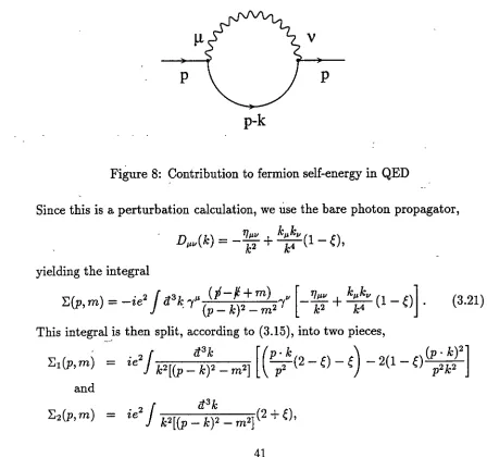
6 Fermion DS equation in QED 38 7 Photon vacuum polarization in QED 40 8 Contribution to fermion self-energy in QED 41

9 Contributions to the vacuum polarization. 58

10 Contribution to the fermion self-energy. . . 58

"As far as we can discern, the sole purpose of human existence is to kindle a light

in the darkness of mere being."

- Carl Jung

"The proof that the little prince existed is that he was charming, that he laughed,

and that he was looking for a sheep. H anybody wants a sheep, that is a proof

that he exists."

- The Little Prince, Antoine de Saint-Exupery

"Everything that happens once can never happen again. But everything that

happens twice will surely happen a third time."

- Proverb

"'Yes,' said the ferryman, 'it is a very beautiful river. I love it above everything.

I have often listened to it, gazed at it, and I have always learned something from

it. One can learn much from a river.'"

- Siddhartha, Hermann Hesse

"There's more to you young Haroun Khalifa, than meets the blinking eye."

- Haroun and the sea of stories, Salman Rushdie

"The most wasted of all days is that on which one has not laughed."

" ... the river is everywhere at the same time, at the source and at the mouth, at the waterfall, at the ferry, at the current, in the ocean and in the mountains, everywhere, and ... the present only exists for it, not the shadow of the past, nor the shadow 'of the future"

- Siddhartha, Hermann Hesse

"The best way to know God is to love many things." - Vincent van Gogh

"That's right. When I was your age, television was called books." - The grandfather in 'The Princess Bride'

"It

seems to me, Govinda, that love is the most important thing in the world.

It

may be important to great thinkers to examine the world, to explain and despise it. But I think it is only important to love the world, not to despise it, not for us to hate each other, but to be able to regard the world and ourselves and all beings with love, admiration and respect."

- Siddhartha, Hermann Hesse

"He didn't fall? INCONCEIVABLE!"

"You keep using that word. I do not think it means what you think it means."

Vizzini and Inigo in 'The Princess Bride'

Chapter

1

Introduction

The purpose of this introductory chapter is to place the subject matter of this

thesis within a historical perspective. We begin by outlining the progress made

in the analysis of field theory in three dimensions, then give a review of the gauge

technique, the non-perturbative technique we will exploit where necessary in our

calculations. The structure of the thesis is outlined in the final section.

1.1

Field

Theory

in (2+1)D

When studying gauge theories, it seems natural to look at a theory set in 3

+

1

space-time dimensions, as the physical world is set within such a geometry.

Ex-tensive research has been conducted on such theories, with considerable success.

Quantum electrodynamics is the simplest gauge theory to be physically

mean-ingful, describing the quantized interactions of photons and electrons. It is an

abelian theory, being described by the group U(l), and was found to be renor- / malizable

[1-3],

requiring only two renormalization constants [4]. In the

non-abelian case, the electro-weak or SU(2) x U(l) gauge theory [5,6] together with

spontaneous symmetry breaking

[7-9],

unifies the electromagnetic and weak

in-teractions, and also places a self-consistent theoretical framework around all of

the phenomenological weak models. Renormalization has permitted the terms in

intermediate vector bosons

[11-13]

has given the theory its necessary verification.

Another successful theory in

(3+1)D

is quantum chromodynamics

(QCD) [14-17].

QCD

is the gauge theory of the SU(3) colour group, and is largely accepted as

the theory describing the strong interaction. It provides a theoretical foundation

for the quark model

[18-21]

and can be used to explain the results of deep

in-elastic scattering

[22-24].

It is not considered as successful as the above theories

as it has so far been unable to supply a convincing explanation of confinement,

which is the process preventing the detection -of single quarks or coloured

par-ticles. It is possible that some insight may be gained by considering a theory

set in 2

+

1 dimensions. As well as having intrinsically interesting features, it is

thought that a

(2+1)D

theory could be used as a "toy" model to study the

con-finement problem

[25].

The bound state spectrum of electrodynamics in

(2+1)

dimensions has been studied, and the Bethe-Salpeter equation for the bound

states has been solved using the quenched ladder approximation and shown to

display confining behaviour

[26].

Also, the

(2+1)D

theory is known to display the

finite-temperature behaviour of the corresponding

(3+1)D

theory

[27,28].

In-any

case, electrodynamics in

(2+1)D

should be applicable to electrodynamic surface

effects.

Field theory in

(2+1)

dimensions displays many unusual properties. They can

be unique to

(2+1)D

and also quite at odds with our preconceptions from

(3+1)D.

First, in

(2+1)D

the statistics are arbitrary

[29-31].

This is because in two space

dimensions the particle configuration space is multiply connected, so when two

particles are interchanged, the wave function need not change phase by integer

multiples of 7r, as they must in

(3+1)

dimensions. Such particles are known

as anyons

[29, 30, 32, 33],

and will be discussed presently. For massless particles

in

2+

1 dimensions, spin is also arbitrary

[34, 35].

Since spatial rotations have

only a single generator,

J

3 , the algebra

[J

3 ,

J

3 ]

=

0 cannot lead to any obvious

quantization. Another peculiarity that we encounter is that in odd dimensions

parity is different. Since we have an even number of spatial dimensions, the

instead we must define parity as inversion of all but the last spatial coordinate [35].

It is this which leads to parity-odd objects, such as the gauge invariant

Chern-Simons term, which as we will see has a profound effect on our theory.

The simplest theory to consider in (2+ 1) dimensions is just quantum

elec-trodynamics, beginning with the usual

Fµvpµv

Lagrangian. The problem is that

when we undertake perturbation calculations, we encounter infrared (IR)

diver-gences. When experienced in (3+ 1 )D, this "IR catastrophe" [36] is handled by

also considering processes which include the emission of soft photons. The

"catas-trophe" becomes untenable in (2+ 1 )D, as it introduces nonanalytic divergences,

intractable within perturbation theory.

We can understand why such IR divergences arise in (2+ 1 )D by considering

a free field theory in 2+1 space-time dimensions,

where typically </> is a scalar, 'ljJ is a spinor and

Fµv

=

OµAv - OvAµ

is a Maxwell

gauge field. The dimensionlessness of the action (in natural units) specifies the

mass dimensions of the fields,

and with interaction Lagrangians like

(1.2)

we find that for

D

=

3, the coupling constant e has dimension [e] ,...,

M

1

₁

2_{• A}

renormalizable theory is one which has only a finite number of divergent Green's

functions. Electrodynamics in (2+1)D is called a super-renormalizable theory

since its coupling constant e has units of vfiii,, so since the perturbation

expan-sion is in terms of powers of e2

, higher-order diagrams -become necessarily less

ultraviolet (UV) divergent, resulting in only a finite number of UV divergent

di-agrams. This very feature, which minimizes the need for renormalization of UV

higher-order terms must result in terms containing higher powers of coupling

constant divided by higher powers of external momentum. Subsequently, when

calculating some further diagram which contains the first result as a subgraph,

and attempting further momentum integrations, the inserted result with a high

power of momentum in the denominator will add to the degree of IR divergence

of the momentum integral, leading inevitably to IR divergences. It was as a

re-sult of this failure by perturbation theory to handle this IR "catastrophe" that

researchers turned to non-perturbative techniques.

Cornwall and co-workers [38, 39] made one of the first attempts to overcome

this difficulty. To begin with, they considered a version of the theory where the

gamma matrices were parity-doubled 4 x 4 matrices. This meant that instead of

using the ordinary 2 x 2 gamma matrices, which would have resulted in fermions

whose masses violate parity, they embedded two species of fermions,. with mass

terms of opposite sign, into 4 x 4 matrices, restoring the parity invariance of the

massive Lagrangian. They then used the gauge technique ansatz [40] to solve

the Dyson-Schwinger equations [1,41-43] giving the gauge technique equation for

the fermion spectral function. They evaluated the fermion self-energy

perturba-l

tively, i.e. with a bare photon propagator, found an initial approximation for the

propagator, then obtained a finite solution which now broke the chiral symmetry "::

of the theory. It has since been found [44] by comparing this theory with the

2 x 2 version (see below) [37, 45, 46], that the zero bare mass demands 'P and

T

conservation, forcing this chiral symmetry breaking solution to be discarded.

Jackiw and Templeton [37] took a different approach. They resorted to using

the ordinary 2 x 2 gamma matrices, which are proportional to the Pauli spin

ma-trices, and studied massless fermions to avoid generating a photon mass. They

found that in order to stop the IR catastrophe from occurring, the photon

propa-gator needed to be "softened" , that is its IR behaviour needed to go from being

of 0(1/k2) to 0(1/k). Instead of using the bare photon, they considered the Dyson-Schwinger equation for the photon. This equation relates the full photon

any chosen order of expansion. By truncating at a suitable level and obtaining an approximation which permitted intermediate states to influence the photon's behaviour, they were able to obtain an IR finite answer. Their method was ef-fectively allowing the photon to be "clothed" in a cloud of massless fermions, moving outside perturbation theory by generating terms which were non-analytic in e. Guendelman and Radulovic and others, using both perturbative [47,48] and non-perturbative [49] techniques, also sought to_ avoid these IR problems by dressing the photon propagator. They also wished to avoid the occurrence of terms that were non-analytic in e2_{• To this end they exploited the residual gauge}

degree of freedom to eliminate the leading IR poles, resulting in a loop expansion which was analytic in the coupling constant. They found a limitation in their approach, however, since the ~xtra vector field introduced by them was not

suf-ficient to cure all the IR divergences, and quartic and higher-order terms in that ,, vector field would need to be introduced at higher orders.

Practitioners of the ~adder or

l/N

expansion (where

N

is the number of fermions) also considered this problem [27,28,50-54], applying their non-perturb-ative scheme to it. By resumming the expansion in terms of

l/N

they found that the IR behaviour of the photon was softened and the theory rendered IR finite.

- ; ; - -

-The problem was that this ·1/N technique attempts to solve the DS equations in -' their nonlinear form, making analytic results at even the lowest order extremely

Del-bourgo [57] considered the problem in a more systematic way, and were able to obtain an IR finite solution, without the need of any extra terms involving powers

of vector fields. The solution obtained contained the lowest-order perturbation

theory results within it, and gave the exact IR behaviour in the scalar and spinor

versions of the theory.

Several of the calculations described above could have allowed fermion masses

into the theory, since it is possible to introduce such parity-conserving fermion

masses when considering the form of the theory exploiting the doubled 4 x 4

gamma matrices, but in the work of Jackiw and Templeton [37] and Redlich

[45, 46], fermion masses would dynamically introduce a parity-violating photon mass term into the theory, which was, at the time, considered disadvantageous.

This parity-violating theory [58-61] has subsequently become the focus of a huge amount of interest. The theory exploits the fact that we can introduce directly

into the Lagrangian another gauge-invariant term of the form

Fµ.vAA EµvA ,

namely the Chern-Simons (CS) Lagrangian [62,63], which makes it topologically non-trivial. Several later works have gone on to consider the pure CS theory, that

is, CS theory with no Maxwell term present. This theory is found [64, 65] to be exactly soluble and to permit an understanding of the Jones polynomial [66,67] of knot theory in (2+1)D. The observables of this theory are Wilson lines, and the vacuum expectation values of these Wilson lines can be used to define link

poly-nomials [64, 68-71]. Further, these results have been used to explore conformal field theory (CFT) in 2D. For a CS theory defined on a compact 2D space, the

states in the Hilbert space correspond to the conformal blocks of the appropriate

2D rational conformal field theory [64, 72-74]. Another correspondence has been found, namely that the CS gauge theory is equivalent to the current algebra of

the CFT [64, 75, 76]. This connection can then be used to classify 2D CFTs, since any CFT can be obtained by selecting the appropriate gauge group of the CS

theory, and it has been conjectured that all conformal theories can be classified

One of the interesting features of field theory in (2+ 1 )D is that it allows for the existence of particles with generalized statistics, known as anyons [29, 30, 32, 33]. The possibility that such particles may actually exist led researchers to consider their possible applications. It was found that anyons were precisely what was needed to explain the excitations with fractional statistics observed in the fractional quantum Hall effect [77...:...79]. It has also been suggested [80-82] that anyons possess some of the attributes of high Tc superconductors. The

quantum mechanics of anyon systems is precisely described in terms of CS gauge theory [83, 84].

The study of gauge theories such as CS theory often lead us to the calculation of momentum integrals, and one is then confronted with UV divergences. These divergences are overcome by the use of a regularization scheme, which identi-fies singularities in an explicit form. There are several schemes which have been applied to CS theory, namely Pauli-Villars regularization [60],.analytic regulariza-tion [85, 86], nonlocal regularizaregulariza-tion [87] and dimensional regularizaregulariza-tion [88-92]. This thesis will in part consider a new formulation of abelian CS theory which permits a consistent application of dimensional regularization [93].

1.2

_Th~_Gauge

Technique:

In this section we will outline -the gauge technique (GT), the non-petturb~tive technique we will adopt to help overcome the IR problems encountered in (2+1) dimensional field theory.

'

and they also managed to render vector electrodynamics (VED) renormalizable, which is impossible within perturbation theory. Strathdee went on (99] to use the GT to explore non-perturbative behaviour in spinor electrodynamics (QED). The problem with the GT at this stage was that since the DS equations remained in a non-linear form, it became difficult to obtain analytic solutions at higher orders, so the technique remained largely unexploited. It was not until 1977 that Delbourgo and West (40] reformulated the GT, using the Lehmann spectral representation [100-102] for the fermion and the WGT identities to obtain a simple ansatz for the 3-point photon-amputated Green's function which amazingly rendered the DS equations linear, resulting in the first-order GT equation for the fermion spectral function in covariant-gauge electrodynamics. They obtained a solution of this equation in the Landau gauge, and Slim [103] subsequently obtained a

solution for an arbitrary covariant gauge. These successes, and the fact that the · 1

GT yielded almost trivially the exact IR behaviour in QED, SED and ,VED in covariant gauges [104, 105], prompted extensive research into applications of the GT.

The gauge properties of the GT solutions in (3+ 1 )D were studied by Del-bourgo and Keck [106], Slim [103] and DelDel-bourgo, Keck and Parker [107], using the Zumino identity for two-point Green's functions to obtain a relationship be-tween the spectral function in different gauges. It was found [106] that in SED, the solution obtained using this gauge covariance relation for the spectral func-tion, and that obtain:ed by the GT in an arbitrary gauge agreed precisely. In QED however, the spectral functions obtained from the GT only satisfied the co-variance relation in the asymptotic limits [103,107], violating the Zumino identity at intermediate momenta (in sharp contrast with perturbation theory), thought to be due to the neglect of transverse amplitudes.

Gardner [109], who found that the naive ansatz was no longer consistent, and so introduced a transverse component to solve the problem. Delbourgo and Thomp-son [110] then showed that this transverse part of the ansatz was unique and com-plete in (l+l)D. They went on to study the Thirring model, which showed that it is possible to apply the GT to a non-gauge theory, as long as it possesses gauge-type identities. Thompson also applied the GT to a (l+l)D axial model [111], where a complete solution was possible. The GT has also been used to address the question of dynamical symmetry breaking in various models (112-114]. The results have agreed with those obtained by other methods (115], with the benefit that the GT managed to avoid the divergences found in these methods.

Given these successes in various abelian theories it is natural to want to use the GT in QCD, where non-perturbative effects ar~ known to be important. The difficulty is that the GT utilizes the simplicity of the abelian WGT identities and the Lehmann spectral representation to obtain a very simple ansatz. In the

non-abeli~ theory, the generalizati<;m of the WGT identities, the Slavnov-Taylor (ST) identities (116, 117] are more complicated, as they are influenced by the presence of ghosts. Their form, which is no longer a simple difference of propa-' gators, is not suitable for constructing the GT ansatz. This difficulty has been

overcome most successfully [118-121] by considering that any physical process, ·y

such:. as quark,

sc~ttering

via a single gluon exchange, must be gauge-invariant. This implies that if we were to consider all contributions to the gluon self-energy, including those which appear to be of higher-order such as multiple-gluon emis-sions from a single point, the "self-energy" resulting from this resummation would be gauge-invariant. Obtaining resummed propagators and vertices in this way, it can be shown [118, 121] that since the gauge dependence has become trivial (only persisting in the bare gluon propagator), the ST identities become abelian-like, which allows the GT ansatz to be constructed. This technique, the so-called pinch technique, has been used to show interesting features within QCD, such as

,

Despite all these successes of the lowest-order GT, there remained a limitation. When considered to only this order, it did not allow for the determination of the transverse components of vertices. This limitation had been noted and expounded upon by many researchers. In the IR region it is no limitation, since transverse effects disappear in electrodynamics at least, but in general these contributions need to be considered. In (3+1)D spjnor electrodynamics, the renormalizability of the GT equation was not apparent, and it had been conjectured [122, 123] that transverse corrections would remove the divergences. It was also thought that the non-gauge-covariance of the spectral function in spinor electrodynamics was due to the absence of these transverse components. This led to the consideration of an extension to the GT, which began when King [124] modified the ansatz in

the spinor theory, introducing a transverse part. Beginning with perturbation theory, and being correct asymptotically up to leading logs, the transverse vertex refined the GT. Standard results were obtained in the asymptotic region, but the refined GT was still unable to reproduce

0(

e

4

) perturbation theory. In search

of a more sati.sfactory way of improving the GT, Parker [125, 126] considered a new approach. Looking at the scalar theory, the DS equation for the three point function was used as the starting point and a non-perturbative transverse vertex constructed which was consistent with perturbation _theory and correct in any momentum region. The only limitation with this technique was that it was valid only for the Feynman gauge, and that it incorporated an arbitrary constant. Delbourgo and Zhang [127, 128] completed the refinement of the GT. They managed to generalize the work of Parker to be valid in arbitrary gauge, and also to encompass the spinor theory. Their new GT equations were finite, linear in the spectral function, exact to O(e4

) in any gauge, had no ambiguous

I.

1.3

Structure of the Thesis

This thesis consists of six chapters, the first of which is an introduction to field

theory in 2+ 1 dimensions and the gauge technique.

The main body of the thesis begins in Chapter 2, where a scalar version of

elec-trodynamics in (2+ 1

)D

is considered. A framework is established which permits

both perturbative and non-perturbative study of the theory. The perturbation

approach is seen to be deficient in handling the infrared woblems inherent in

such theories, so the gauge technique is used as a non-perturbative tool to study

the theory. It is found that only by dressing the photon propagator [37] can an

infrared finite result be obtained. In order to understand the gauge properties

of the resulting meson spectral function, the gauge covariance relation (which

links the function in different gauges) is obtained, which confirms that the meson

spectral function is indeed gauge-invariant.

In Chapter 3, the full spinorial version of QED is considered, and the calcu-lations of Chapter 2 are repeated in this theory, with similar findings. We are

once again required to adopt a non-perturbative approach and dress the photon

propagator in order to obtain an infrared finite result. The gauge behaviour of

the resulting fermion spectral functi9n is once again explained by deriving gauge

covariance relations in the spinor theory.

. .

Chapter 4 begins our study of theories which permit the notion of parity

violation. . In the presence of a Chern-Simons term in the Lagrangian we see

that even techniques such as dimensional regularization, which seem universally

applicable, have difficulty being applied. We_ forego the usual naive "solution" to

this problem·, which involves an unnatural splitting of the D-dimensional space,

and instead develop a reformulation of the theory which exists in 21+1 dimensions

and is consistent for arbitrary l, so that dimensional regularization may safely be applied. The perturbation expansion is considered and we find that in contrast

to the previous two theories, Chern-Simons theory is infrared stable, enabling, the

Dynamical mass generation is the topic of Chapter 5. We consider in detail

the effect of a mass term which violates the parity invariance of the theory. It is

found that the presence of either a fermion or photon mass in the initial theory

will engender the other when quantum corrections are considered. These ideas are

then generalized, by considering the effects of parity-violating terms in arbitrary

odd dimensions. The induced topological mass term is calculated in arbitrary odd

dimensions, and interestingly, the purely topological theory in odd dimensions

greater than three is found to be distinctive in that no one loop fermion mass is

generated, due to the absence of a bare propagator for the photon.

Finally, Chapter 6 is made up of a summary of the thesis together with

sug-gestions for further study.

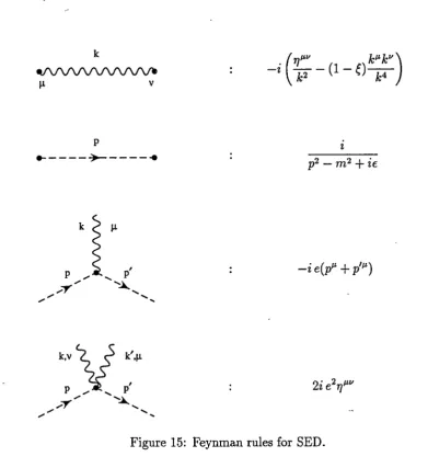
In addition, at the end of the thesis, several appendices are included, giving

the Feynman rules used, detailing some of the calculational techniques employed,

and discussing Dirac 1-matrices in odd dimensions. Reference is made to these

Chapter

2

Scalar Electrodynamics in

(2+1)D

This chapter will begin our study of gauge theories in 2+ 1 dimensions by consid-ering the electrodynamics of a scalar field. This theory has the advantage that it remains relatively simple, by avoiding the multiplication of terms encountered when taking the trace of products of 'Y matrices, as occurs in the spinorial version of the equivalent theory. We begin by detailing the formalism of Delbourgo [129], which considered the equivalent theory in (3+1)D, and make modifi~ations where .. neces~ary to apply_ the formalism to (2+1)D. We use this framework to study the theory using perturbation theory, and see explicitly the infrared singulari -ties encountered in such an expansion. Then we exploit the GT, which due to its non-perturbative nature is able to overcome these infrared difficulties. Fi-nally we study the gauge covariance rela_tions of the spectral function, to try and understand its gauge (in)dependence.

2,,,1

Background/Introduction

electrodynamics (SED). The Lagrangian in this case-will be of the form

( [(8µ

+

ieAµ)<Pr[(8µ

+

ieAµ)<P]

~

m

2

<Pt<P-

~pµv

Fµ

11 )

+

2_(8µAµ)

2

4 2e

- Co+ LaF, (2.1)

where

<P

is the scalar field,

Aµ

is the gauge field and

pµv

=

aµ A

11

-

8

11

Aµ

is the field strength. The last term in (2.1), the gauge-fixing term LaF, is introduced to

eliminate the residual gauge degrees of freedom of the action, and so permit the inversion of the gauge field propagator. From (2.1) we can generate the Feynman rules of the theory by taking functional derivatives of£ with respect to the fields. For example, the (inverse) gauge propagator is

n-1

_µv

s2.c,

8Aµ8A

11

-

-TJµvk

2

+

(1 -

e)kµkv,

. (2.2)

which may now be safely inverted. This is done using the condition that the product of the propagator and its inverse should result in

T/µv·

Selecting a propa-gator consisting of all possible two-index tensor forms, each carrying an unknown constant, then solving for these constants, we obtain

(2.3)

Similarly, the meson propagator and the meson-meson-photon vertex can be de-termined. The complete set of Feynman rules for SED is given in Appendix

A.

Since this is a gauge theory, we must ensure that we preserve the gauge sym-metry. One way to do this is via the Ward-Green-Takahashi (WGT) identi-ties [96-98] connecting successive source Green functions. The WGT identities can be derived by considering the effect of a set of transformations on the gen-erating functional,

W[J].

We can see that £0 in (2.1) is invariant under these

Aµ(x) ---+ Aµ(x) - 8µA(x)/e

<P(x) ---+ <P(x)

+

iA(x)<P(x)

<Pt(x) ---+ <Pt(x) - iA(x)<Pt(x),

where A(x) is a real infinitesimal scalar function. We consider the effect these transformations have on the generating functional W, which must also be invari-ant under them. If we define the action

S

as

(2.4)

where the source term Cs is given by

(where j'-', 17t, 17 are the sources of Aµ, <P, <Pt respectively) then the vacuum generating functional is

(2.5)

and further

W,

the generating functional of the Green's functions, is defined by

Considering the variation of the gauge-fixing and source terms (since !:::..£0 = 0),

and demanding the invariance of Z under this variation then implies

(2.6)

which is the fundamental functional gauge identity. In terms of Wit takes the

form

We take the Legendre transform of (2. 7) via

which relates the one-particle-irreducible generating functional

r

to W, resulting

lil

[8

2

8µ.Aµ-oµhT(x) of(x),1.( )- ,1,.f(

)of(x)l

=

e

z SAµ

+

e o<f>( x) 'f' x e'f' x o<f>t( x) O. (2.8)

This contains all the information we need to obtain any of the WGT identities

I

within this theory. To obtain the WGT identity which involves the meson propa-gator, we need to take the functional derivative of (2.8) with respect to

</>(x)

and its conjugate, i.e St/J(Yl;.Pt(z), which yields

Now we need to make the identification that SA,.(:z:):;[u)sq,t(z)

=

fµ(x;y,z) is the

full photon-meson-meson vertex and sq,(rj~~t(y)

=

_b.-1(x,y) is the inverse meson propagator, so our relation becomes

Finally, transforming this to momentum space, we obtain the familiar expression (2.9) Similarly, by taking suitable functional derivatives of (2.8) al;>ove, we may derive WGT identities for the photon :field and higher-order Green's functions.

By choosing a function which satisfies its associated WGT identity, we pre-serve the gauge symmetry of the theory. It is possible to begin with the lowest order WGT identity in its usual form, (2.9), then solve for

r

µ in terms of _b.-1.

This is the technique used in the original references on the GT (94, 95, 99, 122) and by Ball and Chiu (130, 131) and subsequent workers (132-134). The problem with this approach is that it produces a nonlinear equation for b. -1. When substituted

the ladder approximation, which is a severe limitation. Instead we follow

Del-bourgo

[129]

and manipulate equation

(2.9)

by multiplying it on the left by

.6.(p)

and on the right by

.6.(p - k),

giving us

kµ

.6.(p)r µ(P, P - k).6.(p - k)

=

.6.(p - k) - .6.(p).

(2.10)

In order to set up an iterative way of solving for the particle propagators, we will utilize the Lehmann spectral representation of the meson

[100-102],

namely

.6.(p)

=Joo

e(w)dw ..

-oo

p2 - w2

+

ie

(2.11)

We use this form of dispersion relation rather than the conventional

as the spectral function in three dimensions naturally takes a form involving

#,

as will become apparent. By observing that the difference

J

(2p -

k)µkµe(w)dw

.6.(p- k) - .6.(p)

=

(p2 -w2)[(p- k)2 - w2]'

(2.12)

Delbourgo

[129]

saw that a very simple, though not unique, solution of

(2.10)°

is

,

to take the longitudinal Green's function as

J

(2p - k)µe(w)dw

.6.(p)r µ(p,p - k).6.(p - k)

=

(p2 -w2)[(p- k)2 - w2)"

. (2.13)

It is clear that this is exact only up to an arbitrary transverse function, which

could be added to

(2.13)

without violating the gauge identities, since any

trans-verse function will be annihilated when contracted with

kµ.

Now, to find the lowest-order corrections to the bare propagators, we consider

the Dyson-Schwinger (DS) equations

[1,41-43]

for the propagators. We find it

convenient to work in momentum space, and if we assume

Aµ(k)

and

jµ(k)

are

then we can obtain the Fourier transform of the action

(2.4)

explicitly, giving S

=

j il3_{k [-!Fµ}

11(k)Fµ

11(-k) - kµkvAµ(k)A 11

(-k)

+

(k2 - m2

_{)</>t(-k)</>(k)}

4 ' 2~

-e j il3_{p (p - k)µ</>t(p)Aµ(-p - k)</>(k)}

+e2

J

a

3p

a

3p' <Pt (p )Aµ( -p - p' - k )Aµ(p')<P( k)

-qt(k),P(-k) -,Pt(k)q(-k)- i"(k)Aµ(-k)],

(2.14)

where we now adopt the convention that il3p

=

<f3p/(27r)

3_{, which we will use}

throughout this thesis. The

DS

equations result from the fact that the vacuum expectation value of the functional derivative of the action with respect to any of its field operators is identically zero, for example,

O = j[d</>d</>tdAµ]

(o</>~k)

exp[iS])

= _

j[d</>d</>tdAµ]

[(k

2

_ - m2

)</>t(-k) -

e j i13p(p - k)µ</>t(p)Aµ(-p - k)

+e2 j i13_pi13_{p'</>t(p)Aµ(-p-p' -k)Aµ(p')-17t(-k)l exp[iS]}

_.(2.15)

Noting from

(2.5)

that

and

i

ojµ(~Z+

k)

=

j[d</>d</>td4µ].{lµ(-p- k) exp[iS], we can express

(2.15)

as

(2.16) Equation (2.16) may be used to generate the DS equation for any photon-amp-utated Green's function G. For example, if we wish to generate the

DS

equation for the meson, we take the functional derivative of (2.16) with respect to

77t(q).

We then set the sources to zero, and note that

due to the absence of spontaneous breaking of charge symmetry or Lorentz in-variance. This results in

(2.17) We now define the (n+2)-point unrenormalized Green's function (with n external photon lines) by

(T:rr )µ.1 .. ·JJ.n( ' . )c( ') _ ·nH 8n+

2

W[O]

"" u p ' •.. , p, •.• u p

+ ... -

p - z c (- ) c t( ) c . c . ' U'1] p' U'1] p _{U}µ. 1 • • • UJµ.n}

in terms of which (2.17) becomes (after integrating out the 8 functions)

1

=

(k2-m5).6.u(k)

+

ieoja

3p(p-k)v(Wu)11

(k,p)

+

ie5.6.u(k)

Ja

3pgµ.v(Du)JL"'(p)

-ie5

J

i!3p

a

3p1

gµ.v(Wu)µ.11

(p,p1

where the u subscripts denote unrenormalized quantities. We wish to write this in

terms of the photon-amputated Green's functions, G

=

.6.f .6., which are defined by

(TAT

"" v.

)µ1···µn(

p ' ... 'p, ...

I • ) " ( 0

p

+ ... -

p -

' ) _

·n+3(

)n(D )µ1111

(D )µnlln(G )

(

I )

Z -eo u • • • u u

11

1 ...

11n

P · · · P · · · ,

and using this we obtain

1

=

(k2 -

m~).6.u(k)

-

ie~

j

a

3

p (p- k) 11 (Du)µ

11(k - p)(Gu)v(k,p)

+ie~.6.v.(k)

j

a

3

_{p gµ 11 (Dv.)µ}

11 (p)

(2.19)

+eci

f

a

3

p a

3

p'(Dv.t°'(p')(Dv.t13 (k-p-p')( Gu)a13(p, p', k-p-p'; k ).

If we renormalize this equation multiplicatively, using

and write it in terms of the vertex functions (or f's), we achieve the meson DS

equation given in (2.21) below. A similar approach would also yield the photon

DS equation.

The DS equations are not part of perturbation theory, as they involve full

propagators instead of a bare loop expansion, but they are consistent with it "

to any order of expansion in e, and the lowest-order perturbation result can be

regained by putting

e<

0

_>(w)

₌

_{8(w - m). We adopt this form only to allow a}

consistent approach in the next two sections. The first in the infinite series of

complete DS equatio_ns for the photon reads

n;:(k)

=

(-TJµ11k

2

+

(1-

e)kµk 11 )ZA

+

2ie2Z

J

T/µ 11.6.(p)a

3

p

-ie2

z

j

il3

_{p .6.(p}

_)r

_{µ(p, p - k ).6.(p - k )(2p - k )11}

+2e

4

z

j

_.6.(p

_)r

_{1t11(P, k; p', k').6.(p')D:( k')a}

3

_pa

3

_p'

_ -(-TJµ 11k

2

+

₍₁

-e)kµ.k11 )ZA

+

ITµ11(k),

(2.20)

where Z is the source renormalization constant, ZA is that of the photon and

r

µ

11

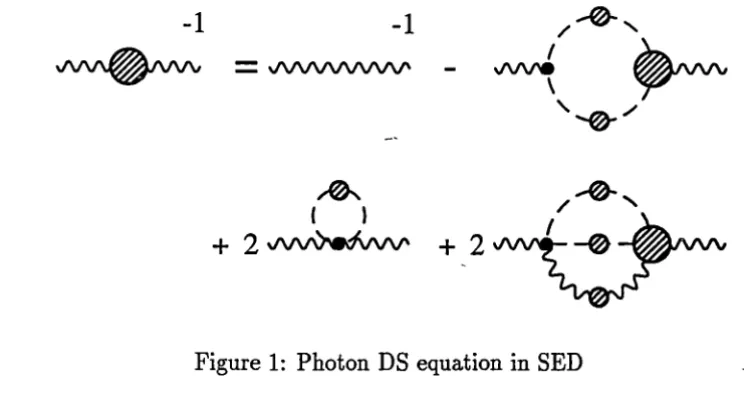
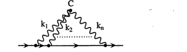
stated. We may also represent equation (2.20) in terms of Feynman diagrams, which we do in Figure 1 below.

-1

-1

~

=

VVVVVVV\/V'

~

I I

+

2

vvWw<fvvv.

+

2

Figure 1: Photon DS equation in SED

In Figure 1, (and Figure 2 below) a wavy line corresponds to a photon, a dashed line represents a meson, a dot corresponds to a vertex, and a shaded "blob" indicates that the propagator is regarded as full, i.e. exact to all orders. Similarly, the lowest DS equation for the scalar meson (assuming for the present that it h~s

a non-zero bare mass m_{0 ),} is

Zi

1 =

(p

2

-

m5).6.(p) -

ie2

J

iJ

3

k .6.(p)f v(p,p - k).6.(p- k)D

1

w(k)(2p-:- k)µ

e• _ ·-· • •

+~e

2

.6.(p)

j

D,f(k)i1

3

k-...

_.~ ~

. _ _ _

_ ...

+2ej

.6.(p)f

µv(P, k;

p~p+p'

+k).6.(p+p'

+k)Dµ>.(k)Dv>.(k')i1

3

p~

3

p~

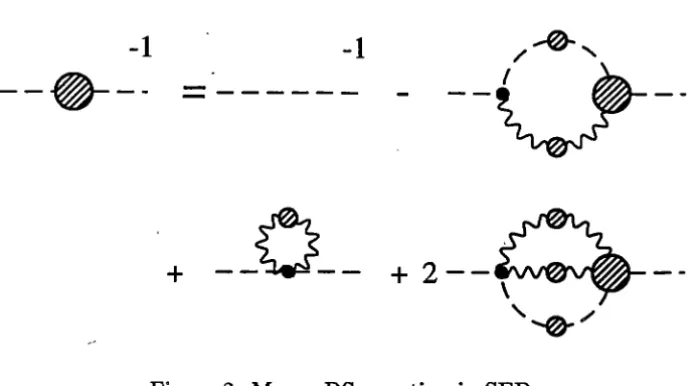
(2.21) which may also be 'represented diagramatically, .as shown in Figure 2.

These equations hold to all orders, since they involve the full propagators and vertex functions, making them potentially very powerful. Within this frame-work, that is,· using the ansatz (2.13) to linearize the

DS

equations, the photon polarization is given by

• 2

j ()

J

3 [

(2p-)•)µ(2p-k)v

2'f/µv]

ITµv(k)

=

-ie

Z {]

w dw il

P

(p2 _ w2

)[(p-

k)2 -w2] - p2-w2 (2.22)

[image:30.565.113.485.137.334.2]

-1

--·--

-1

--0--__ o --0--__

+2--A---,

...

+

Figure 2: Meson DS equation in SED and the meson propagator obeys the equation

z;t -

(p2 - m~)~(p)

-! (

)d .

21

il3k [(2p - k)µ.(2p - k)vflP.V(k) _ D

"'(k)l

f1 w w ie (p2 - w2)[(p-k)2 - w2] µ.

+

2-photon - 1-meson terms

(p2 -

m~)~(p)

+

j

e~w)~L:(p,w),

p -w (2.23)

or, upon using the renormalization condition m_2

=

m~ - :E(m,m) [122] we find 0

=

J

w2 - m2

+

L:(p,w)

~

L:(w,w) e(w)dw.

p2 _-w2

+

_ic (2.24)

Since this :E is still the full meson self energy, we must be careful in taking the imaginary part of (2.24). If we are taking the discontinuity of some integral

J

dw J(w)

p2 -w2'

then we obtain two contributions,

J

dw p2 -w2

SSJ(w)

and

j

dw~f(w)o(p

2

-w2).

Returning to (2.24), we find that

SS[/

L:(p,w) - L:(w,w)

aw]

= Jaw:E1(p,w)

-f

dw:E1(w,w)

p2 _ w2 p2 _ w2 p2 _ w2

+

J dw[L:R(p,w) - L:R(w,w)] O(p2

[image:31.566.138.488.76.269.2]

where

E1

=

~~E(p,

w)

is the discontinuity of the meson self energy for a mass

w

meson, and ER

=

~~E is its real part. The second integral on the right hand side is obviously zero, since we know that the self-mass E(m, m) is real, and the final term will not contribute since the 8 function will cause its two parts to cancel.

This means we may write the imaginary part of (2.24) as

(p2 - m2)

J

e(w)dw

2

#

_p

e(p)

= _p 2 _-w 2

E1(p,w).

(2.26)

We now have the necessary tools to permit the consistent study of SED using both perturbative and non-p-erturbative techniques. We will begin ,in the next section, by considering perturbation theory.

2.2

Perturbation Theory

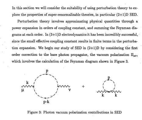
In this seCtion we will consider the suitability of using perturbation theory to ex-plore the properties of super-renormalizable theories, in particular (2+1)D SED.

Perturbation theory involves approximating physical quantities through a power expansion in orders of coupling constant, and summing the Feynman dia-grams at each order. In (3+1)D electrodynamics it has been incredibly successful,· since the small effective coupling constant results in finite terms in the perturba-tion expansion. We begin our study of SED in (2+ 1 )D by considering the. first - · order correction to the bare photon propagator, the vacuum polarization IIµ11 ,

which involves the calculation of the Feynman diagram shown in Figure 3.

p

-~ ...

,,...

'

/ \

k

I \

~

Wvvv

µ

.

I V

\ I

\

'

_... ~_,,,,,,, -~/

p-k

+

.2 ...

/ \

I I

\ I

~

k

k

[image:32.565.61.528.354.748.2]

As intimated in the previous section this perturbation expression is equivalent to setting e(o)(w) = 8(w - m) in (2.22), giving

II (k)

= _ ·

2

J

i13 [(2p - k)µ.(2p - k)v - 217µ.v[(p - k)2 - m2]]

µ.v

ie

.

P (p2 _

m2)[(p _

k)2 _

m2]

·

(2.27)

We wish to explore the UV convergence of this integral, which we can do using power counting. This is a method of seeing the superficial degree of divergence of an integral by comparing the power of momentum in the numerator and de- c'

-- nominator. If the total power of momentum in the numerator (allowing for the dimension of the momentum integration) is larger than that in the denominator, then at large momenta the integral will diverge, whereas a larger power of mo-mentum in the denominator will have the converse effect, yielding a UV finite result. It can be seen that in the above integral, equation (2.27), the effective mo-mentum is (3+2)-4

=

1 so the numerator dominates, and the integral appears to be UV divergent. A regularization scheme is required to evaluate the momentum ,integral, and render any residual singularities into an amenable form, ready for

renormalization techniques. We choose dimensional regularization [135-139], for several reasons. First, it is convenient, since any infinities encountered appear simply as poles in

r

functions. Also, it is simple to use, since the propagators retain their inverse quadratic form, making the integrations relatively easy· to compute. Finally, it preserves the gauge invariance of the theory, which is vital if results in a general covariant gauge are required. The technique of dimensional regularization is outlined in Appendix B, where (2.27) is evaluated explicitly, g1vmg

rr ••

(k)

=

-

1

~:(-q

..

+

k~:·)

[4m

+ (

#-~)In

G:

~ ~)

l ·

(2.28)

Notice that the rE:'.sult is strictly finite, which is ensured by gauge invariance. If we study the asymptotic behaviour of (2.28) we see that, provided m =/:-0, as k ~ 0, II tends to e2k2 _{/67rm, and otherwise it equals}

-e

2

~/16.

_{Alternatively, it}

also yields (2.28). It will be useful to incorporate this photon self-energy in the full photon propagator via a dispersion relation

(37].

We do this by finding an asymptotic approximation of (2.28) valid both for k--+ 0 and k--+ oo and which becomes exact for m = O; explicitly

n-1

(

kµk11) (k2

~k

2 )

µ11 ~ - -TJµ11

+

k2

+

~?rm _

V-JC2 ·

(2.29) Taking the.discontinuity of the inverse of this equation yields

<;SD (k) - -(- kµk11) ( e2 3m?r 8(k2))

µ11 - - 17µ11

+

k2 16Jk2(k2

+

c2)

+

2c (2.30) h 3 e2Th .

w ere c = ₂?rm

+

₁₆• en, usmg

kµk11 [00 p(µ )dµ

Dµ11(k) = -(-17µ11

+

k2)

Jo k2 _ µ2 (2.31)

and noting that

( -11µ11

+ k2

kµk11)_( ) _ p µ =

-;-;.s

2µ~n µ11 ( ) µ

=

(-q_.

+

k~;') [c;~:,

+

3m (;c

8(µ) -

c'

~

µ')],

we obtain (up to a

ZA.

scale factor) the spectral representation (m

#

0) of the dressed photon propagator,

' kµk11 [(2c [00

dµ 1 3m?rl kµk11 ( )

.Dµ11(k) = (11µ11. -

k2) -;.-

3m) Jo k2 _ µ₂ µ₂

+

c2

+

_2ck2

-ek4.

2.32 . Note the dangerous pole at k2 = 0 is lurking in (2.32) when m

#

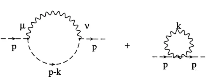
0.

We now turn to the meson self-energy, :E(p, m), within perturbation theory. This is equivalent to evaluating the Feynman diagram in Figure 4.

We obtain the expression for :E(p, m) from equation (2.23) by limiting ourselves to the bare photon propagator,

( ) 17µ11 kµk 11

Dµ11 k =

-/;2

+

°"k4(1 -

e),

(2.33) resulting -in the expression

:E(p, m) = -ie2

j

a

3k (2p - k)µ(2p - kY [- 11µ11

+

kµk11 (l _

e)]

(p-k)2-m2 k2 k4

_ . 2

J

:t3k 1

+

e

--+--p

v

~-\ I

p

' I

'

/

-~-"""

p-k

+

_Q__

p

p

Figure 4: Contributions to meson .self-energy in SED

The second integral in equation (2.34) obviously disappears in dimensional regu-larization, since within that scheme,

-if

iJ3k

=

k2

lim - .

a

3

_k(k2f

Tr;-_-,,i - z

J (

k2 - Af2)E

lim

(-1f-Er(l

+

T)r(E -

l-T) Tr;-.:-01 ( 47r

)lr(Z)r(E)(M2)E-l-T

0.

(2.35)

We now evaluate (2.34) using the techniques associated with dimensional regu-larization, yielding

_ e2

(p

2

+

m

2)

[m

+

#]

e

2

m

, E(p,

m) -

..Jij2

log

#

-2 , 47r p m - p 7r the imaginary part of which is

e2

Er(p,m)

=

H(p2

+

m2)0(p2 -

m2),

47r p '

where O(p2 _{- m}2

) is just the unit step function, defined by

O(x)

= {

~

x>O

x

<

0.

(2.36)

(2.37)

Notice that both (2.36) and (2.37) happen to be gauge independent in three dimensions. The explanation for this is given in Appendix C, where we summarize the relevant calculations in any dimension.

Since

Er

in (2.37) above is of order e2_{, equation (2.26) may be used iteratively}

to give the perturbation expansion for (}, taking the form

co

[image:35.563.129.467.71.202.2]

Putting the ith order expression for g in the right hand side of (2.26) will give the ( i

+

1 )th order term in the expansion on the left hand side If we now do this, by beginning with the lowest-order result,

g<

0

_l(w)

=

_{8(w - m), we arrive at the}

first order ( e2) spectral function

2 2

+

2

(1)( ) _ .:_ P m (

2 _ 2)

e

P - 27r

(p2 -

m2)2 0 P w . (2.38)

Attempting to carry out the perturbation expansion to the next order shows how things can go wrong if we do not allow for photon-line corrections in our

O(e

4

)

calculations. We are confronted with the following integral

(2.39) which is clearly divergent at both ends of integration, and near w = m we meet

the so-called "infrared catastrophe". In (2+1)D it is more like a "cataclysm" since unlike SED in (3+1)D, the divergence is not logarithmic but linear.

2.3

The Gauge Technique

In this section, we will consider non-perturbative methods to try to overcome this IR difficulty. The first alternative is that it may be possible to continue studying (2.26), but instead of a perturbation expansion, recast (2.26) into the form (m

=

0)

/2(2p)

=

j

Er(p,w]- E21(p,p) g(w)dw

+

Er(p,p)~(p),

p -w (2.40)

then try a power law selection of ~(p) to avoid the singularity. Equation (2.40) looks to be in a more well-behaved form, but our work suggests that this naive hope is unlikely to succeed as we find that a p

=

w singularity in the integration region persists.

identity in the form of (2.13) to determine the photon propagator, and go on to evaluate the meson self-energy using this dressed photon propagator. Evaluating

IIµv(k) from (2.22) we firstly obtain a non-perturbative estimate of the photon

self-energy,

·before attempting to determine the meson self-energy. Since as yet we know nothing about the non-perturbative behaviour of

e(w),

we will assume a finite mass m threshold as a starting point and put

e(w)

=

S(w -

m) to return to the perturbation result (2.28) for II. Later, having determined the behaviour of

e(w),

we may return to (2.41) to refine our result, since the dressing of the photon line is the only source of nonlinearity in the GT.

Let us see why the question of mass is so important in our calculations. As-sume for a moment that we take m =/:- 0, which means using the massive dressed

version (2.32) of the photon propagator. This would result in our meson self-energy taking the form

't""I(

)

= _.

2f

"'3k(2p-k)µ(2p-k)"

LJ p, m ze u ( k)_{2 2} x

p- -m

[ kµ.kv ( 2c {°" dµ 1 3m7r) _ kµkv] x (T/µ.v -

k2) (-;-

3m) lo k2 - µ2 µ2

+

c2

+

2ck2 -

~k4

'

which, after some calculation yields a- discontinuity

-e2 · _{2 2} e4 [7r(p2 _ w2)2 (p2 _ w2)2 E1(p,w) = 47rv9(3p

+

w )

+

327r2JP2

2c3

c2(

f f -

w)

+

(p2 w2 ( p2 w2" p2 w2

l

+ \

~

1 -

~

}) arctan(

~

) . (2.42) Notice that once again this result is gauge-invariant. Al~o, it is important to notice that only the first term in (2.42) lacks a factor of p2 _-w2

• _This means that

when we insert (2.42) into (2.26),-only this part will retain a factor of p2

- w2 in

spectral function has support away from the origin, the low-energy part of II will

still be proportional to

k2

and contribute to the photon renormalization constant

ZA without softening the k --+ 0 behaviour.

It seems that our only hope to effect a cure is to assume the existence of some

massless intermediate state in II. Let us therefore fix upon some scalar source

with renormalized. mass m

=

0, which clothes the bare photon propagator to

kµkv) 2c

1

00

dµ 1 kµkv

Dµv(k)

=

(TJµv - -k2 - k2 2 2

+

2 -J-k4 ;

7r 0 -µ µ c c = e

2

/16. (2.43)

Using such a dressed photon propagatora and dropping the 2-photon-1-meson

graphs which are separately gauge-invariant, our meson self-energy discontinuity

becomes

L:r(p,

w) e

2

c [ 2p2

+

2w2

+

c2

(H -

w)

2 r::::r arctan

47r yp2 c c

(p2 -w2)2 {7r

(H

-w)}

+

- -

arctan

c3 2 c

G.

(p2 - w2)2

l

2 2

+yp--w-

c2(vfr-w) O(p

-w ),

(2.44)

which once again remains independent of

e.

Notice that if we allow c --+ 0, we

find

. e2

L:r(p, w) ,....,

47r#(p2

+

w2)0(p2 -

w2),

which is exactly (2.37), so the perturbation theory result is still contained within

(2.44). More significantly,

L:r(p,p)

= 0, and this is an infrared panacea!

Return-ing to (2.26) we can now attempt to solve this linear equation for the spectral

function, which has the form

(2.45)

a More generally we easily see that the constant c = N e2

/16, where N is the total number

Due to the complicated nature of this equation a complete analytic solution isn't

possible, so we look at the behaviour in various asymptotic regimes. Since at IR

momenta, i.e. (

#, -

m) ~ e2_{, we may make the approximation}

(#-m)

H-m

(#-m)

3

(H-m)

5

arctan "' - c3

+

0 ₂ ,

c c 3 e

the self-energy becomes

which to leading order in

(p

2 _{- w}2_{) is}

and the equation,

p{!(p) ,....,

-e2 [P

e(w)dw;

2 7r2_c

Jo

is readily solved to give a spectral function for the meson which behaves as

(2.46)

Similarly, if we study the UV behaviour of (2.45) above, i.e. assuming (

#'-m) ~ e2, it is quite valid to make the approximation

(

# -

m) 7r c ea ( e2 )

5

arctan ,...., - -

+

+

0

,

c

2

# - m 3(#-m)

3

H-m

so that the self-energy takes the UV form

e2c [-(p2 + w2)7r

G

err

2(p2 + w2)

,....,

+(yp2-w)--+---==---- 47r2

#

_{c 2}

H-w

(p2 _

w2)2

c2

l

-(#-w)3

+

_{# - w ) '}

We now need merely to solve the eql!ation,,

. e(p) -e2

loP

p - "" - e(w)dw,

- 2 47rp 0

which yields the result

(2.4 7)

-We can see that in both momentum regimes the meson spectral function remains gauge-invariant.

2.4

Gauge Covariance Relations

In order to understand why the spectral function is gauge-invariant in both the GT and to order e2 _{in perturbation theory, we will now study the .general x-space}

behaviour of the spectral function following the technique of references~[106,107], ~·

yielding the gauge covariance relations in (2+1)D for the spectral function. We wish to determine the behaviour of our propagators under the gauge transforma-tion

(2.48)

-</> ~ <f>exp(ieA(x)).

We follow Zumino [140] (using his notation) and begin by considering the gener --ating functi~nal Z, which transforms via (2.48) as

or, in differential form,

.8Z -

(a

·µ

_§_

t~)

z

-z SA - µJ

+

e11 811 - e11 811t • (2.49) Let us consider the gauge changes corresponding to a change in the generating functional defined by