Improvement in Accuracy for Three
Improvement in Accuracy for Three
Improvement in Accuracy for Three
Improvement in Accuracy for Three----Dimensional Sensor (Faro
Dimensional Sensor (Faro
Dimensional Sensor (Faro
Dimensional Sensor (Faro
Photon 120 Scanner)
Photon 120 Scanner)
Photon 120 Scanner)
Photon 120 Scanner)
Mohd Azwan Abbas1, Halim Setan2, Zulkepli Majid2, Albert K. Chong3, Lau Chong Luh2, Mohd Farid Mohd Ariff2, Khairulnizam M. Idris2
1
Department of Geomatics Science, Universiti Teknologi MARA Arau, Perlis, Malaysia
2
Department of Geomatic Engineering, Universiti Teknologi Malaysia Skudai, Johor, Malaysia
3
Department of Geomatic Engineering, University of Southern Queensland, Australia
Abstract
The ability to provide actual information and attractive presentation, three-dimensional (3D) information has been widely used for many purposes especially for documentation, management and analysis. As a non-contact 3D sensor, terrestrial laser scanners (TLSs) have the capability to provide dense of 3D data (point clouds) with speed and accuracy. However, similar to other optical and electronic sensors, data obtained from TLSs can be impaired by errors coming from different sources. In order to ensure the high quality of the data, a calibration routine is crucial for TLSs to make it suitable for accurate 3D applications (e.g. industrial measurement, reverse engineering and monitoring). There are two calibration approaches available: 1) component, and 2) system calibration. Due to the requirement of special laboratories and tools to perform component calibration, the task cannot be carried out by most TLSs users. In contrast, system calibration only requires a room with appropriate targets. Through self-calibration, this study involved a system calibration for Faro Photon 120 scanner in a laboratory with dimensions of 15.5m x 9m x 3m and 138 well-distributed planar targets. Four calibration parameters were derived from well-known error sources of geodetic instruments. Data obtained using seven scan stations were processed, and statistical analysis (e.g. t-test) shows that all error models, the constant error (8.9mm), the collimation axis error (-4.3”), the trunnion axis error (-11.6”) and the vertical circle index error (8.0”) were significant for the calibrated 3D sensor.
Keywords: 3D sensor, terrestrial laser scanner, accuracy, systematic errors, self-calibration.
1. Introduction
Recently, three-dimensional (3D) model has been widely used for many purposes such as reverse engineering, medical, accident mapping, facility management, industrial measurement, monitoring and city modeling. In order to provide 3D information, there are several methods which can be used to acquire 3D data either using contact or noncontact scanners. Coordinates Measurement Machines (CMMs) is an example of contact scanner,
which is very popular among mechanical engineers. However, there is restriction on the size of the object part scanned and also it can be slow in data acquisition rate because each point is generated sequentially at the tip of the probe has become the main drawback of CMMs method [1]. The tacheometer is a noncontact based scanner which can give better accuracy but it’s not only slow and cumbersome (during data collection phase) but most of the time this method also fail to provide the amount of detailed required [2]. Photogrammetry also noncontact scanner can be used to obtained 3D data but it required extensive manual editing and refinement for modeling purposes. With the rapid increase in speed and accuracy, and capability to provide 3D data (point clouds) directly, terrestrial laser scanners (TLSs) make it much easier to produce 3D models. Furthermore, their costs and sizes also have been continuously decreased. For that reason, TLSs have been chosen by many researchers for 3D modeling applications.
argument arises because all electronic and optical instruments contain systematic errors. The precision can be determined by referring to manufacturer specification or by independent testing. Accuracy is different, it has to be evaluated through the deviation between the nominal and real value. In order to ensure the high quality of information provided by TLSs, calibration routine is very essential. Furthermore, the calibration process is very crucial to guarantee the data provided by the scanner meet the requirements of the job specifications.
Fig. 1 : Applications of scanner with respect to the measurement precision [3].
2. Terrestrial Laser Scanners
TLSs is a non-contact sensor, optics-based instrument technology that collects three-dimensional (3D) data of a defined region of an object surface automatically and in a systematic pattern with a high data collecting rate. This capability has made TLSs widely applied for robust 3D reconstruction. In order to capture 3D point clouds that covering its entire field of view, laser source direction should be changed during scanning process. This can be performed either by rotating the laser source itself, or by using a system of rotating mirrors. The latter method is commonly used because mirrors are much lighter, faster and gives higher accuracy. This method may consist of either two scanning mirrors or one scanning mirror and a servomechanism. There are three different types of beam deflection units used in TLSs (Figure 1) as follows:
i. Oscillating mirrors;
[image:2.595.55.285.223.327.2]ii. Rotating polygonal mirrors; and iii. Monogon (flat) rotating mirrors.
Fig. 2: Beam deflection units used in TLSs [6].
Figure 2 shows that the type of laser beam deflection unit which represents the field of view (FOV) of the TLSs. According to Staiger [5] and Reshetyuk [6], there are three classifications of TLSs based on FOV as follows (Figure 3):
i. Camera scanner; ii. Hybrid scanner; and iii. Panoramic scanner.
Fig. 3: Classification of TLSs based on field of view, (a) Camera scanner, (b) Hybrid scanner and (c) Panoramic scanner.
Camera scanner uses oscillating mirrors to deflect the laser beam about the horizontal and vertical axes of the scanner. The scanning head remains stationary during the scanning process. The system carry out their distance and angle measurement over a much more limited angular range and must be within a specific FOV (Figure 3a) of e.g. 40x40°, comparable to a photogrammetric camera [5].
Hybrid scanner has a horizontal FOV of 360° but a limited vertical FOV (Figure 3b). This scanner employs the oscillating or rotating polygonal mirrors (Figure 2) to deflect the laser beam in vertical and horizontal axes. With aid of servomotor, hybrid scanner is capable to be rotated by a small step around the vertical axis (horizontally). It works by scanning the vertical profile using a mirror system, and this process is repeated around the vertical axis until the scanner rotates a full 360°.
Monogon mirror used in panoramic scanner has improved the vertical FOV compared to hybrid scanner (Figure 3c). Using the same mechanism as hybrid scanner which is based on servomotor, this scanner is also capable of providing 360° horizontal FOV. These advantages of having a 360° horizontal FOV and nearly the same amount for vertical FOV has made panoramic scanner very useful for indoors scanning.
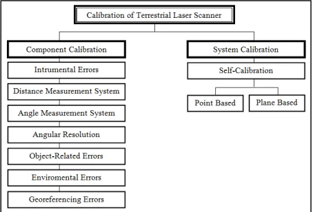
3. Calibration of Terrestrial Laser Scanners
[image:2.595.46.285.569.701.2]Fig. 4: Calibration procedures for terrestrial laser scanners.
2.1 Component Calibration
[image:3.595.61.286.452.560.2]According to Schulz [3], component calibration requires precise knowledge of the scanner error model, and individual error is investigated separately in a specific experimental setup. All of these errors are identified separately in component calibration. In order to carry out this type of calibration, special facilities and device are required (Figure 5). Other than being used for calibration purposes, component calibration also performed to compare the performance of scanners from different models and manufacturers. Many studies regarding component calibration were made by Schulz [3], Gordon et al. [8], Brian et al. [10] and Kersten and Mechelke [11].
Fig. 5: Facilities and devices required for component calibration [3,8,10].
2.2 System Calibration
System calibration is generally used for the determination of all geometric parameters of a complete measurement system, which includes the interior (calibration parameters) and exterior orientation parameters of all the system components [12]. This calibration can be performed through self-calibration techniques. According to Reshetyuk [6], self-calibration for TLSs is the determination of all systematic errors of a terrestrial laser scanner simultaneously with all other system parameters.
In contrast to the component calibration, performing self-calibration doesn’t require special facilities or devices, only a room with appropriate targeting is required [13]. In order to de-correlate model variables and also to maximise the accuracy of the estimated systematic error parameters, the network used for the calibration should be designed carefully as discussed in Lichti [9].
4. Geometric Model for Self-Calibration
Due to the very limited knowledge regarding the inner functioning of modern terrestrial laser scanners, most researchers have made assumptions about a suitable error model for TLSs based on errors involve in reflectorless total stations [9]. Since the data measured by TLSs are range, horizontal and vertical angle, the equations for each measurement are augmented with systematic error correction model as follows [6]:
r z y x r ,
Range = 2+ 2+ 2 +∆ (1)
ϕ ∆ + =
ϕ −
y x tan , direction _
Horizontal 1 (2)
θ ∆ +
+ =
θ −
2 2 1
y x
z tan
, angle _
Vertical (3)
Where,
x, y, z = Cartesian coordinates of point in scanner space.
∆r, ∆φ, ∆θ = Systematic error model for range, horizontal angle and vertical angle, respectively. Since this study was conducted on panoramic scanners (Faro Photon 120), the angular observations computed using Eq. (2) and (3) must be modified. This is due to the scanning procedure applied by panoramic scanner, which rotates only through 180° to provide 360° information for horizontal and vertical angles as depicted in Figure 6.
[image:3.595.298.545.559.672.2]Based on Lichti (2010), the modified mathematical model for a panoramic scanner can be presented as follows:
° − =
ϕ − 180
y x
tan 1 (4)
+ − ° = θ − 2 2 1 y x z tan 180 (5)
The modified models above (Eq. 4 and Eq. 5) are only applicable when horizontal angle is more than 180° as shown in Figure 4. Otherwise, Eq. (2) and (3) will be used, which means that panoramic scanner has two equations for both angular observations.
According to Lichti [13], the systematic error models can be classified into two groups, physical and empirical parameters. The first group can be considered as basic calibration parameters which have been derived from the total station systematic error models. This group includes the constant, cyclic, collimation axis and, vertical circle index errors and others as described in Lichti and Licht [14]. The other group of error models is not necessarily apparent and may be due to geometric defects in construction and/or electrical cross-talk and may be system dependent. These are inferred from systematic trends visible in the residuals of a highly-redundant and geometrically strong, minimally-constrained least-square adjustment. Lichti [9] has identified 21 systematic errors model from phase-based scanner (Faro 880).
However, this study will focuses on the most significance systematic errors model as applied by Reshetyuk [6] in his study as follows:
i. Systematic error model for range.
0
a r=
∆ (6)
ii. Systematic error model for horizontal angle. θ
+ θ = ϕ
∆ b0sec b1tan (7)
Where,
b0 = Collimation axis error
b1 = Trunnion axis error
iii. Systematic error model for vertical angle.
0
c = θ
∆ (8)
Lichti et al. [15] mentioned that systematic error models for panoramic scanner can be recognised based on the trends in the residuals from a least squares adjustment that excludes the relevant calibration parameters. In most cases, the trend of un-modelled systematic error closely resembles the analytical form of the corresponding
correction model. Figure 7 shows the trend of the adjustment residuals for systematic error model.
Based on Figure 7, all systematic error models are identified by plotting a graph of adjusted observations against residuals. The graph of adjusted range against its residuals (Figure 7a) will indicate a constant error (a0) if
the trends appear like an sloping line. When residuals of the horizontal observations are plotted against the adjusted vertical angles a trend like the secant function, mean that the scanner has significant collimation axis error (Figure 7b). Trunnion axis error can be identified by having a trend like tangent function as shown in Figure 7c. For vertical index error, by plotting a graph of adjusted horizontal angles against vertical angles residual, this systematic error model is considered exist when the trend looks like the big curve as depicted in Figure 7d.
Fig. 7: Systematic errors for terrestrial laser scanner, (a) Un-modelled constant error, a0, (b) Collimation axis error, b0, (c) Trunnion axis error,
b1 and (d) Vertical circle index error, c0.
In order to perform self-calibration bundle adjustment, the captured x, y, z of the laser scanner observations need to be expressed as functions of the position and orientation of the laser scanner in a global coordinate system [16]. Based on rigid-body transformation, for the jth target scanned from the ith scanner station, the equation is as follows:
) Z Z ( R ) Y Y ( R ) X X ( R z ) Z Z ( R ) Y Y ( R ) X X ( R y ) Z Z ( R ) Y Y ( R ) X X ( R x Si j 33 Si j 23 Si j 13 Si j 32 Si j 22 Si j 12 Si j 31 Si j 21 Si j 11 − + − + − = − + − + − = − + − + − = (9) Where,
[
x y z]
= Coordinates of the target in the scanner coordinate system3
3R = Components of rotation matrix between the two
[
Xj Yj Zj]
= Coordinates of the jth
target in the global coordinate system
[
XSi YSi ZSi]
= Coordinates of the ith scanner station
in the global coordinate system
5. Experiment Description
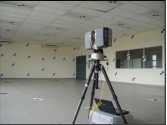
As shown in Figure 8, a self-calibration target field has been established in a laboratory with dimensions 15.5m x 9m x 3m. The 138 black and white targets were distributed on the four walls and ceiling based on conditions stated by Lichti [9].
Seven scan stations were used to observe the targets. As shown in Figure 9, five scan stations were located at the each corner and centre of the room. The other two were positioned close to the two corners with the scanner orientation manually rotated 90° from scanner orientation at the same corner. In all cases the height of the scanner was placed midway between the floor and the ceiling.
Fig. 8: Self-calibration for the Faro Photo 120 scanner.
In this experiment, the scan resolution was set to the 1/4 setting which is equivalent to the medium resolution. Higher resolution scans were not captured due to the longer time required to complete the scanning. Furthermore, medium resolution also was sufficient for Faroscene software to extract all targets except for those which have high incidence angle.
[image:5.595.298.540.111.250.2]After the scanning and target measurement processes were completed, a bundle adjustment was performed with precision settings based on the manufacturer’s specification, which were 2mm for distance and 0.009º for both angle measurements. After two iterations, the bundle adjustment process converged.
Fig. 9: Scanner locations during self-calibration.
5. Self-Calibration Results
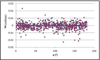
[image:5.595.83.254.350.478.2]In contrast with the hybrid scanner, the residual patterns of a panoramic scanner bundle adjustment can be used to detect the systematic error trends. As a result, other than statistical analysis, observation residual patterns are also used in this analysis. After performing the bundle adjustment process without any calibration parameters, residual patterns were plotted as a function of the adjusted observations as shown in Figures 10, 11 and 12.
Fig. 10: Range residuals as a function of adjusted range for the adjustment without calibration parameters.
[image:5.595.315.523.408.588.2]Fig. 12: Vertical angle residuals as a function of adjusted horizontal angles for the adjustment without calibration parameters.
Based on the sample of residual patterns shown in Figure 7, all significant systematic errors were investigated using the graphs from Figures 10 to 12. There are no systematic errors exhibited in both horizontal and vertical angles observations except for the range. The residual pattern graph has obviously demonstrated the trend of inclining line. Further analysis has been performed by running the bundle adjustment again using the calibration parameters. Results of the calibration parameters are shown in Table 1.
Table 1: Calibration parameters and their standard deviation
Table 2 presents the RMS of residuals for each observable group for the cases without and with the self-calibration. The results of RMS have shows the improvement in accuracy for up to 27% by implementing self-calibration procedure.
Table 2: RMS of residuals from the adjustments without and with self-calibration.
In order to have a high accuracy solution regarding the significant of the estimated systematic error models, statistical tests were performed. All calibration parameters were tested to investigate their significant. The hypotheses were set as follows:
H0 : The parameter is not significant.
HA : The parameter is significant.
Using 95% confidence level, the results of the test are shown in Table 3.
Table 3: Significant test for calibration parameters
Results from Table 3 above show that null hypothesis was rejected for all parameters. This indicates that those parameters are significant to the scanner observations. Even though the graphs of residual pattern above (Figure 10, 11 and 12) illustrated that only constant error was present in the observation, but mathematically all of error models are significant. As a conclusion, to ensure that the calibrated scanner (Faro Photon 120) gives accurate measurement, all point clouds are needed to be refined by applying all four systematic error models of a0, b0, b1 and
c0.
6. Conclusion
A self-calibration of the Faro Photon has been conducted over a dense 3D target field. The adjustment results were evaluated using graphs, which were based on residual pattern graph and mathematically utilising statistical analysis procedures. The differences between the RMS of residuals for adjustment with and without calibration parameters show an improvement up to 27%. Using the (t-test), the significant test was performed and the results show that all calibration parameters are statistically significant.
Acknowledgments
Authors would like to acknowledge the UiTM for the financial support for my PhD study. Special thanks goes to the Photogrammetry & Laser Scanning Research Group, INFOCOMM Research Alliance, UTM for the facility support in this project.
References
[1] Raja, V. and Fernandes, K.J. (2008). Reverse Engineering: An Industrial Perspective. Springer-Verlag London Limited 2008.
[image:6.595.308.538.112.235.2][3] Schulz, T. (2007). Calibration of Terrestrial Laser Scanner for Engineering Geodesy. A Dissertation submitted for the degree of Doctor of Scinces, Technical University of Berlin.
[4] Abdul, W. I. and Halim, S. (2001). Pelarasan Ukur. Kuala Lumpur: Dewan Bahasa dan Pustaka.
[5] Staiger, R. (2003). Terrestrial Laser Scanning: Technology, Systems and Applications. Second FIG Regional Conference, Marrakech, Morocco.
[6] Reshetyuk, Y. (2009). Self-Calibration and Direct Georeferencing in Terrestrial Laser Scanning. Doctoral Thesis in Infrastructure, Royal Institute of Technology (KTH), Stockholm, Sweden.
[7] Böhler, W., Bordas, V. M. and Marbs, A. (2003). Investigating Laser Scanner Accuracy. The International Archives of the Photogrammetry, Remote Sensing and Spatial Information Sciences, Vol. XXXIV (Part 5/C 15), pp. 696-701.
[8] Gordon, S., Davies, N., Keighley, D., Lichti, D. and Franke, J. (2005). A Rigorous Rangefinder Calibration Method for Terrestrial Laser Scanners. Journal of Spatial Science, Vol. 50:2, 91-96.
[9] Lichti, D. D. (2007). Error Modelling, Calibration and Analysis of an AM-CW Terrestrial Laser Scanner System. ISPRS Journal of Photogrammetry & Remote Sensing 61 (2007) 307-324.
[10] Brian, F., Catherine, L. C. and Robert, R. (2004). Investigation on Laser Scanners. IWAA2004, CERN, Geneva.
[11] Kersten, T. and Mechelke, K. (2008). Geometric Accuracy Investigation of the Latest Terrestrial Laser Scanning System. FIG Working Week 2008, Stockholm, Sweden.
[12] Luhmann, T., Robson, S., Kyle, S. and Harley, I. (2006). Close Photogrammetry: Principles, Methods and Applications. Whittles Publishing, Dunbeath Mains Cottages, Dunbeath, Scoland, UK.
[13] Lichti, D. D. (2010). A Review of Geometric Models and Self-Calibration Methods for Terrestrial Laser Scanner. Bol. Ciȇnc. Geod., sec. Artigos, Curitiba (2010) 3-19.
[14] Lichti, D.D. and Licht, M. G. (2006). Experiences with Terrestrial Laser Scanner Modelling and Accuracy Assessment. IAPRS Volume XXXVI, Part 5, Dresden.
[15] Lichti, D. D., Chow, J. and Lahamy, H. (2011). Parameter De-Correlation and Model-Identification in Hybrid-Style Terrestrial Laser Scanner Self-Calibration. ISPRS Journal of Photogrammetry and Remote Sensing 66 (2011) 317-326.
[16] Schneider, D. (2009). Calibration of Riegl LMS-Z420i based on a Multi-Station Adjustment and a Geometric Model with Additional Parameters. The International Archives of the Photogrammetry, Remote Sensing and Spatial Information Sciences, 38 (Part 3/W8)(2009) 177-182.
Mohd Azwan Abbas is currently PhD student at Department of
Geomatic Engineering, Universiti Teknologi Malaysia. He received the B.Sc. (2004) And M.Sc. (2006) in Geomatic Engineering from Universiti Teknologi Malaysia. His current interests include the calibration and 3D modeling using terrestrial laser scanner.
Halim Setan is a Professor at Department of Geomatic
Engineering, Universiti Teknologi Malaysia. He received M.Sc. (1988) in Geodetic Science from The Ohio State University, Columbus, USA and Ph.D. (1995) in Engineering Surveying from The City University, London, England. His current interests include the use of optical and range sensors for 3D reconstruction.
Zulkepli Majid is a Senior Lecturer at Department of Geomatic
Engineering, Universiti Teknologi Malaysia. He received the M.Sc (1998), B.Sc. (2004) And Ph.D. (2006) in geomatic engineering from Universiti Teknologi Malaysia. His current interests include the use of optical and range sensors for 3D reconstruction.
Albert K. Chong is a Senior Lecturer at Department of Geomatic
Engineering, University of Southern Queensland, Australia. He received the Ph.D. (1986) from University of Washington. His primary research focus is on the use of optical and range imagery for automated 3D object reconstruction.
Lau Chong Luh is currently PhD student at Department of
Geomatic Engineering, Universiti Teknologi Malaysia. He received the B.Sc. (2012) in Geomatic Engineering from Universiti Teknologi Malaysia. His current interests include the use of terrestrial laser scanner for 3D topography.
Mohd Farid Mohd Ariff is a Senior Lecturer at Department of
Geomatic Engineering, Universiti Teknologi Malaysia. He received the M.Sc (2005), B.Sc. (2002) And Ph.D. (2012) in geomatic engineering from Universiti Teknologi Malaysia. His current interests include the calibration and 3D reconstruction using photogrammetry technique.
Khairulnizam M. Idris is a Senior Lecturer at Department of
![Fig. 2: Beam deflection units used in TLSs [6].](https://thumb-us.123doks.com/thumbv2/123dok_us/152448.29592/2.595.46.285.569.701/fig-beam-deflection-units-used-tlss.webp)