IAF-97-A.5.08
Numerical Solutions for Lunar Orbits
M. Vasile and A.Ercoli Finzi
Dipartimento di Ingegneria Aerospaziale
Politecnico di Milano
Via Golgi 40 - 20133 Milano -Italy
48th International Astronautical Congress
October 6-10, 1997/Turin, Italy
NUMERICAL SOLUTIONS FOR LUNAR ORBITS
A.E.Finzi* and M.Vasile† Dipartimento di Ingegneria Aerospaziale
Politecnico di Milano Via Golgi 40 - 20133 Milano - ITALY
Abstract
Starting from a variational formulation based on Hamilton’s Principle, the paper exploits the finite element technique in the time domain in order to solve orbital dynamic problems characterised by constrained boundary value rather than initial value problems. The solution is obtained assembling a suitable number of finite elements inside the time interval of interest, imposing the desired constraints, and solving the resultant set of non-linear algebraic equations by means of Newton-Raphson method. In particular, in this work this general solution strategy is applied to periodic orbits determination. The effectiveness of the approach in finding periodic orbits in the unhomogeneous gravity field of the Moon is assessed by means of relevant examples, and the results are compared with those obtained by standard time marching techniques as well as with analytical results.
Introduction
The European programme for the exploration and scientific utilisation of the Moon proposes the injection of a probe into a low polar orbit. This class of missions being characterised by the strongly unhomogeneous lunar gravity field, the resulting perturbations could lead to rapid orbital decay and jeopardise the proper functioning of the equipment. Suitable methods and analysis tools to reliably and effectively address the problem of mission design become then of primary importance.
For most applications concerning Earth orbital dynamics, only the first term of the potential field are significant.Quite differently, a rather large number of terms must be taken into account in the Moon case and this makes the expression of the perturbing function complicate and the equations of motion strongly non-linear.
* Full Professor † Graduate Student
Copyright © 1997 by A.E.Finzi, M.Vasile. Published by the American Institute of Aeronautics and
Astronautics, Inc. with permission. Released to IAF/IAA/AIAA to publish in all forms.
The integration is therefore more difficult, a general solution to the problem in closed form cannot be obtained and a numerical integration is actually necessary.
Most of the numerical approaches proposed in the literature1 consider celestial mechanics problems as initial value problems for non-linear Ordinary Differential Equations (ODEs). By this approach very complex expressions of the gravitational potential and highly sophisticated models of non-conservative forces acting on the system can be afforded, however, the validity of these methods is limited by the initial conditions and period, selected for the integration.
In this paper, a novel methodology trying to remove these two limits is presented being many interesting problems in mission design indeed constrained boundary value (rather than initial value) problems for ODEs. A typical example are periodic orbits, which periodicity constraint can be considered as a boundary (initial and final time) condition on the state of the system. Other typical examples are orbital transfers and the related trajectory moves from one orbit to another, usually satisfying some optimality criterion. The use of the method of finite elements in time (FET) for the solution of constrained or un-constrained boundary value problems for orbital dynamics is here proposed. Instead of usual propagation, selecting a particular solution through the initial conditions and studying its evolution in time, a different philosophy is adopted, selecting a particular characteristic forced as a constraint. Then we look for solutions satisfying the condition imposed. The numerical solution is obtained discretising the time domain through the assembly of a suitable number of finite elements of appropriate order, and then imposing the relevant conditions.
unhomogeneous gravity field, neglecting optimality or other constraint conditions.
To this aim a model of the perturbing function, expressed in terms of spherical harmonics and orbital parameters and the equations of orbital dynamics in Poincarè parameters and Cartesian coordinates are presented. After that frozen and periodic orbits are briefly discussed and the method of Finite and Spectral Elements in Time introduced . Then the weak form of the problem according to Hamilton’s Principle is formulated and results obtained in a number of representative numerical simulations are presented.
The Moon Gravity Filed
The potential of the lunar gravity field given as expansion into spherical harmonics is a sum of the potential of a sphere and the perturbation accounting for all the deviations of a real body from a sphere4:
U r
r R
M
( , , )
(1)
R r
r
R
r P C m S m
M l
M l
lm m
l
lm lm
( , , )
( ) cos( ) )
2 0
[image:3.595.54.293.360.686.2]sin sin(
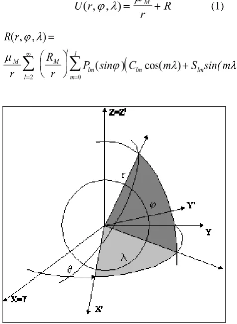
Figure 1. Spherical coordinates in a selenocentric reference frame: (X’,Y’,Z’) body fixed, (X,Y,Z) inertial.
The perturbing function can be expressed as a function of the usual keplerian orbital elements (a,e,I,,,M) and expanded as follows:
(2)
R a e i M
a
R
a
F i
G e S
M
M M
l
m l
lmp
q lpq lmpq
p l
l
( , , , , , )
( )
( )
( , , , )
0 0 2
(3)
S M
C l p q M l p m
S l p q M l p m l m
S l p q M l p m
C l p q M l p m l m
lmpq
lm lm lm lm
( , , , )
cos(( ) ( ) ( ))
(( ) ( ) ( ))
cos(( ) ( ) ( ))
(( ) ( ) ( ))
2 2
2 2
2 2
2 2
sin - even
sin - odd
where is the phase of the lunar rotation (see Figure 1), namely the angle between some body fixed direction along the equator (X’) and some inertial direction along the equator (X).
In (3) terms with l-2p+q0 (i.e., those containing the mean anomaly M) are very short periodic terms, those with l-2p+q=0 but m0 (i.e. those containing m) are medium periodic terms while those with both l-2p+q=0 and m=0 are long periodic terms.
Equations of Perturbed Motion
To integrate the Hamilton system that governs the perturbed orbital motion the problem in a canonical set of coordinates must be formulated.
As stated in the introduction most of the future lunar missions involve low polar orbiters. For this class of missions eccentricities must be small to avoid hard landing at periselenium. Low eccentricities, in turn, require non singular variables for e=0. Therefore we use two non-singular set of coordinate for solutions computations: Cartesian coordinates and Poincarè parameters.
Medium and long period terms (with Poicarrè parameters) are integrated and increased by short period effects the correction being performed in Cartesian coordinates. After the integration process we transform both Poicarrè parameters and Cartesian coordinate into the commonly used set of semiequinotial elements5:
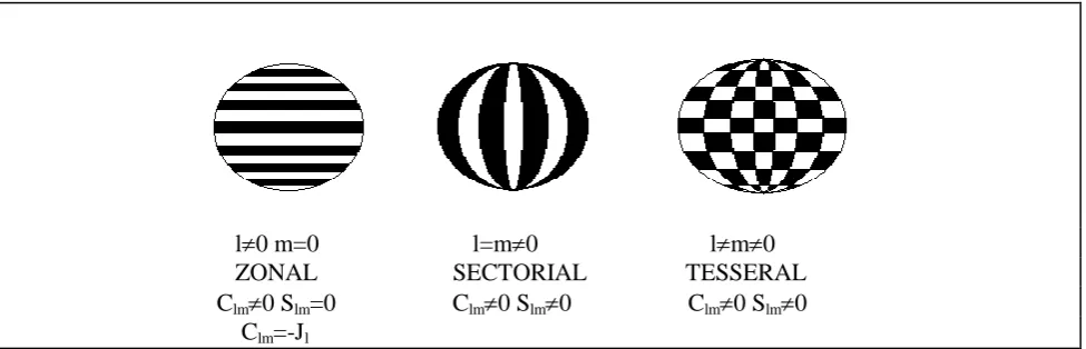
l0 m=0 l=m0 lm0 ZONAL SECTORIAL TESSERAL Clm0 Slm=0 Clm0 Slm0 Clm0 Slm0
Clm=-Jl
Figure 2. Geometrical interpretation of the harmonic coefficients. White areas represent elevations above and black areas represent depression with respect to the mean spherical surface of the body.
Poincarè Non-singular Canonical Parameters Formulation
In order to study medium and long period perturbations classical Keplerian parameters are transformed into a suitable canonical set of variables that are non-singular for e=0.
The coordinate system used (introduced by Poincarè3 ) is:
L a
E L e
H L e i
M L e
2 1 1
1
2 1 1
2 2
2
( )
cos
( ) cos
sin
(5)
the perturbation function written in the new variables set being:
R L E H
L
R
L
F
L E H
G
L E
S
L E
M M l l m l lmp p l l
q lpq lmpq
( , , , , , )
( , , , )
( , , )
( , , , , , )
2 2 2 0 0 2x
x
( 6)
and the Hamilton function:
( , , , , , ; ) ( , , , , , )
L E H
L R L E H
M 2 2 2
( 7)
Removing very short period perturbation, characterised by the terms with l-2p+q=0, by
means of an averaging process over an orbital period, the perturbing function reduces to:
( 8 )
R L E H
L R L
F L E H G L E S E
M l M l l m l p l
lmp lp l p lmp l p
( , , , , , ) ( , , , ) ( )( , , ) ( )( , , ; )
2 2 2 2 00 2 2
S E
C l p E m
S l p E m m even
S l p E m
C l p E m m odd
lmp l p
lm lm lm lm
( )( , , , )
cos(( ) a tan( / ) ( )) (( ) a tan( / ) ( )) cos(( ) a tan( / ) ( ))
(( ) a tan( / ) ( ))
2 2 2 2 2
sin l
-sin l
( 9 )
Notice that the variable L does not play any role because the force function does not depend on the fast variable , therefore the dynamics of medium and long period perturbations is described by four equations:
dE
dt
dH
dt
d
dt
E
d
dt
H
( 10 )
Cartesian Coordinates Formulation
As mentioned before short period perturbation are integrated in Cartesian coordinate. The perturbing function in this set of coordinates is:
( 11 )
R r R r P z rC m y
x m S m
y x m M M lm lm l l m l lm ( ) =
a + sin a
=2 + = r
0 [image:4.595.56.544.76.233.2]and Hamilton’s function:
1
2
p p
*
U
( )
q
( 12 ) where we callq
=
r
p
d
r
dt
( 13 )U
r R
( )q ( )q ( 14 )
Thus the Hamilton’s system holds:
d
dt
U
d
dt
p
q
q
p
(
15)
The Frozen Solutions
Previous to the following analysis of periodic solutions we search for frozen solutions of the system (10), namely solutions that do not present any long period variations of eccentricity, argument of the periapsis and inclination.
Thus we remove medium period perturbation from (8), e.g. terms with m0. Therefore the perturbing function contains only the so called ‘zonal’ harmonics of the gravity field (Figure 2).
In this averaged force field the component of the angular momentum along the lunar polar axis is an integral of motion:
dH
dt
0
H
Ma
1
e
i
t
2
(
) cos
cos .
(16) thus a separate equation of motion for i is not needed and we can reduce to:dE
dt
d
dt
E
= 0
= 0
(
17)
The first one is satisfied for 13 =/2, while the second one can be solved numerically for E. Using the values of E and is then possible to compute the value for e by the following equation:
e
L
L
E
E
1
2
4
2 2 2 2
(
)(
)
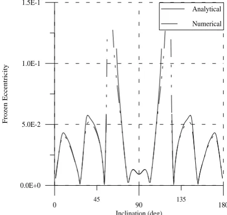
( 18) Frozen values of e and as a function of the inclination are plotted in Figure 4 and compared with analytical ones2. The two solutions are ingood agreement for all the inclination angles apart from critical inclinations where the eccentricity dramatically grows and linearised analytical theory are not enough accurate. It should be noted that generally equation (17) doesn’t have only one solution. However solutions corresponding to high eccentricity values are not generally suitable for a low altitude orbiter. In fact13 this solution become practicable for altitude above 3000 km.
In order to determine the minimum number of harmonics degree giving a reliable frozen solution in Figure 3 frozen eccentricities as a function of zonal harmonics degree, for an inclination of 90 degrees and an altitude of 100 km, are plotted and the plot shows that 21 harmonics at least must be considered.
10 30 50
0 20 40 60
Zonal Harmonics Number
1.0E-2 3.0E-2 5.0E-2 7.0E-2 9.0E-2
0.0E+0 2.0E-2 4.0E-2 6.0E-2 8.0E-2
F
ro
z
e
n
E
c
c
e
n
tr
ic
it
[image:5.595.328.545.289.495.2]y
Figure 3. Frozen eccentricity as a function of the harmonic degree, a=1838 km, i=90°.
45 135
0 90 180
Inclination (deg) 0.0E+0
5.0E-2 1.0E-1 1.5E-1
F
ro
z
e
n
E
c
c
e
n
tr
ic
it
y
Analytical Numerical
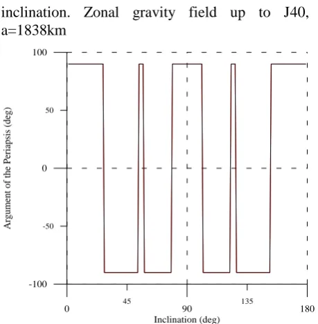
[image:5.595.315.544.540.757.2]inclination. Zonal gravity field up to J40, a=1838km
45 135
0 90 180
Inclination (deg)
-50 50
-100 0 100
A
rg
u
m
en
t
o
f
th
e
P
er
ia
p
si
s
(d
eg
)
Figure 5. Frozen argument of the periapsis as a function of inclination. Zonal gravity field up to J40, a=1838 km.
The SET Approach
Hamilton’s Principle implementation in numerical approaches for dynamics dates back to more than 25 years ago7,8 . A complete review of the literature devoted to the finite element method in the time domain is beyond the scopes of this work, however it seams important to stress that the method has been successfully applied to a large number of problems in computational mechanics, spacing from rigid body dynamics to structural mechanics, wave propagation, fluid dynamics and optimal control9,10.
In this paper we propose a slightly different approach using, instead of FET, Spectral Elements in Time (SET) a high-order finite element technique that combines the geometric flexibility of finite elements with the high accuracy of spectral methods. The method, pioneered in the mid 1980's by Anthony Patera11 at MIT for fluid dynamics problems, is here applied to the integration of ODEs in the time domain being spectral elements in time more accurate and efficient in finding the solution for our problems involving less memory space and less computational cost.
Both FET and Spectral Elements methods offer some interesting features that make them attractive in automated numerical procedures:
Using a time assembly process, they allow the solution of general boundary-value problems. Besides the computation of the system response, this technique provides at
a negligible extra computing cost an approximation of the transition matrix that allows to perform a linearised stability analysis of the solution9.
Through the use of spectral basis for shape functions, high order methods can be constructed, therefore allowing the development of automated p and hp
adaptive procedures.
The variational framework is an ideal context for developing constrained formulations for mechanics10, leading to schemes characterised by robust numerical behaviour. As stated in the Introduction, the ability to impose constraint conditions of different nature on the orbital boundary value problem, is a key ingredient of a general mission design tool.
Both the Lagrangian (single-field) and the Hamiltonian (mixed two-field) formulations of the FET method can be developed. Since the late is usually associated with superior numerical properties10, in the following we restrict our discussion to the mixed two-field case.
Solution of Orbital Problems by the SET
In order to apply the SET method in mixed two-field form to the problems of orbital dynamics we utilise a set of generalised coordinates q, momenta p, non-conservative generalised forces Q and Hamiltonian function
=(q,p):
p
q
Q
q
p
( 19 )In conservative problems, as is the case, non-conservative forces Q disappear.
Equations (15) are supplemented by the boundary conditions:
p p p p
q q q q
( ) ( )
( ) ( )
t t
t t
i ib f bf
i ib f bf
( 20 )
where (.)b denotes boundary values and ti and tf
[image:6.595.56.286.69.303.2]are prescribed, while the others are to be regarded as additional unknowns.
Equations (19) and (20) can be cast in a weighted residual form, which after integration by parts, yields Hamilton’s Law in mixed two-field form: ( 21)
t t t t i f i f dt b b
p q q p
q q p p
p q q p
* * * * * *
The variational principle (21) is the weak form of the differential problem given by (19) and (20). This synchronous formulation provides the base for the development of the SET methods for general boundary problems, where the integration time domain is known a priori. However in many problems of orbital mechanics time can be regarded as an additional unknown. In this case, the asynchronous version of Hamilton’s Law can be derived and used for developing parametric versions of the SET method.
Now let the time domain D(ti,tf) be decomposed into N finite time elements:
D Nj D t t
j i i
1 ( , 1) ( 22) The parametric approximations of the trial functions (q,p) and test functions (q,p) are developed within the space of the polynomials of order k-1 and k respectively:
q
q
p
p
q
q
p
p
s k s s s k s s s k s s s k s sf t
f t
g t
g t
1 1 1 1 1 1
( )
( )
( )
( )
( 23)where the functions f and g are defined as follow:
f
P
D
g
P
D
k k j j
1(
)
(
)
( 24) and the quantities qs and ps are internal nodevalues.
In a more general way we could decompose de domain D as a union of smooth images of the reference time interval [-1,1] where we define a reference parameter :
2 1 2 2
1 1 2 t t t t t t t i i i i / /
( 25 ) The basis functions f and g can be constructed by using Lagrangian interpolants associated with the internal Gauss-Lobatto node12. Thus if i
k
i=1 are the set of Gauss-Lobatto
points on the reference interval [-1,1], fi() will be the Lagrangian interpolating polynomial vanishing at all the Gauss-Lobatto node except at
i where it equals one.
Each integral of the continuous form (21) is then replaced by a Gauss quadrature sum:
i n
i i i
i i
i n
i i i
i i
p
q
q
q
t
q
p
p
p
t
1 12
2
( )
( )
( )
( )
( )
( )
( )
( )
( 26 )where i is the weight associated with i.
By the discrete form (26) two distinct procedures can be derived:
An implicit step-by-step self-starting integration obtained for initial value problems
An assembled process developed for boundary value problems, obtained by matching the final boundary state of each element with the initial state of the subsequent element.
Both the approach are taken into account in this effort, and the resulting non-linear algebraic equations can be linearised with the help of Newton-Raphson method to yield:
) ( ) ( )
(e u e Re
J ( 27 ) where J(e) is the elemental tangent matrix, R(e)
the elemental residual vector, u(e)=(p,q)(e) are
increments to nodal momenta and nodal coordinates, while the subscript (.)(e) refers to
elemental quantities. The global matrix formulation can then be obtained through the standard finite element assembly process performed on the corresponding elemental matrices:
R
u
J ( 28 ) The Periodic Constraint
As previously stated given the importance of periodic orbits in several celestial mechanics problems, we look for solutions that satisfy the constraint of periodicity. This constraint requires that the final state vector (qbf,p
b
initial state vector (qbi,pbi). It could be handled as
a general homogeneous boundary-conditions problem for the differential system (19), by the equations:
q
q
p
p
f b
i b
f b
i b
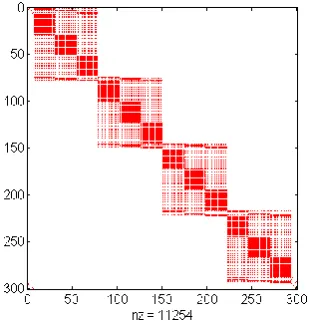
( 29 )The tangent matrix J is generally a sparse structure matrix as shown in Figure 6. For the solution of the linear system (28) a preconditioned GMRS sparse matrix solver with CRS (Compressed Row Format) storage of the matrix is used.
Figure 6. Assembled tangent matrix for a 4 elements system in Cartesian coordinates and for a tesseral gravity field.
Stability Analysis of Periodic Orbits
The stability of any periodic solution got from the assembled process can now be afforded by the linearised stability analysis proposed in 9.Starting from:
A X K B i ( 30 ) where the vector X is defined as follows:
X
X
i,
B
f T ( 31 ) the two vectors Bi and Bf are perturbationsrespectively of the initial and final boundary values while Xi are the variations of the
internal nodes, and remembering that matrixes A and K can be easily obtained by a pertition of the matrix J:
J
K
A
J
J
i f
( 32) inverting the matrix A (which is an upper triangular matrix) we get:
X
i,
B
f
T
A K B
1
i( 33) Finally the transition matrix T between the initial and the final state can be derived:
Bf T B i ( 34 ) As in the Floquet theory, we search for recurring solutions of equation (30) such as
Bf
Bi ( 35 ) which leads to an eigenvalue problem that can be directly solved in the range of the highest of interest. Eigenvalues and the corresponding eigenvectors are in general pairs of complex conjugate ones. Moreover, an approximation of each complex eigensolution at nodal points can be given by the solution of equation (35), by using the corresponding eigenvalue and eigenvector9.When the interest is focused on limit stability, the sole eigenvalue analysis is required. In fact stability is provided by the condition 1 where is the modulus of the eigenvalue .
Numerical Simulations
To verify the effectiveness of the proposed methodology in the following some meaningful tests problems are presented for comparison with both analytical and numerical solutions. Being the method completely independent from the potential function, all the examples here presented refer to Lemoine’s gravity model5
GLGM-2.
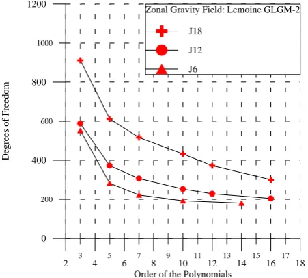
Accuracy Analysis
[image:8.595.104.259.267.428.2]3 5 7 9 11 13 15 17
2 4 6 8 10 12 14 16 18
Order of the Polynomials
200 600 1000
0 400 800 1200
D
eg
re
es
o
f
F
re
ed
o
m
Zonal Gravity Field: Lemoine GLGM-2
J18
J12
J6
Figure 7.
Degrees of Freedom to achieve a desired accuracy as function of zonal degrees.Periodic Solution in a Zonal Gravity Field The ability to identify periodic solutions in a zonal gravity field taking into account both long and short period perturbations is tested. For this particular problem the only possible periodic solution are orbits with an inclination of 90° degrees whole within the initial orbital plane. Thus we relax the periodicity constrained (24) forcing the initial state vector to be exactly on one of the pole:
x
x
x
y
y
y
z
z
z
z
i b
f b
i b
i b
f b
i b
f b
i b
f b
i b
0
0
;
;
;
( 36 )
The force field depends on the positions, thus the three constraints on the è position components and the one on the z component of the velocity, which provides the periodicity on the versus of the velocity, guarantee the complete periodicity of the final solution.
In Figure 8 we present the periodic solution obtained by this innovative approach. In order to validate the results, we use the value of the solution at time ti=0 as an initial
state and we integrate using a 7-8th order Runge-Kutta-Fehlberg (RK) method with adaptive time stepping. The result obtained with the Runge-Kutta integration is presented as a solid line in Figure 8.
The FET and the Runge-Kutta solution appear to be in very good agreement. The
solution of this problem should be a frozen orbit, since periodic orbits are certainly frozen because they do not present any long period variations. Thus for further validation of the new methodology, the mean eccentricity and the mean argument of the periapsis are computed and compared to ones computed in
frozen analysis. By calculation frozen solution
gives e=0.00909 and =90, while the SET gives e=0.009089 and =90.0000007.
These values prove that a periodic frozen orbit was found as proved by figure 8 showing the solution in semi-equinotial coordinates obtained with 10 elements and polynomials of the 11th order: in the plane h-k the solution is a closed trajectory around the mean values for e and and moves clockwise along the curve.
-1.0E-4 1.0E-4
-2.0E-4 0.0E+0 2.0E-4 k=e*cos(omega)
8.6E-3 9.0E-3 9.4E-3
8.8E-3 9.2E-3 9.6E-3
h
=
e
*
si
n
(o
m
e
g
a
)
FET RK
Figure 8. Periodic solution, h-k plane: 40x0 zonal gravity model. Integration period 7070.93s.
2000.0 6000.0
0.0 4000.0 8000.0 Time (s)
1837.4 1837.8 1838.2
1837.2 1837.6 1838.0 1838.4
S
em
im
aj
o
r
ax
is
(
k
m
)
[image:9.595.57.283.72.275.2]FET RK
[image:9.595.318.530.293.489.2] [image:9.595.314.534.537.741.2]We can underline also that, as can be noticed from Figure 9, the mean semi-major axis found by the SET method is smaller then the unperturbed one. In fact perturbations due to zonal harmonics increase the mean revolution period for polar orbits1. Therefore closed orbits with a period equal to the reference one require shorter mean semi-major axis according to its relation with the mean motion.
Periodic Solutions in a Tesseral Gravity Field We are now searching for periodic solutions in a tesseral gravity field.
Being the rotation period of the moon of 29.3216 sidereal days. This means that a satellite sees the same gravity field every 29.3216 days. Thus in a tesseral gravity field containing terms characterised by the index m0 that take care of this rotational motion, as was shown in equation (3), a periodic solution could be found integrating over a period of at least 29.3216 days.
The wide spectrum of frequencies introduced by the perturbing function and the wide integration period lead to a large number of spectral elements necessary to follow correctly the dynamics of the problem. Thus at first the dynamics of mean parameters is solved and then short period perturbations added.
Mean Motion Analysis
By remotion of very short period perturbations the dynamics of periodic orbits can be studied with a relative low number of elements.
The first test afforded is a periodic mean orbit in a 6x6 gravity field. We use 22 spectral elements with polynomial of order 7 and we force the periodicity constraints:
E E
H H
ib bf fb
i b
f b
;
ib
;( 37 )
A further periodicity constraint could be forced on the anomaly of the ascending node for polar orbits only:
ib
f b
;
( 38 ) In fact for these orbits there is no secular motion of the ascending node. For different inclinations, orbits can not be closed and the constraint (38) becomes:
ib
f b
;
( 39 ) Where the term takes care of the precession motion.The solution for a polar orbit is shown in figure 10. Now short period perturbations are added and starting from the periselenium at t=0 (=0), we propagate over 58.6422 days using the SET time marching algorithm with a fixed time step of 835.2s. The solution is represented in figure 11 ( h and k parameters) and in figure 12 (i
and parameters).
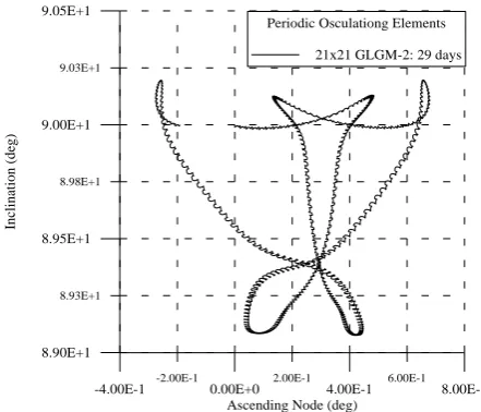
As second test we study a 21x21 gravity field using 50 elements with polynomials of 10th order and the results for mean elements are plotted in figure 12. Then we propagate short period perturbations using fixed time step of 707.9 s and we plot results for mean elements in figure 13 and for osculating elements in figures 14 and 15. By comparison the frozen solution with the mean elements values found with periodic solutions, reported in table 1 and 2, we conclude that also in these two cases we found a periodic frozen orbit.
It should be noted that both these solutions are unstable: a small variation in the mean value of the inclination giving a secular term in the dynamics of the ascending node (precession of the ascending node) and brakes the periodicity of the solution.
This instability is however very weak as it is confirmed by the stability analysis which gives the highest eigenvalues close to one for both the solutions computed: max =1.0006.
The effects of this instability are well represented in figure 12 and 15 where the precession of the ascending node, due to perturbations given by short period terms, is evident. The difference between the initial and final value of the ascending node is however quite small for both the examples.
Table 1. Comparison between frozen and periodic solution for a 6x6 gravity field: mean values.
e
Periodic 3.9826e-2 -90.0001
Frozen 3.98264e-2 -90
Table 2. Comparison between frozen and periodic solution for a 21x21 gravity field: mean values.
e
Periodic 9.2226e-3 90.00016
-6.00E-3 -2.00E-3 2.00E-3
-4.00E-3 0.00E+0 4.00E-3
k=e*cos(w) -4.25E-2
-3.75E-2
-4.50E-2 -4.00E-2 -3.50E-2
h
=
e*
si
n
(w
)
[image:11.595.318.537.69.255.2]Periodic Mean Elements 6x6 GLGM-2: 29 days
Figure 10. Mean h-k plane, periodic solution, 6x6 model, a=1838.96364 km, i=90°.
-2.50E-3 2.50E-3
-5.00E-3 0.00E+0 5.00E-3
k=e*cos(w)
-4.25E-2 -3.75E-2
-4.50E-2 -4.00E-2 -3.50E-2
h
=
e*
si
n
(w
)
Periodic Osculating 6x6 GLGM-2: 58 days
Figure 11. Osculating h-k plane, quasi-periodic solution, 6x6 model, propagation over 58 days .
-57.00 -56.60 -56.20 -55.80
-57.20 -56.80 -56.40 -56.00
Ascending Node (deg)
89.40 89.80 90.20 90.60
89.60 90.00 90.40 90.80
In
c
li
n
a
ti
o
n
(
d
e
g
)
Periodic Osculating 6x6 GLGM-2: 58 days
Figure 12. Osculating I- plane, quasi-periodic solution, 6x6 model, propagation over 58 days
-6.00E-3 -2.00E-3 2.00E-3 6.00E-3
-8.00E-3 -4.00E-3 0.00E+0 4.00E-3 8.00E-3 k=e*cos(omega)
3.00E-3 9.00E-3 1.50E-2
6.00E-3 1.20E-2 1.80E-2
h
=
e*
si
n
(o
m
eg
a)
Periodic Mean Elements 21x21 GLGM-2: 29 days
Figure 13. Mean h-k plane, periodic solution, 21x21 model.
-6.00E-3 -2.00E-3 2.00E-3 6.00E-3
-8.00E-3 -4.00E-3 0.00E+0 4.00E-3 8.00E-3 k=e*cos(omega)
3.00E-3 9.00E-3 1.50E-2
6.00E-3 1.20E-2 1.80E-2
h
=
e*
si
n
(o
m
eg
a)
Periodic Osculationg Elements 21x21 GLGM-2: 29 days
Figure 14. Osculating h-k plane, quasi-periodic solution, 21x21 model, propagation over 29 days.
-2.00E-1 2.00E-1 6.00E-1
-4.00E-1 0.00E+0 4.00E-1 8.00E-1 Ascending Node (deg)
8.93E+1 8.98E+1 9.03E+1
8.90E+1 8.95E+1 9.00E+1 9.05E+1
In
cl
in
at
io
n
(
d
eg
)
Periodic Osculationg Elements 21x21 GLGM-2: 29 days
[image:11.595.72.290.70.258.2] [image:11.595.57.278.294.485.2] [image:11.595.319.535.295.487.2] [image:11.595.63.273.538.734.2] [image:11.595.315.536.542.731.2]Final Remarks
In this paper a novel approach to the numerical solution of a certain class of orbital dynamic problems is presented. The inspiring idea of the method is the use of SET formulation for constrained boundary-value problems for non-linear ODEs. This method is expected to be a valid and reliable tool for the mission designer.
Even if the results achieved in this study are to be considered preliminary, however they provide evidence of the effectiveness of the new approach: in fact all the results obtained by the SET methodology are confirmed both by the analytical solutions and the usual numerical propagation.
This results open the way to a range of interesting future developments, aimed to enhancing the effectiveness of the method and at broadening its applicability to more complex problems among which the use of global optimisation methods is at present being studied.
References
[1] F.Sansò, R.Rummel, Theory of Satellite Geodesy and Gravity Field Determination,
Lecture Notes in Earth Sciences, Vol. 25, Springer-Verlag, 1988.
[2] S.Y. Park, J.L. Junkins, Orbital Mission Analysis for a Lunar Mapping Satellite. The Journal of the Astronautical Sciences, Vol.43, No.2, April-June 1995, pp.207-217. [3] A.Milani and Z.Knezevic, Selenocentric Proper Elements, A Tool for Lunar Satellite Mission Analysis, Consorzio Pisa Ricerche. Report No. 144506 of 19/12/1994, May 20, 1995.
[4] R.Floberghagen, R. Noomen, P.N.A.M. Visser, and G.D. Racca, Global Lunar Gravity Recovery from Satellite-to-Satellite Tracking, Planet. Space Sci. Vol. 44, No. 10, 1996, pp. 1081-1097.
[5] F.G.Lemoine, D.E.Smith and M.T.Zuber, A 70th Degree and Order Gravity Model for the Moon, P11A-9, EOS, Trans. American Geophys. Union, Vol. 75, No. 44, 1994. [6] D.Brouwer and G.M. Clemence, Methods
of Celestial Mechanics, Academic Press, Inc., NY, 1961.
[7] J.H.Argyris and D.W.Scharpf, Finite
Elements in Time and Space.
Aeronaut.J.Roy. Aeronaut.Soc.,Vol. 73, 1969, pp. 1041-1044.
[8] I.Fried, Finite-Element Analysis of Time-DependentPhenomena, AIAA Journal,Vol. 7, No. 6, June 1969, pp.1170-1173.
[9] M.Borri, Helicopter Rotor Dynamics by Finite Element Time Approximation. Comp.&Maths. with Appls., Vol. 12A, No.1, 1986, pp. 149-160.
[10] M.Borri and P.Mantegazza, Finite Time Element Approximation of Dynamics of Non-holonomic Systems, AMSE Congress, Williamsbury, Virginia, USA, August 1986.
[11] G.E. Karniadakis, E.T. Bullister and A.T. Patera, A spectral element method for solution of two- and three-dimensional time-dependent Navier-Stockes equations,
Proc. Europe-U.S. Conf. on Finite Element Methods for Nonlinear Problems, Springler-Verlag, p.803, 1985.
[12] L.F.Pavarino,Preconditioned Mixed Spectral Elements Methods for Elasticity and Stokes Problems. AMS(MOS) subject classifications.65f10