Mode choice with latent availability and consideration: Theory and a case study

This is a repository copy of Mode choice with latent availability and consideration: Theory and a case study.

White Rose Research Online URL for this paper: http://eprints.whiterose.ac.uk/118260/

Version: Accepted Version

Article:

Calastri, C, Hess, S orcid.org/0000-0002-3650-2518, Choudhury, C

orcid.org/0000-0002-8886-8976 et al. (2 more authors) (2019) Mode choice with latent availability and consideration: Theory and a case study. Transportation Research Part B: Methodological, 123. pp. 374-385. ISSN 0191-2615

https://doi.org/10.1016/j.trb.2017.06.016

© 2017 Elsevier Ltd. This manuscript version is made available under the CC-BY-NC-ND 4.0 license http://creativecommons.org/licenses/by-nc-nd/4.0/

[email protected] https://eprints.whiterose.ac.uk/ Reuse

This article is distributed under the terms of the Creative Commons Attribution-NonCommercial-NoDerivs (CC BY-NC-ND) licence. This licence only allows you to download this work and share it with others as long as you credit the authors, but you can’t change the article in any way or use it commercially. More

information and the full terms of the licence here: https://creativecommons.org/licenses/

Takedown

If you consider content in White Rose Research Online to be in breach of UK law, please notify us by

1

Mode choice with latent availability and consideration: theory and a

case study

Authors: Chiara Calastri*, Stephane Hess*, Charisma Choudhury*, Andrew Daly*, Lorenzo

Gabrielli~

* Institute for Transport Studies & Choice Modelling Centre, University of Leeds, UK

~ KDD Lab. - Istituto ISTI - Area della Ricerca CNR di Pisa, Italy

Abstract

Over the last two decades, passively collected data sources, like Global Positioning System (GPS) traces from data loggers and smartphones, have emerged as a very promising source for understanding travel behaviour. Most choice model applications in this context have made use of data collected specifically for choice modelling, which often has high costs associated with it. On the other hand, many other data sources exist in which respondents’ movements are tracked. These data sources have thus far been underexploited for choice modelling. Indeed, although some information on the chosen mode and basic socio-demographic data is collected in such surveys, they (as well as in fact also some purpose collected surveys) lack information on mode availability and consideration. This paper addresses the data challenges by estimating a mode choice model with probabilistic availability and consideration, using a secondary dataset consisting of ‘annotated’ GPS traces. Stated mode availability by part of the sample enabled the specification of an availability component, while the panel nature of the data and explicit incorporation of spatial and environmental factors enabled estimation of latent trip specific consideration sets. The research thus addresses an important behavioural issue (explicit modelling of availability and choice set) in addition to enriching the data for choice modelling purposes. The model produces reasonable results, including meaningful value of travel time (VTT) measures. Our findings further suggest that a better understanding of modes choices can be obtained by looking jointly at availability, consideration and choice.

1. Introduction

In recent years, there has been increasing interest in using ubiquitous data sources for behavioural modelling in different fields of research.

2

(usually minimal) input from the users, like correcting their passively collected trajectories or adding details about their trips.

In the context of transport and mobility, GPS data (collected via different devices, such as black boxes in cars, portable loggers or smartphones) have been used since the mid-90s.

Most of the existing research has focussed on improving GPS data quality using smoothing and map matching techniques (Quddus et al., 2007) and identifying trip details like departure time, trip purpose (e.g. Shen & Stopher, 2013; Schuessler & Axhausen, 2009; Chen et al., 2010; Stopher et al. 2008) and travel mode (e.g. Schuessler & Axhausen, 2009; Bohte & Maat, 2009; Chen et al., 2010; Tsui & Shalaby, 2006; Feng & Timmermans, 2015). Some research efforts also focused on the assessment of public transport infrastructures (Bullock, P. and Jiang, Q. 2003; Greaves et al. 2014); traffic flows and similar phenomena (Quiroga et al. 2002), analysis of individual travel behaviour patterns (Broach et al. 2012) and evaluation of policies (Stopher et al. 2009). Several studies have compared the quality of GPS data with phone and paper recall surveys and traditional travel diaries to find under-reporting in the latter (Casas & Arce, 1999; Murakami & Wagner, 1999; Kelly et al., 2013).

However, despite the better accuracy, lower costs, lower respondent burden and availability of multiple observations for the same traveller, the use of the GPS data in econometric models of travel behaviour has been primarily limited to models for route (e.g. Bierlaire et al. 2008; Bierlaire et al. 2010; Hess et al. 2015; Prato 2009; Broach et al. 2012; Dhakar & Srinivasan, 2014), destination (e.g. Huang & Levinson, 2015; Miyashita et al. 2008) and tour pattern (Iqbal et al. 2012) choice. The lack of attention paid to mode choice is believed to be mainly due to the lack of information about the attributes of the unchosen (and in some cases the chosen) alternative(s) and absence of information regarding the characteristics of the decision makers and their choice sets – this is quite different in a mode choice context from, for example, a route choice context.

A first research issue that this paper aims to address at least in part is thus how analysts can better accommodate mode availability and consideration when working with GPS data. Existing studies have suggested a number of different approaches to deal with consideration in choice models (Manski, 1977; Swait and Ben-Akiva, 1987; Cascetta and Papola, 2001; Cantillo and Ortúzar, 2005). We address this by proposing a latent class approach which treats mode availability and consideration in a probabilistic manner, with the former being at the person level and the latter at the trip level.

Applications using GPS data in travel behaviour modelling also generally rely on data collected specifically for that purpose. However, because of the relative ease of collecting these data, more and more businesses, research centres and public institutions have started to set up projects for diverse purposes that are different from travel behaviour modelling, such as detecting congestion flows or simply providing an accessible overview of mobility in a city or limited area by different visualisation techniques.

3

collected for purposes other than travel behaviour modelling, and the investigation of whether and how these sources can be used for our analyses is our second research question. In the context of such non-customised data, dealing with mode availability and consideration is even more complex. The development of methodologies and techniques able to overcome some of the challenges related to these data could be the key to accessing a valuable resource and gaining new insights into travel behaviour.

This paper attempts to address both of the above questions (use of data collected for non-modelling reasons, and accommodating unobserved mode availability and consideration) using a dataset from Italy consisting of ‘tagged’ GPS traces where the trips, passively recorded by a smartphone GPS application, were subsequently annotated by respondents with trip modes and purposes.

The remainder of this paper is organised as follows. The next section presents the data used in our study. This is followed in the third section by a presentation of the modelling approach adopted, while the fourth section details the empirical application and reports the estimation results. The last section concludes the paper with discussion of the insights gained through this modelling experiment and outlines potential future research directions.

2. Data

2.1 Data collection

The data used for the present research were collected by the Italian National Research Council in the context of the Tag My Day project, with the generic scope of gaining a better understanding of urban mobility and providing suggestions to policy makers to improve traffic problems, but without the explicit aim of travel behaviour modelling. The data collection took place in the city of Pisa (Italy) and surrounding areas between May and October 2014. Pisa is a medium sized city (approx. 91,000 permanent inhabitants, but also hosting approx. 51,000 students, most of whom are not residents) in the Tuscany region. The city is served by buses (there is no metro or light-rail service), and trains are only used for inter-city trips. There are 17 urban bus lines, of which 15 operate during the day (approximately 6 AM until 9 PM) and 2 during the night. At the time of the survey, a bike sharing system had recently been introduced, with 10 pick-up and drop-off stations. The city centre, as in most Italian cities, is very compact and walking and cycling are widely used modes especially among students, although car remains the main mode of transport for most residents.

4

successive readings also depends on the ability of the logger to connect to receive a signal from the satellites; in our data, the median gap between readings was 6 seconds, and the median spatial gap was 11 metres. This represents a high level of accuracy, going beyond the level of precision required for a mode choice application such as presented here.

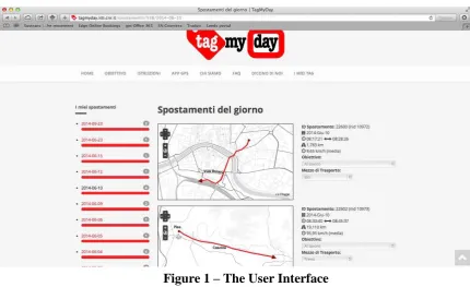
Recorded trajectories were displayed in users’ personal area of the Tag My Day website. Here, they could visualise each trip on a map, together with start and end time and average speed. Respondents were then asked to add information for each displayed trip in relation to travel mode and purpose. The “mode” dropdown menu listed 8 possible options: car, bicycle, walking, bus, train, taxi, boat, other. The “purpose” field included 12 categories: going to work, eating out, social activities (pub, visits to friends and family, gatherings), pick up-drop off, getting fuel, errands (bank, doctor, hairdresser), grocery shopping, other shopping, stop/mode change, study, leisure (sport, day trips, museums), going home. Two additional categories were provided to indicate problems with the recorded trip, one for incomplete trips due to app crash or low battery and one for wrong trajectory due to GPS errors.

Figure 1 represents a screenshot of the user interface: all the days for which trips have been recorded are displayed on the left hand side, while the selected day’s trips are each presented in detail, alongside a map.

Figure 1 – The User Interface

Participants were asked to use the app to record and annotate all their trips for at least one week, but they could keep using the system until the end of the survey period, if they wanted. This resulted in high variability in the number of trips recorded across people. As an incentive to take part in the project, people could accumulate “points” through greater engagement with the app/online portal, and these points entitled them to lottery tickets to win a number of prizes in the form of bicycles and iPads.

5

participants afterwards, collecting information on mode availabilities, job type and attitudes, and this was completed by 54 of the respondents.

2.2 Data cleaning and censoring

A number of distinct criteria were used in cleaning the data in preparation for the modelling work:

 A small number of taxi trips and inter-city trips by train were removed in order to focus on intra-urban mobility and limit the number of choice alternatives. Train trips were excluded because of their exclusively inter-urban nature, while taxi trips, although urban, were negligible in number. This implied that all the trips included in the dataset were by foot, bicycle, scooter, car or bus.

 The focus of our study is not on inferring mode choice but to understand actual observed mode choices. We therefore focus only on respondents who tag all their trips.

 In a few cases, participants reported trips by modes that they stated as unavailable to them and these trips were excluded.

 We also excluded trips that were annotated as having the purpose of getting fuel, technical stop (e.g. traffic lights, congestion) and those flagged by users as errors or incomplete trips. No mode choice would have taken place for those trips.

 Finally, in order to avoid an excessive impact by a few outliers on the coefficients, we only included trips shorter than 50km; this approach is also in line with the focus on urban mobility.

A further issue arises as a result of the data collection protocol, given the open-ended participation. In order to avoid people with an extremely high number of repetitive trips having excessive impact on our results, we decided to limit the heterogeneity in the number of trips. We excluded from our sample the people who reported fewer than 5 trips, and we limited the maximum number of trips per person to 200. Only a few reported a number of trips higher than this upper limit, and in these cases, the 200 trips to be used in the modelling were randomly selected. The final sample thus contained 5,149 trips, recorded by 102 participants, which included the 54 respondents who also completed the follow-up questionnaire. Males (70%), people with a highly level of education (50%) and young people (90% of the sample is younger than 45 years) are over-represented, probably because the survey was mainly advertised at the University and through social media.

6

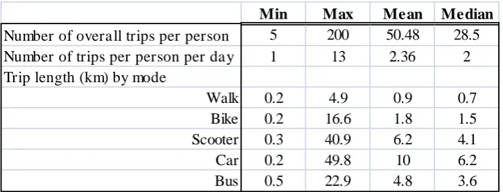
Table 1 and 2 report some characteristics of the trips recorded by people in the selected sample. While most people reported a low number of trips, with approximately 40% of the sample reporting fewer than 20 trips, Table 1 shows that, the high number for some leads to a median of 28.5. Some of this variation is of course a result of using the app over a shorter or longer period. On average, people reported 2.36 trips per day, a figure slightly lower than those achieved by some other GPS-based studies (Safi et al., 2015; Bohte and Maat, 2009; Stopher and Wargelin, 2010). Given the specific app usage protocol, a comparison is difficult, as most studies rely on devices which automatically detect when the user starts moving.

Table 1 – Number of trips per person and trip length by mode

Table 2 – Number of trips by purpose and mode

As expected, the longest trips were by car (just under 10 km on average), followed by scooter, bus, bicycle and walk, as shown in Table 1. Table 2 reports the number of trips by mode and purpose. The largest number of the trips (33%) are towards home and a vast majority of them are by car. Car is also observed to be the most frequent choice for other purposes, especially work and social. The sample contains a very low number of trips by bus, only 1% of the total.

2.3 Data enrichment

As mentioned above, basic socio-demographic information such as gender, age and level of education were collected upon registration to the Tag My Day project. Key characteristics such as time, cost and elevation data were computed using various Google services (Google, 2016) Travel cost information was computed differently for different modes. Cars and

Min Max Mean Median

Number of overall trips per person 5 200 50.48 28.5

Number of trips per person per day 1 13 2.36 2

Trip length (km) by mode

Walk 0.2 4.9 0.9 0.7

Bike 0.2 16.6 1.8 1.5

Scooter 0.3 40.9 6.2 4.1

Car 0.2 49.8 10 6.2

Bus 0.5 22.9 4.8 3.6

Walk Bike Scooter Car Bus Total %

Going to work 62 136 74 390 14 676 13%

Eating out 71 70 10 105 0 256 5%

Social activities 144 115 30 377 9 675 13%

Pick up-drop off 18 47 11 230 0 306 6%

Services 29 64 29 157 4 283 5%

Shopping 18 24 12 113 5 172 3%

Grocery Shopping 17 75 14 200 5 311 6%

Study/Training 92 161 20 86 4 363 7%

Leisure 78 79 52 180 1 390 8%

Going home 199 370 137 985 26 1717 33%

Total 728 1141 389 2823 68 5149 100%

% 14% 22% 8% 55% 1% 100%

Travel mode

T

ri

p

p

u

rp

o

se

Summary by purpose

7

scooters consume more fuel at very low and very high speeds, and the shares of different road types for each specific trip were used alongside road type specific speed data to compute the associated fuel consumption as accurately as possible (cf. Department for Transport, 2015 for cars, and Copert 4, 2010 for scooters). The value used for fuel price is the average of the prices in the months when the data collection took place (Ministero dello sviluppo economico, 2014). A fixed kilometre cost for the average scooter and car was added to the fuel consumption according to the data provided by the Automobile Club d'Italia (ACI, 2014). The cost for bus trips was inferred from price lists made available by the local public transportation providers. Urban tickets have a fixed price, independent of the line and distance travelled. Inter-urban fares depend on distance and vary across provinces. Similar information about bus headways was gathered and included in the dataset.

Finally, online archives (Archivio Meteo Pisa) were used to retrieve the weather conditions for the survey area on a daily basis. The temperature records were used to compute the heat index (Winterling, 2009), a function of temperature and humidity, which gives an indication of the perceived temperature, which is expected to have higher influence on decisions than the nominal temperature.

3. Modelling Approach

While in the case of stated preference data, the choice set (i.e. the set of feasible alternatives) is observed by the analyst, this is not the case in many revealed preference datasets, and in particular not in the case of passive data sources like GPS. Both types of data are also generally affected by a lack of information on choice context specific consideration sets. We will now look at these two issues in turn.

As mentioned in the introduction, our modelling approach is aimed at overcoming some limitations of the present data to correctly represent mode choice behaviour. Dealing with missing data for mode availability as well as incorporating consideration sets in the model are the central themes of our approach. We will first look at the treatment of choice in the absence of the mode availability and consideration dimensions, before adding these in one by one.

3.1 Choice model component

We assume that conditional on a given set of alternatives (which will be affected by availability and consideration as discussed below), the choice probability for mode m out of a set of M available and considered alternatives (described by set for person n and trip t) is given by a Multinomial Logit Model (MNL) model (see e.g. McFadden, 1974), with:

(1)

Where Vm,n,t is the utility that person n derives from mode m in choice task t.

3.2 Availability component

We first start by looking at mode availability at the respondent level. Among the five alternative modes, it is safe to assume that “walking” is an available option for everyone in the sample and that the availability of bus depends on the network, i.e. on the presence of an active bus line along a specific route at the time and day when the trip was made.

8

with many other similar datasets. As we expect variations across individuals in the availability of these three modes, we define eight possible “classes” of availability to which each individual can belong, corresponding to all possible combinations of availability of bicycle, scooter and car. On the basis that we do not observe mode availability at the person level, each individual belongs to each one of these classes with a probability, where each class makes use of a different choice set, but with a choice model using the same model parameters. This means that the resulting model structure can be formalised as a Latent Class Model (Kamakura and Russell, 1989; Hess, 2014), where the probability of the sequence of choices observed for person n is given by:

(2)

where S is the total number of classes (in our case 8) and is the probability that individual n belongs to class s (i.e. has choice set ), with and , while is the alternative that respondent n was observed to have chosen in choice task t. The in this formula now corresponds to the MNL probability in Equation (1), with the choice set determined on the basis of which class s we are looking at, in particular for class s, where the subscript t on the choice set from Equation (1) is dropped for now as availability is constant across all trips for the same respondent. In the following discussion we will identify class s= 1 to be the one with all modes (bicycle, scooter, car) available.

We test four specific versions of the model, as follows:

- Specification a assumes that all modes are available to everyone, meaning that

for all n respondents, and for s> 1 (i.e. nobody belongs to a class where some or all the modes are not available).

- Specification b uses stated availability from respondents who provided the information, meaning that for the specific class s corresponding to the stated availability for respondent n, and zero for all other classes. For all other respondents, we assume that and for s> 1, i.e. that if the availability information is not given, all modes are available for that person.

- Specification c uses stated availability for respondents who provided the information, and inferred availability for others; we return to inferred availability below.

- Specification d uses inferred availability for all respondents.

In specifications c and d, we now have a situation where we do not have a deterministic class allocation for some (specification c) or all (specification d) of the respondents. Instead, we now have a non-zero probability for each class for these respondents, where these are given by the product of the probabilities of having each of the three modes available. Therefore, if s=1 is the class where all modes are available, and s=2 is the class where bicycle and scooter are available and car is not, we will have:

(3)

9

The terms are estimated separately from the choice model using logistic regression on those respondents who provided stated mode availability. The probabilistic inference is given by:

(4)

with where the independent variables are represented by sex, age and level of education. With the estimates for and , we can then compute a value for for every respondent n and use it to derive the probability of belonging to every class s, where is now no longer simply 0 or 1. In specification c, we use these predicted only for those respondents who did not provided stated availabilities, while, in specification d, we use them for all respondents (i.e. we do not make direct use of the stated availabilities).

3.3 Consideration component

A further level of complexity is needed to accommodate the possibility that decision makers may consider only a subset of the available alternatives for a particular trip, and that this subset varies across trips (an issue discussed in the stated choice context by e.g. Swait, 2001; Cantillo & Ortúzar, 2005). In the presence of repeated choice data for the same decision maker, the choice set can thus have a decision maker-specific component (available set) and a context specific consideration component (consideration set). Detailed investigation of these choice sets is a central theme in our work, as we aim to show that the explicit modelling of inclusion of availability and consideration sets constitutes a successful strategy to overcome the issue of missing values and substantially improves the model.

It is important to appreciate the difference between mode availability and consideration. The first one refers to the fact that a person or someone in their household might or might not own a bicycle/scooter/car. In our regression approach in equation 4, we indeed assume that this depends on socio-demographic characteristics, as availability is a person-level condition. Differently, consideration is trip-specific: even if a person owns a bicycle, he/she might not consider it in his/her choice set if it is raining or for a very steep route.

In the present work, we include mode consideration only for two modes: walk and bicycle. This approach is motivated by the belief that, in general, if car, scooter and bus are available, they will always be considered. In the case of car, for example, a warmer/colder day or a steeper/flatter route will not in general affect the consideration of car itself, but it might affect the consideration of walk as if it is cold or if the particular route is very steep. In our empirical analysis, we approach the incorporation of the mode consideration through an additional layer of latent classes in equation 2:

(5)

10

corresponds to the MNL probability in Equation (1). This of course means that the choice of a mode which is not considered or not available in a given class has a probability of zero in that class.

The structure that results is thus a latent class model, with two layers of classes, one at the traveller level (mode availability) and one at the trip level (mode consideration). We have 8 classes at the upper level (concerning availability) and 4 classes at the lower level, given by the combinations of consideration for cycling and walking. This gives a total of 32 classes in the combined model. Some of these classes are of course redundant; e.g. if for class s, bicycle is not available, then any of the consideration sub-classes involving bicycle are not required either. In particular, only 16 of the 32 classes will include bicycle as an available option. Therefore, the remaining 16 are not feasible independently of the consideration aspect. This leaves us with 24 feasible classes.

We use a similar structure as the one used in the case of the specification of availability classes. For example, the probabilities of belonging to consideration class 1, in which both bicycle and walk are considered, or class 2, where only bicycle is, can be formally stated as:

(6)

where represents the probability of mode m being considered by each respondent for trip t.

We test three specifications of this component of the model:

- Specification 1 only takes availability into account, i.e. implicitly assuming that, subject to availability, all the modes are considered, thus setting =1 and

=1. This means that the model collapses to that from Equation (2).

- Specification 2 assumes that, subject to availability, bicycle and walk are considered only if the distance of the trip is less than the maximum distance at which anyone in the sample chose that mode. This is a deterministic way to define consideration, i.e.

=1 if and only if where is the maximum

distance for which bicycle is chosen in the data. The same principle applies to walking.

- Specification 3 makes the consideration probabilistic, where the probability of a mode being considered is a function of trip characteristics, and hence varies across trips for the same person. probabilistic inference of consideration of each mode by each respondent in each choice scenario is given by:

(7)

with , where is a vector of trip-specific attributes for respondent n on trip t and is a vector of estimated coefficients measuring the effect of each attribute on the probability to consider mode m. The coefficients are estimated simultaneously with the remainder of the model.

11

Before moving on to the empirical work, it is important to again stress that the coefficients used in the model do not vary across classes, i.e. the structure is used to test for availability and consideration, not taste heterogeneity, and there is no proliferation of parameters.

4. Empirical Analysis

The modelling framework developed above is used to test whether accommodating the availability and consideration structures will result in a better model and more reasonable results.

All models were coded in R (R Core Team, 2016) and estimated using maximum likelihood estimation. Two important points need to be addressed in this context. Firstly, the model structure in Equation (5) is a two-layer latent class structure, which leads to a log-likelihood function that clearly does not have a concave shape as with a simple MNL model. To deal with this issue and reduce the risk of the model converging to a poor local optimum, models were estimated multiple times, using different sets of random starting values. Secondly, the model now has three components, namely a mode availability component, a consideration component and a choice component. The specification of the mode availability component is given exogenously and there is thus no risk of empirical confounding, also as it is person specific while the latter two components are trip specific. The same does not apply for the consideration and mode choice component as both make use of trip specific information. This raises the possibility of using the same attribute in both components, namely in and in . However, the partial derivatives of the log-likelihood function (i.e. the sum across people of the logarithm of Equation 5) of the same attribute entered into and in are different across and in , and there is thus no theoretical identification issue. Empirically of course, it is reasonable to expect that the same attribute may matter more in one component than the other, and even drop out in one, but the analyst needs to test this on a case by case basis. In our analysis, we tested the effects of a number of such attributes (e.g. weather) jointly in both components, and made decisions on which parameters to retain where (not precluding the possibility of retaining in both) on the basis of statistical significance, improvements in fit, and behavioural reasonableness. It is difficult for us to contrast our results with other studies – for example, if a previous study finds an impact of weather on mode choice while our study points towards an impact only on consideration, then it is not clear whether the previous findings were affected by the absence of a consideration component.

In order to test the effect of the 4 availability specifications and the 3 consideration specifications, we estimated 12 models which share the utility specification but vary in terms of the underlying availability and consideration assumptions:

 Models 1a to 1d: The four assumptions on availability are separately tested. Heterogeneous consideration across trips is not included at this stage, i.e. we are using specification 1 from the consideration discussions.

 Models 2a to 2d: Each model corresponds to one of the four assumptions on mode availability, as in models 1a to 1d; but consideration is now accounted for: walk and bicycle are considered available only if the trip distance does not exceed the maximum distance walked/cycled in the sample, i.e. using specification 2 from the consideration discussions.

12

For improved clarity, the empirical estimation procedure is summarised in Table 3.

Consideration specifications 1. All modes

always considered

2. Max distance rule

3. Probabilistic

A

vai

labi

li

ty s

pec

if

ica

ti

ons a. All modes available for everyone Model 1a Model 2a Model 3a

b. Stated availability for those who gave it, all modes available for

everyone else

Model 1b Model 2b Model 3b

c. Stated availability for those who gave it, availabilities from regression for everyone else

Model 1c Model 2c Model 3c

d. Availabilities from regression for

everyone Model 1d Model 2d Model 3d

Table 3 - The Empirical Approach

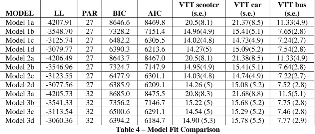
A comparison of the fit of the different models is provided in Table 4. This table reports, for each model, the number of parameters (PAR) and the final Log-Likelihood (LL), the Bayesian information criterion (BIC) (Schwarz, 1978) and the Akaike information criterion (AIC) (Akaike, 1974) measures to assess model fit.

MODEL LL PAR BIC AIC

VTT scooter (s.e.)

VTT car (s.e.)

VTT bus (s.e.)

Model 1a -4207.91 27 8646.6 8469.8 20.5(8.1) 21.37(8.5) 11.33(4.9)

Model 1b -3548.70 27 7328.2 7151.4 14.96(4.9) 15.41(5.1) 7.65(2.8)

Model 1c -3125.74 27 6482.2 6305.5 14.02(4.8) 14.73(4.9) 7.24(2.7)

Model 1d -3079.77 27 6390.3 6213.6 14.27(5) 15.09(5.2) 7.54(2.8)

Model 2a -4206.49 27 8643.7 8467.0 20.5(8.1) 21.38(8.5) 11.33(4.9)

Model 2b -3546.96 27 7324.7 7147.9 14.95(4.9) 15.41(5.1) 7.64(2.8)

Model 2c -3123.55 27 6477.9 6301.1 14.03(4.8) 14.74(4.9) 7.22(2.7)

Model 2d -3077.56 27 6385.9 6209.1 14.26 (5) 15.08 (5.2) 7.52 (2.8)

Model 3a -4205.73 32 8685.0 8475.5 20.8(8.3) 21.68(8.8) 11.5(5.1)

Model 3b -3541.33 32 7356.2 7146.7 15.22 (5) 15.68 (5.2) 7.75 (2.8) Model 3c -3113.54 32 6500.6 6291.1 14.54 (5) 15.29 (5.2) 7.46 (2.8) Model 3d -3060.36 32 6394.2 6184.7 14.90 (5.3) 15.78 (5.5) 7.77 (2.9)

Table 4 – Model Fit Comparison

The number of parameters in models 3a-3d is higher than in the other models due to the estimation of the parameters for the consideration probabilities. Both the Log-Likelihood and the AIC statistics suggest that model 3d fits the data best. The BIC penalises the additional parameters in the model more strongly and gives preference to model 2d, but this yields reduced insights into behaviour, and on balance, we therefore proceed with model 3d.

13

the mixing in Equation 4 then captures correlation across choices for the same person. In the treatment of availability, specification d always performs the best in each group, while, for consideration, we also as expected see that specification 3 always gives the better log-likelihood. Overall, any treatment of availability or consideration leads to improvements, but these differ across specifications.

The final three columns of Table 4 display value of travel time (VTT) measures obtained by computing the ratio between the mode-specific travel time coefficients and the cost coefficient. All the VTT measures are significantly different from zero and the standard errors are calculated using the delta method for this ratio. Within each model, the difference between car and scooter is not statistically significant (t-ratio of 1.14 in model 3d), while the difference with bus is (t-ratio of 5.45 for bus and scooter, and 5.70 for bus and car).

It is easy to notice how the models which do not include any availability nor consideration treatment (Models 1a, 2a and 3a) do not only provide a worse fit, but also excessively high VTT, while the other models provide more reasonable values, only slightly higher with respect to values computed in other studies with Italian data (Bickel et al., 2006) although comparison is difficult as a national value of travel time study has never been performed in Italy and therefore official data are unavailable.

As mentioned above, the 12 models described were estimated with the same utility specification, to control for the effect of the assumptions on availability and consideration. The final specification was obtained by starting off with a base model and systematically adding socio-demographic and trip-level variables to the utilities of the different choice alternatives on the basis of intuition and statistical significance. Due to space constraints, we cannot show the results of all the models (although these are available from the authors on request), so we only present the results for model 3d in Table 5. In order to correctly account for the panel nature of the data, robust t-ratios are reported alongside the estimates, where the log-likelihood entered the sandwich matrix calculations at the individual person level, i.e. grouping together choices and thus recognising the repeated choice nature of the data. Although the signs and magnitudes of the estimated parameters did not vary considerably across the different models, there are minor differences in the significance of the different coefficients, which results in some of them not being significant in the model presented.

Utility coefficients Mode Estimate Robust t-rat

Alternative-specific constants

Bicycle -1.931 -0.68

Scooter -4.930 -1.37

Car 1.244 0.43

Bus -2.552 -0.90

Distance Walk -3.453 -11.67

Bicycle -1.052 -4.40

Box-Cox parameters (Distance transformation)

Walk 0.198 0.94

Bicycle 0.695 4.60

Travel time

Scooter -0.263 -6.67

Car -0.278 -6.43

Bus -0.137 -5.30

Travel cost Scooter, car, bus -1.058 -3.41

Purpose = social Walk 0.707 2.40

14

Bicycle 1.126 2.91

Purpose=groceries Bicycle 1.076 2.37

Car 0.997 2.39

Weekday Car -0.585 -2.08

Rain Walk -0.357 -2.09

Bicycle -0.232 -1.14

Heavy rain Bus 0.698 1.71

Heat index Walk -0.044 -1.16

Scooter 0.059 1.74

Ascent ratio Bicycle -0.029 -0.95

Age 20-30 (base=older) Walk 0.997 1.66

Bicycle 1.301 2.43

Sex = male Scooter 0.445 1.38

Consideration probability coefficients

Distance Walk 5.874 3.08

Square of distance Walk -1.098 -3.18

Purpose=groceries Walk 5.064 1.35

Distance Bicycle -0.060 -0.32

Heat index Bicycle 0.027 2.09

Table 5 – Parameter estimates for model 3d

4.1 Utility Parameters

The first four coefficients in Table 5 are the alternative-specific constants for the modes, where walk is used a base. The travel time coefficients for motorised modes, as well as the cost coefficient, which enters the utility of motorised modes only, are negative and robustly significant. For walking and cycling, we work with distance rather than travel time, as time is a function of speed which is determined by physical ability and desire for exercise. We allow for non-linearity in the impact of distance on utility through a Box-Cox transform. The value of the Box-Cox parameters is below 1 for both modes, implying decreasing marginal sensitivity with increasing distance, where for walk, the value is not significantly different from 0, hence pointing towards a log shape. The distance coefficient for cycling is significantly different from 1 (robust t-ratio =-8.59), justifying the use of the transformation. With these values for the parameter and the Box-Cox parameter, the marginal disutility per kilometre is larger for walk than bicycle for the first 10 kilometres, while the marginal disutility caused by distance ‘crosses over’ (bicycle becoming more negative than walk) at a distance of about 44 kilometres, well outside the range where walking is likely to be considered in our model.

As mentioned in Section 2, participants annotated their trips with the purpose, which is found to have an impact on mode choice. We find that people are more likely to walk to social activities, which is not surprising, as the middle-sized city of Pisa and the small urban centres in its surrounding areas are easily walkable for most people. Probably for similar reasons, we find that walk and bicycle are more likely to be used for leisure activities, which include sports, going to the city centre, or visiting attractions. The utility of choosing car and bicycle, both modes that make it easy to transport goods, is higher for grocery shopping trips.

15

significant in this model. Heavy rain is associated with a preference for bus, a mode which provides shelter from the rain but also implies being able to avoid driving in difficult weather conditions. The area of analysis is characterised by mild winters and hot summers. High levels of the heat index discourage people from walking, as this is the slowest and most onerous mode in this context (although this coefficient is not significant in this model), but can make scooter very appealing, as this mode allows people to benefit from the wind without any physical effort. Although past literature has found evidence that weather conditions impact several aspects of travel behaviour, including mode choice (Cools & Creemers, 2013, Akar & Clifton 2009), we believe that these results are strongly related to the climate of the region, and should be interpreted using knowledge of the specific context. For example, Guo et al. (2007) find a strong weather effect in the case of Chicago, IL, but the ease of finding such an effect is also a factor of the variability in weather across days and seasons, which is much reduced in Pisa.

Another interesting coefficient, albeit not significant in the present model, is the fraction of the trip that implies going uphill. Prior studies showed how this variable negatively impacts the utility from non-motorised modes such as walking and cycling as this would increase the effort required (Rodrıguez & Joo, 2004, Cervero and Duncan, 2003). The reason for the lack of a stronger level of significance can be related to the fact that the city of Pisa and surrounding areas are rather flat, while of course an uphill outbound journey would imply a downhill return journey, cancelling the effect out and with a mode needing to be chosen for both.

Finally, we consider the effect of some socio-demographic characteristics. In line with expectations, younger people are found to be more likely to walk and cycle than older ones. In addition, a positive (although not strongly significant) correlation between being male and choosing scooter is found, in line with previous evidence from Italy (Bernetti et al., 2008).

4.2 Consideration Parameters

Models 3a-3d, differently from the preceding ones, imply the estimation of additional parameters due to the probabilistic approach to mode consideration discussed in the previous section. Table 5 displays the variables found to have an effect on the probability of consideration for model 3d. Trip distance was included in the expression of both modes. In the case of walk, we include both linear and squared distance. The signs and values of these coefficients imply that walk is considered with a probability of nearly 1 for short distances (cf. equation 7), but this decreases rapidly just below 5 kilometres, and the probability of considering walk goes to near 0 over 6 kilometres, a value that is close to the maximum distance where walk was chosen in the data. For grocery trips, this cut-off point is shifted slightly to the right, where this needs to be interpreted alongside the increases in utility for car and bicycle for grocery trips. For bicycle, the consideration model works less well, with only a small and statistically insignificant negative impact for distance, while consideration increases in warmer weather. As the data were collected starting in spring, this result could be interpreted by noting that, in a very flat context like Pisa, cycling might be a good option on warmer days.

5. Conclusions

16

The first research question that was proposed in the Introduction of this paper concerned the investigation of whether these passively collected data sources such as GPS can be used for travel behaviour modelling beyond route choice, in particular for mode choice modelling. We showed that this type of data, at least in our case, can indeed be used for this purpose, although special care needs to be taken in understanding, cleaning, enriching and handling the data.

Our second question revolved around finding ways to deal with the issue of mode availability and consideration. In our case, as in many similar datasets, the lack of information about person-level mode availability requires them to be inferred, which can be done by using other socio-demographic information if available. This method proved not only effective, but superior to the use of stated availabilities, suggesting that inferred information can be more reliable than what is stated by respondents, as it allows for some uncertainty compared to simple 0/1 availability. In addition, the inclusion of a consideration set seems to provide an improvement in model fit, showing that real-life behaviour is better represented if this additional layer is added to the choice set formation process. Our findings thus suggest that a better understanding of modes choices can be obtained by looking jointly at availability, consideration and choice.

Despite the challenges faced when trying to model this type of data, the gains in terms of understanding of behaviour can be considerable. Not only can capturing the complexity of real-world behaviour provide better measures of sensitivities to different influencing factors, but it also allows us to address the biases of SP data by comparing the outcomes of models estimated with different data sources. Notwithstanding the challenges discussed, the present paper serves as a proof of concept that the use of data collected by passive data sources for various purposes could be a valuable resource for travel behaviour modelling. This is confirmed by reasonable model results, including a realistic estimate of the monetary value of travel time. The current research needs to be followed by confirmatory analyses with different datasets, including comparison with SP data (which has its own limitations) for value of time research.

Acknowledgments

The Leeds authors acknowledge the financial support by the European Research Council through the consolidator grant 615596-DECISIONS. The last author acknowledges the partial support by the European Community’s H2020 Program under the scheme ‘INFRAIA -1-2014-2015: Research Infrastructures’, grant agreement 654024 ‘SoBigData: Social Mining & Big Data Ecosystem’.

References

ACI (Automobile Club d'Italia), 2014. Costi Chilometrici. Url: http://www.aci.it

Akaike, H. (1974), A new look at the statistical model identification, IEEE Transactions on Automatic Control, 19 (6): 716–723

Akar, G., & Clifton, K. (2009). Influence of individual perceptions and bicycle infrastructure on decision to bike. Transportation Research Record: Journal of the Transportation Research Board, (2140), 165-172.

Archivio Meteo Pisa. Url: www.ilmeteo.it

17

Bickel, P., Friedrich, R., Burgess, A., Fagiani, P., Hunt, A., Jong, G., Laird, J., Lieb, C., Lindberg, G., Mackie, P., et al. (2006). Heatco–developing harmonised european approaches for transport costing and project assessment. IER University Stuttgart Bierlaire, M., & Frejinger, E. (2008). Route choice modeling with network-free data.

Transportation Research Part C: Emerging Technologies, 16(2), 187-198.

Bierlaire, M., Chen, J., & Newman, J. (2010). Modeling route choice behavior from smartphone GPS data. Report TRANSP-OR, 101016, 2010.

Bohte, W., & Maat, K. (2009). Deriving and validating trip purposes and travel modes for multi-day GPS-based travel surveys: A large-scale application in the Netherlands. Transportation Research Part C: Emerging Technologies, 17, 285-297.

Broach, J., Dill, J., & Gliebe, J. (2012). Where do cyclists ride? A route choice model developed with revealed preference GPS data. Transportation Research Part A: Policy and Practice, 46(10), 1730-1740.

Cantillo, V., & Ortúzar, J. de D. (2005). A semi-compensatory discrete choice model with explicit attribute thresholds of perception. Transportation Research Part B: Methodological, 39(7), 641-657.

Casas, J. and Arce, C. (1999). Trip reporting in household travel diaries: A comparison to gps-collected data. In 78th annual meeting of the Transportation Research Board, Washington, DC, volume 428.

Cascetta, E., & Papola, A. (2001). Random utility models with implicit availability/perception of choice alternatives for the simulation of travel demand. Transportation Research Part C: Emerging Technologies, 9(4), 249-263.

Cervero, R. and Duncan, M. (2003). Walking, bicycling, and urban landscapes: evidence from the San Francisco Bay Area. American journal of public health 93.9: 1478-1483. Chen, C., Gong, H., Lawson, C., & Bialostozky, E. (2010). Evaluating the feasibility of a

passive travel survey collection in a complex urban environment: Lessons learned from the New York City case study. Transportation Research Part A: Policy and Practice, 44(10), 830-840.

Computer programme to calculate emissions from road transport, Copert 4 version 8.0; 2010. <http://www.emisia.com/copert/>.

Cools, M. and Creemers, L. (2013). The dual role of weather forecasts on changes in activity-travel behavior, Journal of Transport Geography, 28:167-175

Cottrill, C., Pereira, F., Zhao, F., Dias, I., Lim, H., Ben-Akiva, M., & Zegras, P. (2013). Future mobility survey: Experience in developing a smartphone-based travel survey in singapore. Transportation Research Record: Journal of the Transportation Research Board, (2354), 59-67.

Dhakar, N. and Srinivasan, S. (2014). Route choice modeling using gps-based travel surveys. Transportation Research Record: Journal of the Transportation Research Board, 2413:65–73.

Feng, T. & Timmermans, H.J.P. (2015). Enhanced imputation of GPS traces forcing full or partial consistency in activity-travel sequences: comparison of algorithms. Transportation Research Record, 2430, 20-27.

18

GPS.gov (2016). Official U.S. Government information about the Global Positioning System (GPS) and related topics. Url: http://www.gps.gov/. Maintained by the National Coordination Office for Space-Based Positioning, Navigation and Timing.

Greaves, S. P., Ellison, A. B., Ellison, R. B., Rance, D., Standen, C., Rissel, C., and Crane, M. (2014). A web-based diary and companion smartphone app for travel/activity surveys. In International Conference on Transport Survey Methods.

Hess, S., Quddus, M., Rieser-Schüssler, N., and Daly, A. (2015). Developing advanced route choice models for heavy goods vehicles using gps data. Transportation Research Part E: Logistics and Transportation Review, 77:29–44.

Hess, S. "Latent class structures: taste heterogeneity and beyond." Handbook of Choice Modelling (2014): 311.

Hotho, A., Pedersen, R. U., & Wurst, M. (2010). Ubiquitous data. In Ubiquitous knowledge discovery (pp. 61-74). Springer Berlin Heidelberg.

Huang, A., & Levinson, D. (2015). Axis of travel: Modeling non-work destination choice with GPS data. Transportation Research Part C: Emerging Technologies.

Iqbal M. S., Siddique M. A., Islam M., Choudhury C. (2013), Predicting Tour Patterns Derived from Ubiquitous Data Sources, Transportation Research Board Annual Meeting, January 2013.

Jariyasunant, J., Carrel, A., Ekambaram, V., Gaker, D. J., Kote, T., Sengupta, R., & Walker, J. L. (2011). The Quantified Traveler: Using personal travel data to promote sustainable transport behavior. University of California Transportation Center.

Kamakura, W. A., Russell, G., 1989. A probabilistic choice model for market segmentation and elasticity structure. Journal of Marketing Research 26, 379-390.

Kelly, P., Krenn, P., Titze, S., Stopher, P., & Foster, C. (2013). Quantifying the difference between self-reported and global positioning systems-measured journey durations: a systematic review. Transport Reviews, 33(4), 443-459.

Manski, C. F. (1977). The structure of random utility models. Theory and decision, 8(3), 229-254.

Map Data © 2016 Google

McFadden, D., 1974. Conditional logit analysis of qualitative choice behaviour. In: Zarembka, P. (Ed.), Frontiers in Econometrics. Academic Press, New York, pp. 105-142.

Miyashita, K., Terada, T., & Nishio, S. (2008). A map matching algorithm for car navigation systems that predict user destination. In Advanced Information Networking and Applications-Workshops, 2008. AINAW 2008. 22nd International Conference on (pp. 1551-1556). IEEE.

Prato, C. G. (2009). Route choice modeling: past, present and future research directions. Journal of Choice Modelling, 2(1), 65-100.

Quddus, M. A., Ochieng, W. Y., & Noland, R. B. (2007). Current map-matching algorithms for transport applications: State-of-the art and future research directions. Transportation Research Part C: Emerging Technologies, 15(5), 312-328.

Quiroga, C., Perez, M., and Venglar, S. (2002). Tool for Measuring Travel Time and Delay on Arterial Corridors, chapter 75, pages 600–607.

19

R Core Team (2016). R: A Language and Environment for Statistical Computing, for R Foundation for Statistical Computing, Vienna, Austria. URL: https://www.R-project.org.

Safi, H., Assemi, B., Mesbah, M., Ferreira, L., & Hickman, M. (2015). Design and implementation of a smartphone-based travel survey. Transportation Research Record: Journal of the Transportation Research Board, (2526), 99-107.

Schuessler, N., & Axhausen, K. (2009). Processing raw data from global positioning systems without additional information. Transportation Research Record: Journal of the Transportation Research Board, 2105, 28-36.

Schwarz, Gideon E. (1978), "Estimating the dimension of a model", Annals of Statistics, 6 (2): 461–464

Shen, L., & Stopher, P. R. (2013). A process for trip purpose imputation from Global Positioning System data. Transportation Research Part C: Emerging Technologies, 36, 261-267.

Statistiche dell'Energia, Ministero dello sviluppo economico. Url: http://dgsaie.mise.gov.it/dgerm/prezzimedi.asp?prodcod=1&anno=2014

Stopher PR, Zhang J, Zhang Y and Halling B 2009 'Results of an Evaluation of TravelSmart in South Australia', 32nd Australasian Transport Research Forum ATRF 2009, Auckland, New Zealand, 1st October 2009

Stopher, P., Clifford, E., Zhang, J., and FitzGerald, C. (2008). Deducing mode and purpose from GPS data. Institute of Transport and Logistics Studies.

Stopher, P. (2012). Collecting, managing, and assessing data using sample surveys. Cambridge University Press.

Stopher, P., & Wargelin, L. (2010). Conducting a household travel survey with GPS: reports on a pilot study. In 12th World Conference on Transport Research (pp. 11-15).

Swait, J. (2001) Choice set generation within the generalized extreme value family of discrete choice models. Transportation Research Part B: Methodological, 35(7), 643-666. Swait, J., & Ben-Akiva, M. (1987). Incorporating random constraints in discrete models of

choice set generation. Transportation Research Part B: Methodological, 21(2), 91-102. Tsui, S. Y. A, Shalaby, A. S. (2006). An Enhanced System for Link and Mode Identification

for GPS-based Personal Travel Surveys. Proceedings of the 85th Annual Meeting of the Transportation Research Board, January 2006, Washington D.C.