1
Interaction of Vortex Shedding Processes on Flow over a
1Deep-Draft Semi-Submersible
2Yibo Liang, Longbin Tao* 3
School of Marine Science and Technology, Newcastle University, Newcastle upon Tyne, NE1 7RU, 4
UK 5
Abstract
6
A numerical study on the flow over a Deep-Draft Semi-Submersible (DDS) for both stationary and 7
Vortex-Induced Motions (VIM) was carried out using the Computational Fluid Dynamics (CFD), with 8
the aim to investigate the overall hydrodynamics of the structure. In order to study the fluid physics 9
associated with VIM, a comprehensive numerical simulation was conducted to examine the 10
characteristics of vortex formations, shedding processes and especially their interactions due to the 11
multiple cylindrical columns. In addition to the vortex shedding characteristics, the drag and lift 12
forces on each member of the overall structure were calculated. It is revealed that under 45° 13
incidence, the transverse forces induced by the portside and starboard side columns are the dominant 14
excitation forces responsible to VIM while the horizontal member - pontoons restraining VIM. In 15
addition, the hysteresis phenomenon observed between the force and motion domains - the peak lift 16
force occurs slightly earlier than the peak transverse motion is mainly due to the vortices shed from 17
the upstream column move back to impinge on one of the side columns after impinging on the other 18
side column and the symmetrical strong vortices which shed from the side columns. 19
Keywords
20
*Corresponding author. Tel.: +44 (0) 191 208 6670; Fax: +44 (0) 191 208 5491; E-mail address:
2 Vortex-Induced Motions (VIM); Deep-Draft Semi-Submersible (DDS); Computational Fluid
21
Dynamics (CFD) 22
Nomenclature
23
Ax/L Non-dimensional characteristics amplitude of in-line motion 24
Ay/L Non-dimensional characteristics amplitude of transverse motion
25
BL Platform width 26
BT Platform draft
27
Ca Added mass coefficient 28
CD Drag force coefficient 29
CL Lift force coefficient
30
D Column projected length 31
f Vortex shedding frequency 32
f0 Natural frequency in still water 33
Fr Froude number 34
FD Hydrodynamic drag force acting on the structure 35
FL,Fy Hydrodynamic lift force acting on the structure
36
GCI Grid convergence index 37
H Immersed column height above the pontoon 38
L Column width 39
m Platform mass 40
ma Added mass
41
P Pontoon height 42
Re Reynolds number 43
rms Root mean square 44
S Distance between centre columns 45
St Strouhal number 46
T0 Natural periods in still water 47
∆t Numerical simulation time step 48
U,Uc Current speed
49
Ur Reduced velocity 50
3 ∆ Displacement
52
λ Scale ratio 53
ω
⃑⃑ x Streamwise vorticity
54 ω
⃑⃑ y Transverse vorticity
55 ω
⃑⃑ z Spanwise vorticity
56
X In-line motion 57
Y Transverse motion 58
y+ Y plus value
59
1.
Introduction
60
Vortex-Induced Motions (VIM) have been receiving continuous attention in the field of offshore 61
exploration and exploitation as an increasing number of deep-draft floating structures have been 62
operating in different regions around world. Deep-draft floating structures are well known for their 63
favourable vertical motions behaviour compared with other types of floating offshore structures. 64
However, the increases in the structure’s draft can also lead to more severe VIM, which may lead to 65
potential damage particularly causing fatigue to the mooring and riser systems. 66
VIM have often been observed since the Genesis Spar platform was commissioned in 1997 (Fujarra et 67
al., 2012; Kokkinis et al., 2004). Rijken and Leverette (2009) reported VIM phenomenon on a semi-68
submersible in field measurements. Ma et al. (2013) also observed the presence of VIM from recent 69
field measurements. In this aspect, a number of studies on the VIM behaviours have been carried out, 70
including both experimental and numerical studies. On the experimental investigation side, as pointed 71
out by Fujarra et al. (2012) in their comprehensive review, VIM are now much better understood. 72
However, it is still lack of understanding about the VIM mechanism on multiple cylindrical structures 73
such as the semi-submersible and the Tension-Leg Platform (TLP). The vortex shedding processes 74
and subsequent VIM are much more complex than those of single cylindrical structures due to the 75
multi-columns, pontoons and their interactions with the vortex shedding processes. 76
Waals et al. (2007) conducted several VIM tests on both DDS and TLP to examine the influences of 77
4 and the results showed that under a strong current, the DDS will have more significant VIM responses 79
compared with the wave-current coupling condition. Rijken and Leverette (2008) experimentally 80
studied the VIM responses of a DDS, and observed that wave and external damping can affect the 81
VIM responses. Through their tests, it was noted that the relatively low sea states do not particularly 82
influence the VIM responses under the so-called “lock-in” region. Moreover, the additional damping 83
delayed the onset of VIM to a higher reduced velocity. Rijken et al. (2011) analysed the influences of 84
SCR systems and appurtenances on VIM for a DDS. Their work showed that the appurtenances on the 85
vertical faces of the columns and above the pontoon can alter the VIM responses. Gonçalves et al. 86
(2012) subsequently investigated the effects of the current angle and appendages on a conventional 87
semi-submersible. The presence of VIM on a conventional semi-submersible has been confirmed in 88
their works. Following on from their initial outcomes, Gonçalves et al. (2013) further studied other 89
relevant factors such as the draft conditions, the external damping and wave effects on VIM 90
developing by performing a series of towing tank tests. Additionally, Gonçalves et al. (2015) 91
performed experimental tests focusing on the effects of different column designs on the VIM 92
responses. The results showed that the circle section shaped column design has the most severe 93
transverse motions at 0 degree flow incidence and that the square section shaped column design has 94
the most significant transverse motion at 45 degree flow incidence. Recently, Antony et al. (2016) 95
studied the effects of damping on VIM and investigated the force distribution on each member of the 96
structure in detail by an experimental routine. The work done by each member was presented in their 97
investigations. The investigations showed that for 45 degree flow incidence, when the maximum 98
transverse VIM response occurs, three upstream columns excited VIM. The horizontal member - 99
pontoons, however, were noted to limit the VIM responses. 100
In the last decade, the continued technological advances offer ever-increasing computational power, 101
in which CFD methods are rapidly gaining popularity for VIM predictions. Lefevre et al. (2013) 102
proposed the guidelines for undertaking the Spar VIM simulations. Tan et al. (2013) performed a 103
series of CFD simulations for VIM on a multi-column floater. Lee et al. (2014) studied the differences 104
5 numerically and experimentally investigated the VIM responses of a deep-draft column stabilized 106
floater. Their work shows that the damping effects of the riser and mooring systems are very 107
important in CFD simulations. Vinayan et al. (2015) increased the confidence for CFD simulations on 108
the VIM predictions of a deep-draft column stabilized floater through a series of numerical 109
simulations on a PC-semi with different drafts and arrangements. Liu et al. (2015) numerically 110
investigated the effects of pontoon on hydrodynamic forces for a stationary DDS model and revealed 111
that the DDS with the different numbers of pontoons affects both drag and lift forces on the stationary 112
structures. Koop et al. (2016) carried out a series of CFD studies to illustrate the results of the scale 113
and damping effects for VIM on a semi-submersible. Their work showed that the scale effects at 45 114
degree incidence are less than that at 0 degree incidence. Under 45 degree incidence, the VIM 115
response at prototype Reynolds number is found to be similar compared with that at model scale 116
Reynolds number. Similar observation was also reported by Lee et al. (2014). 117
2.
Numerical simulation
118
2.1. Computational overview 119
A comprehensive numerical study was conducted in this section, with the aim to examine the vortex 120
shedding characteristics and the associated fluid dynamics. The numerical schemes are introduced and 121
followed by a sensitivity assessment in order to perform a computationally efficient numerical 122
analysis. 123
The Detached Eddy Simulation (DES) method was used in this study. For the DES model, the 124
Improved Delayed Detached Eddy Simulation (IDDES) model (Shur et al., 2008) with the Spalart-125
Almaras (SA) (Spalart et al., 1997) was used. All the simulations were carried out by using a Star-126
CCM+ 9 package. 127
The principle dimensions of the deep-draft semi-submersible analysed in this section are given in 128
6 conditions ranging from Reynolds number 3×10⁵ to 1.1×10⁶. Model I is used for the stationary 130
structure simulations where the model scale ratio is 1:128. Model II is for the VIM simulations where 131
the model scale ratio is 1:64. For all simulations, the computational domain 9BL×6BL×3BT is used
132
(where BL is the overall hull width of the semi-submersible and BT is the draft of the semi-133
submersible) based on the convergence study. The computational domain were 6BL×4.5BL×2.8BT
134
and 5BL×4BL×2.2BT in the studies by Lee et al. (2014). Tan et al. (2013) performed their analysis
135
using a 27BL×18BL×6.5BT domain and Liu et al. (2015) used a 11BL×6BL×3BT domain. Koop et 136
al. (2016) chose a 10BL ×6BT cylindrical domain. Compared with aforementioned computational 137
domain sizes, a 9BL×6BL×3BT domain (see Fig. 2) was considered to be large enough to eliminate
138
the far field effects from the boundaries and the three-dimensional effects from a spanwise cross flow 139
direction. 140
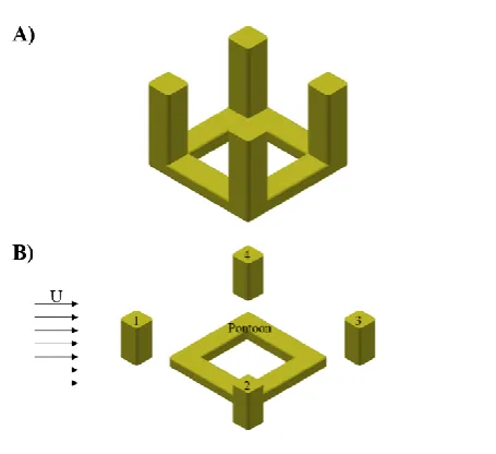
[image:6.595.185.413.368.576.2]141
Fig. 1. The DDS model (A is the entire model and B is the decomposed model which show the 142
definition of the individual members). 143
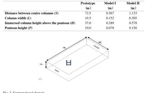
Table 1. Main characteristics of the DDS unit (The model I is the stationary model which presents 144
7
Prototype
(m)
Model I
(m)
Model II
(m)
Distance between centre columns (S) 72.5 0.567 1.133
Column width (L) 19.5 0.152 0.305
Immersed column height above the pontoon (H) 37.0 0.289 0.578
Pontoon height (P) 10.0 0.078 0.156
[image:7.595.62.526.69.368.2]146
Fig. 2. Computational domain. 147
The polyhedral mesh (CD-adapco, 2014) was used in the present study. The overall elements mesh is 148
shown at a middle-depth horizontal layer in Fig. 3. In the present study, a near wall refinement 149
method named “Prism Layer Mesher” is adopted. The y+ values are smaller than 1 in all simulations,
150
wherey+=u*∆y1/ν (u* denotes the friction velocity at the nearest wall, ∆y1 is the first layer thickness
151
and ν is the kinematic viscosity). Other five regional refinements are carried out in the domain to 152
refine both the near wake and the far wake region (see Fig. 4). 153
The boundary conditions are kept all the same in the present study. At the inlet, a uniform and 154
constant velocity is specified directly for all sensitivity studies. The pressure at boundary was 155
extrapolated from the adjacent cell using reconstruction gradients (CD-adapco, 2014). Along the 156
outlet boundary, the pressure is prescribed to be equal to zero. The velocity at the boundary was 157
extrapolated from the interior using reconstruction gradients (CD-adapco, 2014). For the body surface 158
of the deep-draft semi-submersible, a no-slip boundary condition was specified in terms of the 159
tangential velocity which is explicitly set to be zero and the pressure at the boundary was extrapolated 160
8 quite small (Fr < 0.2) in all simulations, the free surface effects can be ignored and the free surface 162
boundary condition is prescribed as being a symmetry boundary. 163
164
Fig. 3. Visualisation of the mesh at the middle draft level of the DDS (XY plane at the middle draft of 165
the DDS). 166
2.2. Sensitivity studies 167
In order to investigate the numerical mesh sensitivity of the calculated results, a mesh sensitivity 168
study had been carried out with different levels of refinement grids resolution following the guideline 169
proposed by Celik et al. (2008). The Reynolds number set for the mesh sensitivity study is 1.1×10⁶, 170
which is the highest Reynolds number in all the undertaken simulations. The details of the mesh 171
sensitivity studies are shown in Table 2. Results for all cases are obtained by averaging after more 172
than fifteen vortex shedding cycles. 173
Table 2. Calculations of discretization error (Celik et al., 2008); GCI index represents the numerical 174
uncertainty. 175
C
̅D CLrms St
N1, N2, N3
(thousand)
6860, 3430, 937 6860, 3430, 937 6860, 3430, 937
r21 1.333 1.333 1.333
r32 1.6 1.6 1.6
∅1 1.066 0.093 0.131
∅2 1.068 0.101 0.131
∅3 1.053 0.139 0.134
9 GCInormal32 0.23% 18.31% NaN
GCIfine21 0.09% 9.13% NaN
Following the guideline proposed by Celik et al. (2008), N3, N2, N1 represent the total number of grids
176
from a course grid refinement level to a relatively fine grid refinement; r is the grid refinement factor, 177
where r= hcoarse⁄hfine and h is the grid size; Ø is the calculation results for different grid refinements;
178
p is the apparent order; GCI is the grid convergence index which shows the level of numerical 179
uncertainty. The resulting force coefficients (CD, CL) and the Strouhal number (St) which are
180
compared in the sensitivity studies are defined as: 181
CD= 1FD 2ρUC
2A, (1)
182
CL= 1FL 2ρUC2A
, (2) 183
St= UfL
c, (3)
184
where, FD is the drag force on the structure, FL is the lift force on the structure, ρ is the fresh water
185
density, UC is the free stream velocity, A is the projected area of the immersed structure, f is the 186
vortex shedding frequency obtained from the power spectra of lift force coefficient fluctuations as 187
followed by Schewe (1983) and L is the width of the DDS column. 188
As shown in Table 2, there is a reduction in the GCI index for the successive finer grid refinements, 189
where GCIfine21 is less than GCInormal32 . The GCI index for the fine grid refinement (GCIfine21 ) is relatively 190
low compared to the coarse level of grid refinement (GCInormal32 ), indicating that the dependence of the 191
numerical simulation on the mesh has been reduced. As the GCI index reduction from the coarse grid 192
refinement to the fine grid refinement is relatively high, then the mesh convergence (grid 193
independent) can be said to have been nearly achieved. Additionally, as the St may indicate that the 194
10 performed in Fig. 4. It shows that the St is converged around the value of 0.131. Therefore, the
196
numerical uncertainty for the Strouhal number is shown as “NaN” in Table 2. These mesh sensitivity 197
studies show that the N2 numerical mesh setting is fine enough to obtain reliable results with an 198
acceptable computation time and they are used in further numerical studies. 199
200
Fig. 4. Calculations with additional grid refinements for the Strouhal number (St). 201
The non-dimensional time step is chosen as 0.008 (non-dimensional time step = ∆tU/L, where ∆t is 202
the time step, U is the inlet velocity and L is the width of the DDS column) for all cases based on 203
sensitivity test. The constant non-dimensional time step size will result in varying courant (CFL) 204
numbers as the grid is refined. A major benefit of employing the IDDES approach is that a large 205
portion of the flow should be resolved with the Large Eddy Simulation (LES), but this requires rather 206
strict CFL number limits. In the present study, the CFL numbers for the majority of the overall flow 207
region are less than 1. Only in some tiny flow areas, the CFL numbers are found to be between 1 to 2. 208
Therefore, the time step is considered to be fine enough for the current simulations’ requirement 209
(Liang et al., 2016). 210
2.3. Reduced velocity 211
When discussing VIM, the so-called reduced velocity (Ur) is usually used as the reference value. The 212
11 Ur= UT0
D , (4)
214
where U is the current speed, T0 is the natural period of the motions in calm water and D is the 215
projected length of the column. 216
3.
Results and discussion
217
Two different conditions (stationary and VIM) of a typical deep-draft semi-submersible under 45 218
degree flow incidence were investigated using the present numerical model and their results are 219
further compared with the experimental data from model tests conducted in a circulating water 220
channel and a towing tank respectively. 221
The results from both previous works and present outcomes are summarised in Table 3. As confirmed 222
in both field measurements and model tests (Gonçalves et al., 2012; Koop et al., 2016; Lee et al., 223
2014; Ma et al., 2013; Magee et al., 2011; Rijken and Leverette, 2008; Waals et al., 2007), for square 224
section shaped multi-columns structures, the most severe transverse motion occurred at 45 degree 225
incidence. As Koop et al. (2016) noted, the scale effects of a DDS in a 45 degree flow are less than 226
that in a 0 degree flow. This indicates that the Reynolds number does not have a large effect on the 227
model predictions at 45 degree incidence. Aiming to investigate the VIM of a DDS at a realistic field 228
condition with the real engineering applications, the flow over a stationary structure and a VIM model 229
of a DDS at 45 degree incidence have been numerically investigated after a rigorous validation 230
against the experimental data. The hydrodynamic loads on different members of the structure, such as 231
four columns and pontoons, are compared in order to quantify the determining factors which induced 232
VIM excitation. Moreover, the flow patterns are further examined to reveal the insights of the vortex 233
dynamics associated with VIM. 234
Table 3. Summary of the various studies on VIM of the multiple square section shaped columns 235
12
λ H/L Ur max Ay/L at 0° max Ay/L at 45°
Waals et al. (2007) 1:70 1.75 4.0~40.0 -- 0.320
Rijken and Leverette (2008) 1:50 2.18 1.0~15.0 0.151 0.468
Magee et al. (2011) 1:70 1.50 4.0~13.0 0.269 0.319
Gonçalves et al. (2012) 1:100 1.14 2.5~20.0 0.268 0.382
Ma et al. (2013) 1:1 -- 3.2~13.7 0.163 0.218
Lee et al. (2014) 1:67 1.78 4.0~20.0 -- 0.393
Lee et al. (2014) 1:1 1.78 4.0~20.0 -- 0.344
Koop et al. (2016) 1:54 -- 3.0~10.0 -- 0.470
Present work 1:64 1.90 3.4~14.1 0.279 0.742
237
3.1. “lock-in” phenomenon 238
The “lock-in” phenomenon is defined as being the synchronized oscillation region that is experienced 239
as VIM develops. When flow over a bluff body, vortices are generated on the downstream area of the 240
structure which are detached periodically and alternately from each opposite sides of the structure. 241
The structure affected by the vortex shedding may thus begin oscillating either side to side or in a fore 242
and aft manner. If the vortex shedding frequency closes to the natural frequency of the structure, the 243
motion can be amplified. This amplification phenomenon is named as the “lock-in”. The “lock-in” 244
always happened at reduced velocity around seven (See Fig. 5). It can be clearly seen in Fig. 5 that the 245
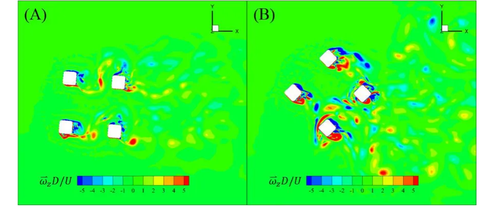
structure experiences the largest transverse motions at 45 degree incidence. Fig. 6 shows the spanwise 246
vorticity contour (ω⃑⃑ zD/U) when the “lock-in” generated. Under 45 degree incidence, the
non-247
dimensional spanwise vorticity is stronger than that under 0 degree incidence. In the present 248
investigation, the hydrodynamic loads on the structures and the vortex shedding interactions under 45 249
13 251
Fig. 5. Non-dimensional transverse characteristic amplitudes (Ay⁄L) obtained from the present towing
252
tank test. 253
254
Fig. 6. Non-dimensional spanwise vorticity (ω⃑⃑ zD/U) contours around the DDS at middle draft
255
showing the flow fields when “lock-in” has occurred (A: Ur = 6.4, 0 degree incidence. B: Ur = 6.6, 45 256
degree incidence). 257
3.2. Stationary model results and observations 258
In this section, a numerical study of the flow over a stationary deep-draft semi-submersible model 259
14 overall hydrodynamics. Results for all cases were obtained by averaging after more than fifteen vortex 261
shedding cycles. These numerical predictions are subsequently validated by the force measurements 262
from the corresponding experimental measurements which have been undertaken in a circulating 263
water channel. The characteristics of vortex shedding processes and their interactions due to the 264
multiple cylindrical column arrangement are examined in detail. 265
3.2.1. Overall drag and lift forces on the DDS 266
The overall fluid drag and lift forces are presented as the non-dimensional force coefficients CD and
267
CL. Details of the numerical results are given in Table 4. 268
Table 4. The resulting force coefficient values C̅D, CLrms and St for the flow over a stationary DDS. 269
Re
C
̅
D CLrms St3.7
×
10
4 1.068 0.070 0.1404.3
×
10
4 1.046 0.069 0.1385.2
×
10
4 1.044 0.066 0.1436.0
×
10
4 1.053 0.080 0.142These numerical results are validated by the force measurements obtained from the corresponding 270
experimental data. The experiments were conducted in a circulating water channel. The circulating 271
water channel is vertically oriented with an 8.0m length, 3.0m width and 1.6m depth measuring 272
section. The range of the flow velocity is 0.1 ~ 3m/s, and the minimum fluctuations of the current 273
velocity speed is 0.01m/s. The total fluid forces on the model I was measured by a three-component 274
force transducer. 275
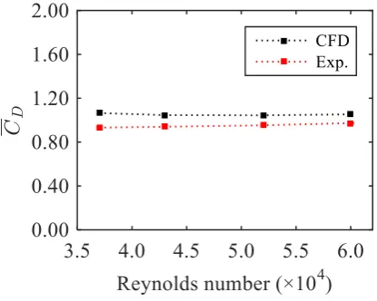
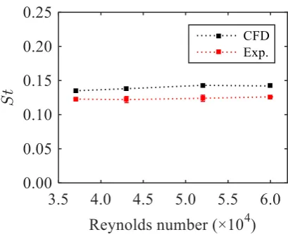
Comparisons between the results from the numerical simulations and the experimental measurements 276
are shown in Fig. 7, Fig. 8 and Fig. 9. The numerical predictions for the mean drag coefficient (C̅D), 277
the root mean square lift force coefficient (CLrms) and the Strouhal number (St) all show good 278
agreements when compared with the experimental data. The drag and lift force coefficients on the 279
15 Strouhal number (St) is around 0.14 which is similar to the results from the CFD study carried out by 281
Lee et al. (2014). 282
283
Fig. 7. Mean drag coefficient (C̅D) from the numerical and experimental results for the stationary 284
model. 285
[image:15.595.184.392.148.314.2]286
Fig. 8. Root mean square lift coefficient (CLrms) from the numerical and experimental results for the
287
16 289
Fig. 9. Strouhal number (St) from the numerical and experimental results for the stationary model. 290
3.2.2. Drag and lift forces on each member of the DDS 291
In order to improve the understanding of interactions between vortex shedding processes due to each 292
structure member of the DDS, the drag and lift force coefficients on each member of the DDS are 293
calculated and presented in Fig. 10, Fig. 11 and Fig. 12. The mean drag coefficients on each member 294
remain stable within the current Reynolds number range similar to the trend of the overall mean drag 295
coefficients on the DDS as discussed in the above section. Respectively, the upstream column 296
(Column 1) experiences a larger mean drag coefficient (C̅D) than the downstream one (Column 3). 297
The portside and starboard side columns (Column 2 and 4) are symmetrically expose to the flow and 298
experience a slightly larger mean drag coefficient (C̅D) than the upstream column, and the pontoon 299
shows the same trend as the side columns do. It is noted that the downstream column and the two side 300
columns are subjected to higher fluctuating lift force coefficient than the upstream one with the 301
downstream column experiencing the largest fluctuating lift force coefficient among all parts of the 302
DDS. The root mean square lift force coefficients on the two side columns are slightly less than that 303
on the downstream one, but still much larger than that on the upstream column. These results show 304
the influence of unsteady vortices and their interactions on the structure members in the downstream. 305
17 307
Fig. 10. Mean drag coefficients (C̅D) on each member of the stationary DDS. 308
[image:17.595.183.412.572.732.2]309
Fig. 11. Root mean square lift coefficients (CLrms) on each member of the stationary DDS.
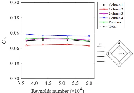
310
18 Fig. 12. Mean lift coefficient (C̅L) on each member of the stationary DDS.
312
3.2.3. Flow patterns and the lift force time history 313
With the aim to reveal the force dynamic behaviours on the structure, the time histories of the lift 314
force coefficients corresponding with the flow patterns at Re=4.3×10⁴ are presented in Fig. 13, Fig. 315
14 and Fig. 15. 316
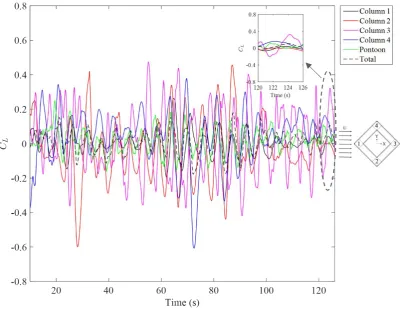
[image:18.595.93.496.275.596.2]317
Fig. 13. Lift force coefficient time history on different members of the DDS at Re=4.3×10⁴, 318
including locally zoomed in the last 6s. 319
As can be seen in Fig. 13, the time history of the lift force coefficient on column 3 shows a hysteresis 320
phenomenon which indicates the lift force oscillating period on column 3 always delayed compared 321
19 corresponded to the bottom values of other structure members, and vice versa. From the pressure 323
contours (Fig. 14), it can be clearly observed that there is a relatively stationary high pressure zone in 324
front of column 1, 2 and 4. However, the high pressure zone in front of the downstream column 3 325
keeps changing along with the vortex shedding processes. The fluctuations of the pressure in front of 326
column are primarily induced by the impingement of the upstream generated vortices, and these 327
fluctuations of the pressures cause the downstream column 3 to have higher CLrms and lower C̅D
328
values compared with other three upstream columns. On the other hand, the pressure fluctuations in 329
front of column 3 are mainly resulted in the interaction between the vortices shed from the upstream 330
[image:19.595.72.528.365.776.2]column 1 and the shear layers separated from the downstream column 3, which can be clearly seen in 331
Fig. 15. Similar observations were also noted by Ljungkrona et al. (1991), Chen and Chiou (1997) and 332
Liu and Chen (2002). 333
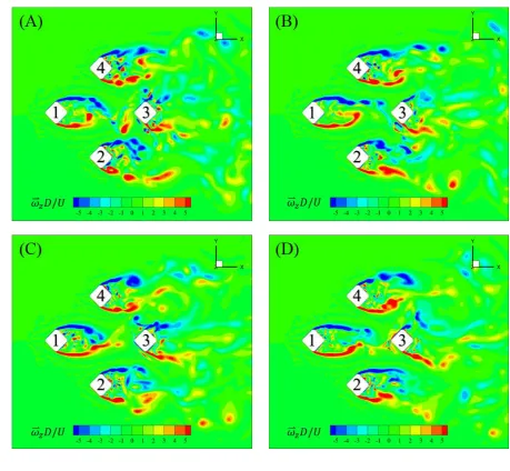
20 Fig. 14. A time series of the pressure distribution around the DDS at middle draft showing the
335
instantaneous flow fields around the DDS at Re=4.3×10⁴ corresponding to the lift force coefficient 336
time history (A: 120.6s; B: 122.4s; C: 124.2s; D: 126.0s). 337
[image:20.595.63.523.165.589.2]338
Fig. 15. A time series of non-dimensional spanwise vorticity (ω⃑⃑ zD/U) contours around the DDS at the
339
middle draft level showing the instantaneous flow fields around the DDS at Re=4.3×10⁴ 340
corresponding to the lift force coefficient time history (A: 120.6s; B: 122.4s; C: 124.2s; D: 126.0s). 341
Fig. 15 also shows that the vortex shedding patterns due to each column are very different. It is seen 342
that very slim vortices are shed from the corners of column 1. However, the vortices shed from the 343
21 even shorter vortices shed from the corners of downstream column 3 are clearly visible. Moreover, 345
column 2 and column 4 shed the large vortices symmetrically, where column 2 shed the vortices on its 346
portside corner and the column 4 shed on its starboard side corner. This symmetrical vortex shedding 347
pattern contributes to the symmetrical values of C̅L for column 2 and column 4 as shown in Fig. 12. 348
3.3. VIM model results and observations 349
After studying the vortex shedding interactions with the columns for the flow over a stationary 350
structure, a VIM investigation was carried out, in order to reveal the cause of VIM by comparing the 351
forces distributions and the flow patterns differences between the flow over the motion-coupled 352
structure cases with the stationary structure cases. 353
In this section, the numerical simulations of the flow over a three degree of freedom deep-draft semi-354
submersible model with different Reynolds numbers from 3.6×10⁴ to 1.1×10⁵ are carried out to 355
investigate the overall hydrodynamics of the structure. Results for all cases are obtained by averaging 356
after more than ten vortex shedding cycles. Although the sample size is relatively small, the reliability 357
and sensitivity of the relatively small data set on the results have been discussed by Zhang et al. 358
(2014). These numerical predictions are subsequently validated by the motion and force 359
measurements obtained from the corresponding experiments undertaken in a towing tank. The 360
characteristics of vortex shedding processes and their interactions due to multiple cylindrical columns 361
are also discussed. 362
3.3.1. Experimental test 363
Table 5. Natural periods of the motions in calm water. 364
Incidence (°) Natural period of
transverse motion,
T0transverse(s)
Natural period of in-line motion,
T0in-line(s)
Natural period of yaw motion,
T0yaw (s)
22 In order to validate the numerical model, a series of experiments were performed in a towing tank 365
with a dimension of 130 × 6 × 3m (length × width × depth). The model II described in Table 1 was 366
tested under a reduced velocity (Ur) ranging from 3.4 to 14.1. A minimum of ten oscillation cycles 367
were allowed to occur in order to reach the quasi-steady state of the VIM phenomenon. Only three 368
degrees of freedom (namely transverse, in-line and yaw) were allowed in the experiments. The motion 369
time histories were recorded and the forces on mooring lines were measured to obtain the 370
hydrodynamic loads on the model. Table 5 lists the natural periods of the motions in calm water 371
obtained from the decay tests. 372
3.3.2. Motion characteristics 373
The non-dimensional characteristic amplitudes are introduced in this section to describe and present 374
the VIM motion characteristics. The non-dimensional characteristic amplitudes are defined as: 375
Ax⁄L =√2×σ(x(t)L ), (5) 376
Ay⁄L =√2×σ(y(t)L ), (6)
377
Yawnom=√2×σ(yaw(t)), (7)
378
where L is the column width, σ is the standard deviation obtained from the time series, x(t),y(t) and 379
23 381
Fig. 16. Non-dimensional transverse characteristic amplitudes (Ay⁄L), the Ur is defined based on the
382
natural period of the transverse motion. 383
384
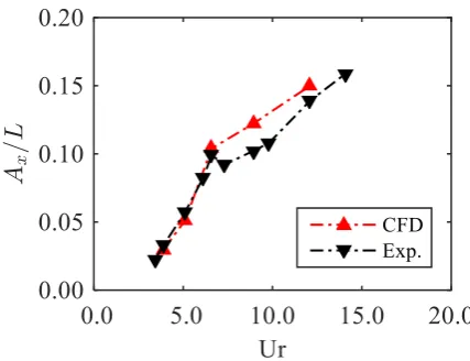
Fig. 17. Non-dimensional in-line characteristic amplitudes (Ax⁄L), the Ur is defined based on the
385
[image:23.595.184.398.348.512.2]24 387
Fig. 18. Non-dimensional yaw characteristic amplitudes, the Ur is defined based on the natural period 388
of the yaw motion. 389
Fig. 16, Fig. 17 and Fig. 18 present the non-dimensional transverse, in-line and yaw motion 390
amplitudes obtained from the numerical simulations and the experimental measurements. In each 391
case, the numerical predictions show a good agreement with the experimental results. However, at 392
low Ur values, the numerical simulation predicts a slightly larger transverse response than the 393
experimental data. An analysis of the error will be given in the following 3.3.3. Force analysis section 394
together with the added mass analysis. From the non-dimensional transverse characteristic amplitude 395
in Fig. 16, the “lock-in” phenomenon can be clearly seen occurring in a reduced velocity range from 5 396
to 9. The transverse motion increased rapidly from the “pre lock-in” region to the “lock-in” region, 397
and then sharply declines from the “lock-in” region to the following “post lock-in” region. The peak 398
point for the transverse motion is at Ur = 6.6. 399
3.3.3. Force analysis 400
In order to study the fluctuation forces responsible for VIM, the lift and drag forces and the related 401
coefficients are further analysed. Fig. 19 and Fig. 20 show the mean drag force coefficient (C̅D) and 402
the root mean square lift force coefficient (CLrms) respectively as a function of the reduced velocity
403
25 the experimental measurements. However, there is a discrepancy between the numerical predictions 405
and the experimental data at low reduced velocity levels for the root mean square lift force coefficient, 406
similar to the trend observed in the non-dimensional transverse characteristic amplitudes in Fig. 16. 407
408
Fig. 19. Mean drag coefficient (C̅D) from the numerical and experimental results on the VIM model, 409
the Ur is defined based on the natural period of the transverse motion. 410
[image:25.595.185.397.171.336.2]411
Fig. 20. Root mean square lift coefficient (CLrms) from the numerical and experimental results on the
412
VIM model, the Ur is defined based on the natural period of the transverse motion. 413
To further examine the differences, a virtual variable so-called added mass coefficient (Ca) has been 414
26 measurements. Similar to the discussions made by Sarpkaya (2004) in their vortex-induced vibrations 416
study, Zhang et al. (2014) introduced this variable into a Spar VIM investigation. In their work, the 417
added mass coefficient (Ca) is estimated by the equations proposed by Vikestad et al. (2000) as
418
follows: 419
Ca= mρ∆a, (8)
420
Ca=- 2
nTρ∆(√2rms(ÿ))2∫ Fyÿdt t+nT
t , (9)
421
where n is an integer number of oscillation periods, nT is the time length, ρ is the fresh water density, 422
∆ is the displacement of the structure, Fy is the cross-flow component of the total hydrodynamic force 423
on the structure and y is the transverse displacement of the motion. 424
[image:26.595.185.400.401.559.2]425
Fig. 21. Added mass coefficient (Ca) of the VIM model from the numerical predictions and the
426
experiments, the Ur is defined based on the natural period of the transverse motion. 427
Fig. 21 shows the comparison of the added mass coefficients (Ca) obtained from the numerical 428
calculations and the experiments. The numerical prediction shows a decreasing trend similar to that 429
reported in an earlier study by Zhang et al. (2014). This trend is also the same as the results from the 430
studies conducted by Sarpkaya (2004). However, the added mass coefficient (Ca) obtained from the
27 experimental measurements at low reduced velocity range are significantly different to those from the 432
present numerical predictions. A distinct feature shown in Fig. 21 is that the added mass coefficient 433
from experiments is much smaller at very low Ur and trends to increase initially and then decrease 434
rapidly with the increases of the reduced velocity. The apparent discrepancy between the numerical 435
and experimental results at low reduced velocities is likely to be caused by the experimental data. 436
There are a few possibilities that could cause the error. Firstly, the towing speed during the 437
experiment is extremely low for an equivalent low reduced velocity (for example, 0.073m/s for 438
reduced velocity at Ur = 3.4), and the whole system mechanical friction may affect the experimental 439
measurements at such a low towing speed; secondly, the influence of the mooring line settings may 440
also affect the experimental measurements, because the theoretically linear springs set in numerical 441
simulations are ideal springs and the mooring lines in the experimental set-up may not be arranged as 442
symmetrically as in the numerical simulations. Due to these factors, the numerical results may be 443
more reliable and accurate than the experimental data in the low reduced velocity range. 444
Similar to the motion observation, the “lock-in” phenomenon can also be seen in Fig. 19 and Fig. 20. 445
However, it is noted that the “lock-in” phenomenon in the force domain is seen to occur slightly 446
earlier than in the transverse motion domain, as also observed by Gonçalves et al. (2012) in their 447
experiments. The peak point for the drag and lift force coefficients in the present study are at Ur = 5.1 448
while the peak point for the transverse motion is at Ur = 6.6. 449
Both the transverse motion time histories and the lift force coefficient time histories are transferred 450
from the time domain to the frequency domain by using the Fast Fourier transform (FFT) in order to 451
study the “lock-in” phenomenon. The frequency domain results are shown in Fig. 22 to Fig. 26, 452
inclusive the “pre lock-in”, “lock-in” and “post lock-in” regions. The transverse motion frequency and 453
vortex shedding frequency are both close to the transverse natural frequency in still water at the “pre 454
lock-in” and “lock-in” regions. The oscillation and vortex shedding frequency are shown increasing 455
with the increase in reduced velocity. When the “post lock-in” started, the oscillation frequency and 456
28 can be seen in Fig. 25. For the highest reduced velocity case at Ur = 12.1, Fig. 26 shows multiple 458
peak frequencies appearing in the frequency domain. 459
As can be seen in Fig. 22 to Fig. 25, the agreement between the numerical predictions and the 460
experimental measurements for both transverse motions and the lift force coefficients are reasonably 461
well. It is seen that in Fig. 26, however, at “Ur = 12.1”, the agreement is less well especially the 462
magnitudes of motion and force coefficient though the dominant frequencies were still predicted 463
accurately. It is noted that, at such a high reduced velocity (Ur = 12.1) far beyond the “lock-in” region 464
(approx. Ur = 6.6), the magnitudes of the transverse motion and lift force coefficient are much 465
smaller, thus, the relatively larger discrepancies appeared in Fig. 26. 466
Compared to Fig. 24 with Ur = 6.6, Fig. 23 shows that the oscillation frequency and vortex shedding 467
frequency are closer to the transverse natural frequency at Ur = 5.1, where the values of the peak drag 468
and lift force coefficients appear. Furthermore, the added mass may also contribute to the earlier peak 469
drag and lift force occurrence. Since the added mass keeps decreasing with the reduced velocity 470
increasing, the force domain and the motion domain may have a hysteresis phenomenon which 471
requires further studies. 472
[image:28.595.68.512.509.680.2]473
Fig. 22. FFT of the transverse motions and the lift force coefficients at Ur = 3.9, (a) transverse 474
29 476
Fig. 23. FFT of the transverse motions and the lift force coefficients at Ur = 5.1, (a) transverse 477
motion; (b) lift force coefficient. 478
479
Fig. 24. FFT of the transverse motions and the lift force coefficients at Ur = 6.6, (a) transverse 480
[image:29.595.64.514.343.516.2]30 482
Fig. 25. FFT of the transverse motions and the lift force coefficients at Ur = 8.9, (a) transverse 483
motion; (b) lift force coefficient. 484
485
Fig. 26. FFT of the transverse motions and the lift force coefficients at Ur = 12.1, (a) transverse 486
motion; (b) lift force coefficient. 487
To examine the complex fluid mechanisms on the structure and the corresponding motion driven parts 488
of the structure, the drag and lift force coefficients on different structure members of the DDS are 489
further calculated and analysed. 490
Unlike the stationary model, the drag and lift force coefficients are changed when the reduced 491
[image:30.595.67.515.344.517.2]31 (Column 1), the portside column (Column 2) and the starboard side column (Column 4) are excited by 493
the “lock-in” phenomenon. The pontoons are less excited compared to the three aforementioned 494
columns. However, the drag force coefficient on the downstream column (Column 3) is decreasing 495
while coefficients for the other members experiencing increasing trends and only recovers when “post 496
lock-in” phase starts. The drag force coefficient on the downstream column is also much smaller than 497
that for other members of the structure. On the other hand, the lift force coefficient (CLrms) on the 498
downstream column, the portside and starboard side columns, and on the pontoons, are all excited by 499
the “lock-in” phenomenon. At this time, the leading upstream column shows a different trend. The lift 500
force coefficient on the upstream column is seen to decrease while an increasing trend is observed for 501
the other components, and conversely starts to recover as the other components begin to decrease. 502
This is due to the wake region changing behind each of the columns. Further details will be discussed 503
in the 3.3.4. Flow pattern section. 504
[image:31.595.184.413.400.565.2]505
32 507
Fig. 28. Root mean square lift coefficients (CLrms) on each member of the DDS from the VIM model. 508
The drag and lift forces on the structure are nearly symmetric except the lift force coefficient 509
distribution at Ur = 5.1. Due to the results being based on the motion-coupled simulations, the rigid 510
body motion also needs to be included in the analysis. With this aim, the work done by each member 511
of the structure during the stabilized VIM time is calculated and the results are presented in Fig. 29. 512
The work done is calculated using the following equations: 513
W=F∙S, (10) 514
where F is the total drag and lift force of the structure and S is the displacement of the structure 515
motion. 516
33 Fig. 29. Work done by each member of the DDS on VIM model.
518
In Fig. 29, the symmetrical characteristics can be clearly identified, and the following features can be 519
observed: 520
1) The pontoon reduces the VIM response throughout the reduced velocity range. Thus, adding 521
on the pontoon into the overall structure is a good design for restraining VIM responses. 522
2) The three upstream columns excite VIM responses. Further, the portside and starboard side 523
columns excite VIM responses in the “lock-in” region and trend to resist VIM responses in 524
the “post lock-in” region. 525
3) The downstream column shows a different trend compared to the portside and starboard side 526
columns; the work done by the downstream column drops initially and then recovers. 527
3.3.4. Flow pattern 528
In order to have a general visual appreciation of the vortex shedding patterns, the vorticity contours 529
are plotted in Fig. 31 to Fig. 40. Two dimensional variables (dimensional vorticity and non-530
dimensional spanwise vorticity) are used to describe the vorticity in the current study. 531
non-dimensional vorticity = ωD/U, (11) 532
ω = √ω⃑⃑ x2+⃑⃑ ωy2+ω⃑⃑ z2, (12)
533
non-dimensional spanwise vorticity = ω⃑⃑ zD/U, (13)
534
where, ω is the vorticity magnitude, ω⃑⃑ x, ω⃑⃑ y and ω⃑⃑ z are the x, y, and z components of the vorticity, D is
535
34 For convenience in describing the vortex development processes, four regions are defined around the 537
column, named as NW (Northwest), NE (Northeast), SW (Southwest) and SE (Southeast) (see Fig. 538
30). The vortices shed from each side of the column are denoted in chronological order of genesis 539
(e.g., A1, A2 …) from the upper side of Column 1, see Table 6. 540
[image:34.595.184.412.199.360.2]541
Fig. 30. Definition of the regions around the individual column. 542
Table 6. The chronological order of vortices genesis for each column. 543
Column Shear layer Vortex street
1 Upper A1, A2 …
Lower B1, B2 …
2 Upper C1, C2 …
Lower D1, D2 …
3 Upper E1, E2 …
Lower F1, F2 …
4 Upper G1, G2 …
[image:34.595.136.460.486.607.2]35 544
Fig. 31. A time series of the non-dimensional spanwise vorticity (ω⃑⃑ zD/U) contours around the DDS at
545
36 the non-dimensional transverse motion (y/L) time history (F); the red arrow is the DDS transverse 547
velocity direction. 548
37 Fig. 32. A time series of the non-dimensional vorticity (ωD/U) contours around the DDS at middle 550
draft showing the instantaneous flow fields around the DDS at Ur = 3.9 (A, B, C, D, E) and the non-551
dimensional motion trajectory (F); the red arrow is the DDS transverse velocity direction. 552
Fig. 31 presents the non-dimensional spanwise vorticity (ω⃑⃑ zD/U) contours at Ur = 3.9. As can be
553
seen, the vortices shed from the upstream column (Column 1) directly impinge on the downstream 554
column (Column 3) and then join into the downstream column’s weak region. The vortex street can be 555
clearly found behind the upstream column where the “2S” type shedding occurs. Additionally, the 556
vortices shed from the portside and starboard side columns (Column 2 and 4) also impinge on the 557
downstream column, which are red circled in Fig. 32(B). These vortex patterns are not visible in the 558
spanwise vorticity contour (Fig. 31) indicating that there are three-dimensional effects on the flow 559
characteristics especially on the side columns’ wake region and the flow region in front of the 560
38 562
Fig. 33. A time series of the non-dimensional spanwise vorticity (ω⃑⃑ zD/U) contours around the DDS at
563
39 the non-dimensional transverse motion (y/L) time history(F); the red arrow is the DDS transverse 565
velocity direction. 566
40 Fig. 34. A time series of the non-dimensional vorticity (ωD/U) contours around the DDS at middle 568
draft showing the instantaneous flow fields around the DDS at Ur = 5.1 (A, B, C, D, E) and the non-569
dimensional motion trajectory (F); the red arrow is the DDS transverse velocity direction. 570
With the increase of the Ur, in the “lock-in” region, the flow patterns are changed. When Ur = 5.1, the 571
structure oscillation frequency is close to the natural frequency of the structure in still water. As the 572
result of the resonance developing, the motion starts to amplify and the flow patterns are changed 573
significantly. Vortex streets only appear on the opposite of the transverse velocity direction (see Fig. 574
33 and Fig. 34). The vortices shed from the upstream column (Column 1) where the “P+S” type 575
shedding occurred periodically and symmetrically impinge on the portside and starboard side 576
(Column 2 and 4). Respectively, the vortices generated by the upstream column impinge on the NW 577
face of the portside column (Column 2) and the SW face of the starboard side column (Column 4). 578
Only one strong vortex will form on the opposite side to the transverse velocity direction behind 579
portside and starboard side columns (see “D1, H1, G1” in Fig. 33). Also, the vortices shed from the 580
side columns impinge on the downstream column (Column 3). As a result, there is no clear vortex 581
street behind the downstream column. Small vortices in piece can be seen in the downstream of 582
41 584
Fig. 35. A time series of the non-dimensional spanwise vorticity (ω⃑⃑ zD/U) contours around the DDS at
585
42 the non-dimensional transverse motion (y/L) time history (F); the red arrow is the DDS transverse 587
velocity direction. 588
43 Fig. 36. A time series of the non-dimensional vorticity (ωD/U) contours around the DDS at middle 590
draft showing the instantaneous flow fields around the DDS at Ur = 6.6 (A, B, C, D, E) and the non-591
dimensional motion trajectory (F); the red arrow is the DDS transverse velocity direction. 592
With a further slight increase of the Ur, the transverse motion keeps amplifying. However, the lift 593
force coefficient reduces (see Fig. 16 and Fig. 20). This hysteresis phenomenon can be explained by 594
Fig. 35. As the transverse motion is amplified, after impinging on the starboard side column (Column 595
4), the vortices that are shed from the upstream column (Column 1) move back to impinge on the 596
portside column (Column 2). This can be seen by following the trajectory of the vortices “B1”. 597
Additionally, the vortices like “B1” affect the vortices detached from the upper side of Column 2 and 598
lower side of Column 4. As can be seen in Fig. 35(B) (red circled), two different clockwise vortices 599
are mixed together on the SE face of the starboard side column. The mixing of the vortices can 600
decrease the lift force on the structure. This is one of the reasons that makes the lift force coefficient 601
on the structures drops while the transverse motion increases. By comparing the differences between 602
Fig. 33 and Fig. 35, there is another factor which may contribute to the hysteresis phenomenon. In 603
Fig. 35, it is seen that strong vortices are detached from both portside and starboard side at same time. 604
While in Fig. 33, only one strong vortex will form on the opposite side to the transverse velocity 605
direction behind portside and starboard side columns. The differences of the flow characteristics 606
shown in Fig. 33 and Fig. 35 lead to the peak point in the force domain occurs slightly earlier than 607
44 609
Fig. 37. A time series of the non-dimensional spanwise vorticity (ω⃑⃑ zD/U) contours around the DDS at
610
45 the non-dimensional transverse motion (y/L) time history (F); the red arrow is the DDS transverse 612
velocity direction. 613
46 Fig. 38. A time series of the non-dimensional vorticity (ωD/U) contours around the DDS at middle 615
draft showing the instantaneous flow fields around the DDS at Ur = 8.9 (A, B, C, D, E) and the non-616
dimensional motion trajectory (F); the red arrow is the DDS transverse velocity direction. 617
47 Fig. 39. A time series of the non-dimensional spanwise vorticity (ω⃑⃑ zD/U) contours around the DDS at
619
middle draft showing the instantaneous flow fields around the DDS at Ur = 12.1 (A, B, C, D, E) and 620
the non-dimensional transverse motion (y/L) time history (F); the red arrow is the DDS transverse 621
48 623
Fig. 40. A time series of the non-dimensional vorticity (ωD/U) contours around the DDS at middle 624
draft showing the instantaneous flow fields around the DDS at Ur = 12.1 (A, B, C, D, E) and the non-625
49 When the reduced velocity reaches the “post lock-in” region, the vortices shed from the upstream 627
column (Column 1) no longer impinge on the incidence flow faces of the portside and starboard side 628
columns (Column 2 and 4). Instead, the vortices are seen to join the weak region of the portside and 629
starboard side (see Fig. 37 to Fig. 40). The vortex street behind the Column 1, 2 and 4 can be clearly 630
seen. In addition, it can be seen in Fig. 40(A) that parts of these vortices (red circled) do act on the 631
incidence flow face of the downstream column (Column 3). As the vortices shed from the upstream 632
column do not impinge on the portside and starboard side columns, the lift force coefficient and the 633
transverse motion decrease and then remain a stable value in the measurement range of the “post lock-634
in” region in the present study. 635
4.
Conclusions
636
This paper presented a numerical study on the forces and VIM of a deep-draft semi-submersible. 637
Two different models were considered, i.e., a stationary model and a VIM model. For the stationary 638
model, the drag and lift force distributions on each structural member of the DDS are discussed and 639
followed by the flow pattern analyses. The vortex interactions between each column are presented to 640
explain the hysteresis phenomenon. The numerical model predicts forces well compared to the 641
experimental results. For the VIM model, the motion and force on the whole structures are analysed, 642
and the “pre lock-in”, “lock-in” and “post lock-in” phases can be accurately predicted in the present 643
study. It is revealed that the discrepancies in the drag and lift forces between the numerical predictions 644
and the experimental measurements at low reduced velocity is likely to be caused by the uncertainty 645
in the experimental measurements at very low towing speed in the experiments. It is demonstrated 646
that the numerical approach is a good way to predict the VIM responses at the low reduce velocity 647
range. 648
Analysis of the drag and lift force coefficients on and the work done by different members of the DDS 649
revealed that the portside and starboard side columns are the key structure members responsible for 650
50 The present numerical study confirmed the hysteresis phenomenon - the peak lift force occurs slightly 652
earlier than the peak transverse motion. By examining the flow patterns at the time instantaneous near 653
the peak response, it is revealed that the hysteresis phenomenon between the force and motion is 654
mainly due to the vortices shed from the upstream column move back to impinge on one of the side 655
columns after impinging on the other side column and the symmetrical strong vortices which shed 656
from the side columns. 657
This study focuses on the 45 degree flow incidence on the DDS, more incidences should be 658
considered and examined in order to obtain a more generalized understanding on VIM of a multi-659
column structures. 660
Acknowledgment
661
The authors would like to acknowledge the support of Newton Fund of Royal Academy of 662
Engineering UK (NRCP/1415/211) and the National Natural Science Foundation of China (Grant No. 663
51279104). This work made use of the facilities of N8 HPC Centre of Excellence, provided and 664
funded by the N8 consortium and EPSRC (Grant No. EP/K000225/1). 665
References
666
Antony, A., Vinayan, V., Halkyard, J., Kim, S.-J., Holmes, S., Spernjak, D., 2015. A CFD Based 667
Analysis of the Vortex Induced Motion of Deep-Draft Semisubmersibles, The Twenty-fifth 668
International Offshore and Polar Engineering Conference. International Society of Offshore 669
and Polar Engineers. 670
Antony, A., Vinayan, V., Madhavan, S., Parambath, A., Halkyard, J., Sterenborg, J., Holmes, S., 671
Spernjak, D., Kim, S.J., Head, W., 2016. VIM Model Test of Deep Draft Semisubmersibles 672
Including Effects of Damping, Offshore Technology Conference. Offshore Technology 673
Conference. 674
51 Celik, I.B., Ghia, U., Roache, P.J., 2008. Procedure for estimation and reporting of uncertainty due to 676
discretization in CFD applications. Journal of fluids Engineering-Transactions of the ASME 677
130 (7). 678
Chen, J.M., Chiou, C.-C., 1997. Flow past a blunt flat plate subjected to the disturbance of incident 679
vortex street. Journal of Wind Engineering and Industrial Aerodynamics 66 (3), 179-196. 680
Fujarra, A.L.C., Rosetti, G.F., de Wilde, J., Gonçalves, R.T., 2012. State-of-art on vortex-induced 681
motion: a comprehensive survey after more than one decade of experimental investigation, 682
ASME 2012 31st International Conference on Ocean, Offshore and Arctic Engineering. 683
American Society of Mechanical Engineers, pp. 561-582. 684
Gonçalves, R.T., Fujarra, A.L.C., Rosetti, G.F., Kogishi, A.M., Koop, A., 2015. Effects of Column 685
Designs on the VIM Response of Deep-Draft Semi-Submersible Platforms, The Twenty-fifth 686
International Offshore and Polar Engineering Conference. International Society of Offshore 687
and Polar Engineers. 688
Gonçalves, R.T., Rosetti, G.F., Fujarra, A.L.C., Oliveira, A.C., 2012. Experimental study on vortex-689
induced motions of a semi-submersible platform with four square columns, Part I: Effects of 690
current incidence angle and hull appendages. Ocean Engineering 54, 150-169. 691
Gonçalves, R.T., Rosetti, G.F., Fujarra, A.L.C., Oliveira, A.C., 2013. Experimental study on vortex-692
induced motions of a semi-submersible platform with four square columns, Part II: Effects of 693
surface waves, external damping and draft condition. Ocean Engineering 62, 10-24. 694
Hong, Y., Choi, Y., Lee, J., Kim, Y., 2008. Vortex-induced motion of a deep-draft semi-submersible 695
in current and waves, The Eighteenth International Offshore and Polar Engineering 696
Conference. International Society of Offshore and Polar Engineers. 697
Kokkinis, T., Sandström, R.E., Jones, H.T., Thompson, H.M., Greiner, W.L., 2004. Development of a 698
Stepped Line Tensioning Solution for Mitigating VIM Effects in Loop Eddy Currents for the 699
Genesis Spar, ASME 2004 23rd International Conference on Offshore Mechanics and Arctic 700
52 Koop, A., Rijken, O., Vaz, G., Maximiano, A., Rosetti, G., 2016. CFD Investigation on Scale and 702
Damping Effects for Vortex Induced Motions of a Semi-Submersible Floater, Offshore 703
Technology Conference. Offshore Technology Conference. 704
Lam, K., Li, J.Y., So, R.M.C., 2003b. Force coefficients and Strouhal numbers of four cylinders in 705
cross flow. Journal of Fluids and structures 18 (3), 305-324. 706
Lee, S.-K., Chien, H.-P., Gu, H., 2014. CFD Study of Deep Draft SemiSubmersible VIM, Offshore 707
Technology Conference-Asia. Offshore Technology Conference. 708
Lefevre, C., Constantinides, Y., Kim, J.W., Henneke, M., Gordon, R., Jang, H., Wu, G., 2013. 709
Guidelines for CFD Simulations of Spar VIM, ASME 2013 32nd International Conference on 710
Ocean, Offshore and Arctic Engineering. American Society of Mechanical Engineers, pp. 711
V007T008A019-V007T008A019. 712
Liang, Y., Tao, L., Xiao, L., Liu, M., 2016. Experimental and Numerical Study on Vortex-Induced 713
Motions of a Deep-Draft Semi-Submersible, Manuscript submitted for publication. 714
Liu, C.-H., Chen, J.M., 2002. Observations of hysteresis in flow around two square cylinders in a 715
tandem arrangement. Journal of Wind Engineering and Industrial Aerodynamics 90 (9), 1019-716
1050. 717
Liu, M., Xiao, L., Lyu, H., Tao, L., 2015. Numerical Analysis of Pontoon Effect on Flow-Induced 718
Forces of the Deep Draft Semisubmersible in a Cross-Flow, ASME 2015 34th International 719
Conference on Ocean, Offshore and Arctic Engineering. American Society of Mechanical 720
Engineers, pp. V001T001A030-V001T001A030. 721
Ljungkrona, L., Norberg, C.H., Sunden, B., 1991. Free-stream turbulence and tube spacing effects on 722
surface pressure fluctuations for two tubes in an in-line arrangement. Journal of Fluids and 723
structures 5 (6), 701-727. 724
Ma, W., Wu, G., Thompson, H., Prislin, I., Maroju, S., 2013. Vortex induced motions of a column 725
stabilized floater, Proceedings of the DOT International Conference, pp. 22-24. 726
Magee, A., Sheikh, R., Guan, K.Y.H., Choo, J.T.H., Malik, A.M.A., Ghani, M.P.A., Abyn, H., 2011. 727
53 Conference on Ocean, Offshore and Arctic Engineering. American Society of Mechanical 729
Engineers, pp. 127-136. 730
Rijken, O., Leverette, S., 2008. Experimental Study into Vortex Induced Motion Response of Semi 731
Submersibles with Square Columns, ASME 2008 27th International Conference on Offshore 732
Mechanics and Arctic Engineering. American Society of Mechanical Engineers, pp. 263-276. 733
Rijken, O., Leverette, S., 2009. Field measurements of vortex induced motions of a deep draft 734
semisubmersible, ASME 2009 28th International Conference on Ocean, Offshore and Arctic 735
Engineering. American Society of Mechanical Engineers, pp. 739-746. 736
Rijken, O., Schuurmans, S., Leverette, S., 2011. Experimental investigations into the influences of 737
SCRs and appurtenances on DeepDraft Semisubmersible Vortex Induced Motion response, 738
Proceedings of the 30th International Conference on Ocean, Offshore and Arctic Engineering, 739
Rotterdam, The Netherlands, OMAE2011-49365. 740
Sarpkaya, T., 2004. A critical review of the intrinsic nature of vortex-induced vibrations. Journal of 741
Fluids and structures 19 (4), 389-447. 742
Schewe, G., 1983. On the force fluctuations acting on a circular cylinder in crossflow from subcritical 743
up to transcritical Reynolds numbers. Journal of Fluid Mechanics 133, 265-285. 744
Shur, M.L., Spalart, P.R., Strelets, M.K., Travin, A.K., 2008. A hybrid RANS-LES approach with 745
delayed-DES and wall-modelled LES capabilities. International Journal of Heat and Fluid 746
Flow 29 (6), 1638-1649. 747
Spalart, P.R., Jou, W.H., Strelets, M., Allmaras, S.R., 1997. Comments on the feasibility of LES for 748
wings, and on a hybrid RANS/LES approach. Advances in DNS/LES 1, 4-8. 749
Tan, J.H.C., Magee, A., Kim, J.W., Teng, Y.J., Zukni, N.A., 2013. CFD Simulation for Vortex 750
Induced Motions of a Multi-Column Floating Platform, ASME 2013 32nd International 751
Conference on Ocean, Offshore and Arctic Engineering. American Society of Mechanical 752
Engineers, pp. V007T008A066-V007T008A066. 753
Vikestad, K., Vandiver, J.K., Larsen, C.M., 2000. Added mass and oscillation frequency for a circular 754
cylinder subjected to vortex-induced vibrations and external disturbance. Journal of Fluids 755
54 Vinayan, V., Antony, A., Halkyard, J., Kim, S.-J., Holmes, S., Spernjak, D., 2015. Vortex-Induced 757
Motion of Deep-Draft Semisubmersibles: A CFD-Based Parametric Study, ASME 2015 34th 758
International Conference on Ocean, Offshore and Arctic Engineering. American Society of 759
Mechanical Engineers, pp. V002T008A003-V002T008A003. 760
Waals, O.J., Phadke, A.C., Bultema, S., 2007. Flow Induced Motions on Multi Column Floaters, 761
ASME 2007 26th International Conference on Offshore Mechanics and Arctic Engineering. 762
American Society of Mechanical Engineers, pp. 669-678. 763
Zhang, H., Yang, J., Xiao, L., Lu, H., 2014. Study on added mass coefficient and oscillation 764
frequency for a Truss Spar subjected to Vortex-Induced Motions. Ships and Offshore 765
Structures 9 (1), 54-63. 766
55
List of Tables
769
Table 1. Main characteristics of the DDS unit (The model I is the stationary model which presents 770
scale ratio as 1:128, and the model II is the VIM model which presents scale ratio as 1:64). 771
Table 2. Calculations of discretization error (Celik et al., 2008); GCI index represents the numerical 772
uncertainty. 773
Table 3. Summary of the various studies on VIM of the multiple square section shaped columns 774
structures. 775
Table 4. The resulting force coefficient values C̅D, CLrms and St for the flow over a stationary DDS.
776
Table 5. Natural periods of the motions in calm water. 777
Table 6. The chronological order of vortices genesis for each column. 778