doi: 10.3389/fmars.2019.00035
Edited by:
Amos Tiereyangn Kabo-Bah, University of Energy and Natural Resources, Ghana
Reviewed by:
Antonio Cobelo-Garcia, Spanish National Research Council (CSIC), Spain Miguel Angel Huerta-Diaz, Universidad Autónoma de Baja California, Mexico
*Correspondence:
Maxime M. Grand [email protected]
Specialty section:
This article was submitted to Marine Biogeochemistry, a section of the journal Frontiers in Marine Science
Received:14 November 2018
Accepted:22 January 2019
Published:21 February 2019
Citation:
Grand MM, Laes-Huon A, Fietz S, Resing JA, Obata H, Luther GW III, Tagliabue A, Achterberg EP, Middag R, Tovar-Sánchez A and Bowie AR (2019) Developing Autonomous Observing Systems for Micronutrient Trace Metals. Front. Mar. Sci. 6:35. doi: 10.3389/fmars.2019.00035
Developing Autonomous Observing
Systems for Micronutrient Trace
Metals
Maxime M. Grand1* , Agathe Laes-Huon2, Susanne Fietz3, Joseph A. Resing4,
Hajime Obata5, George W. Luther III6, Alessandro Tagliabue7, Eric P. Achterberg8,
Rob Middag9, Antonio Tovar-Sánchez10and Andrew R. Bowie11
1Moss Landing Marine Laboratories, Moss Landing, CA, United States,2Laboratoire Détection Capteurs et Mesures, Unité de Recherches et Développements Technologiques, Ifremer, France,3Department of Earth Sciences, Stellenbosch University, Stellenbosch, South Africa,4Joint Institute for the Study of the Atmosphere and Ocean, University of Washington and NOAA-Pacific Marine Environmental Laboratory, Seattle, WA, United States,5Atmosphere and Ocean Research Institute, The University of Tokyo, Chiba, Japan,6School of Marine Science and Policy, University of Delaware, Lewes, DE, United States,7School of Environmental Sciences, University of Liverpool, Liverpool, United Kingdom,8GEOMAR Helmholtz Centre for Ocean Research Kiel, Kiel, Germany,9Department of Ocean Systems (OCS), NIOZ Royal Netherlands Institute for Sea Research, and Utrecht University, Texel, Netherlands,10ICMAN – Institute of Marine Science of Andalusia (CSIC), Campus Universitario Río San Pedro, Cádiz, Spain,11Institute for Marine and Antarctic Studies and Antarctic Climate and Ecosystems Cooperative Research Centre, University of Tasmania, Hobart, TAS, Australia
Trace metal micronutrients are integral to the functioning of marine ecosystems and the export of particulate carbon to the deep ocean. Although much progress has been made in mapping the distributions of metal micronutrients throughout the ocean over the last 30 years, there remain information gaps, most notable during seasonal transitions and in remote regions. The next challenge is to developin situsensing technologies necessary to capture the spatial and temporal variabilities of micronutrients characterized with short residence times, highly variable source terms, and sub-nanomolar concentrations in open ocean settings. Such an effort will allow investigation of the biogeochemical processes at the necessary resolution to constrain fluxes, residence times, and the biological and chemical responses to varying metal inputs in a changing ocean. Here, we discuss the current state of the art and analytical challenges associated with metal micronutrient determinations and highlight existing and emerging technologies, namely
technologies to in situ applications; and (4) develop a community-led standardized protocol to demonstrate the endurance and comparability of in situ sensor data with established techniques. Such a vision will be best served through ongoing collaborations between trace metal geochemists, analytical chemists, the engineering community, and commercial partners, which will accelerate the delivery of new technologies for in situ
metal sensing in the decade following OceanObs’19.
Keywords: trace metals, micronutrients,in situchemical analyzers,in situsensors, GEOTRACES, OceanObs’19, ocean observing time series
INTRODUCTION
Bioactive micronutrient metals are essential for cell functions and mediate vital biochemical reactions by acting as cofactors in many enzymes and as centers to stabilize enzymes and protein structures (Sunda, 2012). These micronutrients – cobalt (Co), copper (Cu), iron (Fe), manganese (Mn), nickel (Ni), zinc (Zn), and to a lesser extent cadmium (Cd) – are thus required for marine life, but can hinder cell growth at higher concentrations (e.g., through anthropogenic inputs in coastal regions). Since phytoplankton species have different cellular metal requirements (e.g., Ho et al., 2003; Twining and Baines, 2013), the supply and concentration of metal micronutrients in the ocean affects the growth and turnover rate of phytoplankton, and modulates phytoplankton species composition. The distribution of metal micronutrients ultimately influences the productivity of entire food webs and the rate of particulate carbon export to the deep ocean.
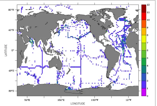
Over the past 30 years, from the pioneering work of John Martin on Fe limitation (Martin and Fitzwater, 1988;Martin and Gordon, 1988) to the ongoing GEOTRACES program that is mapping the distributions and investigating the biogeochemistry of trace elements and their isotopes throughout the ocean (Schlitzer et al., 2018), the database of discrete observations for Fe and other bioactive trace metals has grown by three orders of magnitude and encompasses observations in all ocean basins (Tagliabue et al., 2017 and references therein). These sampling efforts have greatly improved our understanding of micronutrient cycling, but are not sufficient to constrain the key processes underpinning metal micronutrient cycling and associated biological responses. For instance, Fe currently has the highest spatial and temporal observational coverage relative to all other metal micronutrients; however, Figure 1
illustrates that even for Fe there remains large spatial gaps along with poor temporal resolution. Ship-based sampling campaigns only provide a one-time snapshot of distributions in logistically accessible regions. However, micronutrients are generally characterized by short residence times and highly variable inputs in space and time (Tagliabue et al., 2017 and references therein). As a result, the external fluxes, removal rates, internal cycling, and residence times of bioactive trace metals remain poorly constrained and their spatial and temporal variability incompletely characterized, particularly in remote regions of the oceans. This lack of understanding cascades into an incomplete representation of ocean Fe cycling in the global
models used to project the impacts of change in Fe-limited regions (Tagliabue et al., 2016).
Metal micronutrients enter the ocean through a variety of highly episodic sources, including atmospheric deposition, sediment–water exchange at the land–ocean interface and intermittent venting from hydrothermal vents, which supply both metals and metal-binding ligands to the deep ocean. Metal concentrations have been observed to vary from days to months as a result of the passage of mesoscale eddies (Fitzsimmons et al., 2015), changes in mixed-layer depth via wind-driven mixing (Nishioka et al., 2007, 2011), coastal upwelling (Elrod et al., 2008), and seasonal fluctuations in dust and associated wet deposition (Boyle et al., 2005;Sedwick et al., 2005). The biological response to changing metal micronutrient distributions is also highly dynamic, ranging from fast changes in cellular stoichiometry (Twining et al., 2010) to impacts on growth rates. Experimental evidence shows that enhanced inputs of metal micronutrients can either enhance (e.g., Fe, Coale et al., 1996) or inhibit (e.g., excessive Cu, Mann et al., 2002; Jordi et al., 2012) phytoplankton productivity on time scales of hours to weeks. In some coastal settings, metal availability and intracellular concentrations of domoic acid, a neurotoxin, appear to be tightly coupled (Maldonado et al., 2002), indicating an important role for metals in influencing the toxicity and occurrence of harmful algal blooms and the management response needed to mitigate impacts on local communities.
The short time-scale dynamics of micronutrient cycling are incompatible with discrete sampling approaches and require rapid and adaptivein situobservations to characterize episodic events and assess the biological implications of changing metal distributions. Developing the ability to obtain continuous, long-termin situtime-series for micronutrient metals is thus a pressing need in the field of trace metal biogeochemistry and such a development will improve model parameterizations of the key processes governing the distributions of micronutrients. Such work would better constrain metal fluxes and residence times, and improve our understanding of marine ecosystem dynamics following episodic events, as well as providing a baseline for detecting and predicting climate-driven changes. However, there are, at present, no micronutrient analyzers/sensors with analytical sensitivities suitable for open-ocean determinations of any of the micronutrient trace elements.
There are several regions in the ocean and specific episodic processes that would greatly benefit from high-resolutionin situ
FIGURE 1 |Published dissolved Fe observations as of 2018. To highlight the limited temporal resolution of current Fe observations, the color bar shows the number of unique months of sampling for dissolved Fe within a 2×2 degree box in the upper 100 m (n= 24,058 observations, datespan: 1978–2014, including all GEOTRACES IDP2017 measurements. The datespan refers to sample collection time and not publication of results). Except for a few repeat observations (e.g., Monterey Bay, HOTS, Arabian Sea, Ross Sea, Indian and Australian Sectors of the Southern Ocean, and North Atlantic), the majority of dissolved Fe observations consist of a one time “snapshot” (i.e., one unique month of sampling).
greatest benefit are either logistically difficult to reach during key seasonal transitions or need high-frequency observations to properly characterize sources and sinks of trace metals. The Southern Ocean, for example, where Fe plays a critical role in modulating productivity, lacks observations during key seasonal transitions (Tagliabue et al., 2012), which would provide important insights into the replenishment and depletion dynamics of Fe during the autumn–winter and winter–spring periods. Additionally, the Southern Ocean experiences variations in frontal positions and mixed-layer depths, affecting the recycling of micronutrients, leading to changes in plankton community structures (Deppeler and Davidson, 2017). An understanding of bioactive micronutrient dynamics would similarly be important in the subarctic North Pacific and Atlantic Oceans, which feature seasonal Fe limitation (Nishioka et al., 2007;Nielsdóttir et al., 2009;Ryan-Keogh et al., 2013;Westberry et al., 2016). Even the Arctic and Antarctic coasts represent important focus areas, where climate scenarios project enhanced continental runoff, and glacial and sea ice melting, which are expected to affect the distribution of metal micronutrients and
ligands and thereby impact primary productivity (Deppeler and Davidson, 2017; Rijkenberg et al., 2018). In situ ocean metal micronutrient observations at high latitudes during seasonal transitions would greatly improve our ability to monitor and predict the biological responses (across phytoplankton, bacteria, and archaea) to changes in micronutrient concentrations under a changing climate.
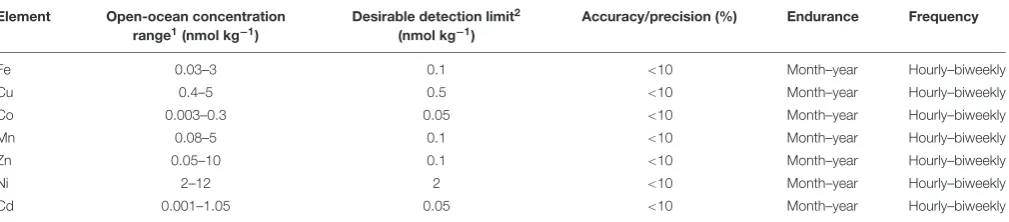
TABLE 1 |Ideal specifications of an autonomous observing system for metal micronutrients in the decade following OceanObs’19.
Element Open-ocean concentration range1(nmol kg−1)
Desirable detection limit2 (nmol kg−1)
Accuracy/precision (%) Endurance Frequency
Fe 0.03–3 0.1 <10 Month–year Hourly–biweekly
Cu 0.4–5 0.5 <10 Month–year Hourly–biweekly
Co 0.003–0.3 0.05 <10 Month–year Hourly–biweekly
Mn 0.08–5 0.1 <10 Month–year Hourly–biweekly
Zn 0.05–10 0.1 <10 Month–year Hourly–biweekly
Ni 2–12 2 <10 Month–year Hourly–biweekly
Cd 0.001–1.05 0.05 <10 Month–year Hourly–biweekly
The listed concentration and detection limits refer to total dissolved concentrations.1FromBruland et al. (2014).2Target detection limits refer to the minimum sensitivity that would be required to detect seasonal concentration changes in the euphotic zone.
and aboard autonomous surface sampling vehicles with a high payload. In the following, we seek to (1) describe the current state of the art and analytical challenges associated with micronutrient analysis; (2) highlight technologies amenable to
in situdeployment within the next decade, with a particular focus on techniques with potential for sub-nanomolar determinations of metals, including speciation; (3) identify key oceanic regions and processes where in situmonitoring would benefit pressing questions in trace metal biogeochemistry; and (4) develop a tangible roadmap for micronutrient metals sensing in the decade following OceanObs’19.
CURRENT ANALYTICAL STATE OF THE
ART: SHIPBOARD AND
IN SITU
Metal micronutrient analysis on discrete seawater samples is typically carried out using inductively coupled mass spectrometry (ICP-MS), Flow Injection Analysis (FIA), and anodic or adsorptive cathodic stripping voltammetry (ASV and AdCSV, respectively). These techniques feature detection limits suitable for open-ocean determinations at sub-nanomolar levels, but are not amenable to in situ deployment in their current state (Table 2).
ICP-MS
Inductively coupled mass spectrometry is generally regarded as the gold standard for metal micronutrient analysis in shore-based laboratories by virtue of the high precision and low detection limits (picomolar range) afforded by the technique, as well as convenience, since multi-elemental determinations can be performed on a single sample following preconcentration and matrix elimination (Milne et al., 2010;Biller and Bruland, 2012;
Lagerström et al., 2013;Minami et al., 2015;Rapp et al., 2017). However, current MS instrumentation requires complex sample pre-treatment, and is too resource demanding (gases, high-vacuum) or not sensitive enough (current miniature platforms) forin situdeployment in the foreseeable future.
FIA
Flow Injection Analysis manifolds couple preconcentration/ matrix elimination with absorbance, fluorescence, or chemiluminescence detection of individual elements (Fe,
Cu, Co, Mn, and Zn, Table 2), and have been very popular methods for metal micronutrient analysis onboard ships since the early 1990s (Elrod et al., 1991; Resing and Mottl, 1992;
Obata et al., 1993; Nowicki et al., 1994;Measures et al., 1995;
Bowie et al., 1998;Laës et al., 2007;Shelley et al., 2010;Klunder et al., 2011;Nishioka et al., 2011;Grand et al., 2015b;Rijkenberg et al., 2018). FIA systems are compact, portable, assembled using commercially available low-cost components, offer low detection limits (<0.1 nM), a rapid analytical throughput and can be connected to continuous underway sampling systems for near-real time surface mapping applications (e.g., Vink et al., 2000; Bowie et al., 2002). However, shipboard FIA systems are prone to drift (Floor et al., 2015), are characterized with high maintenance requirements, and consume large amounts of reagents and power, making them unsuitable for long and/or autonomous deployments (e.g., Johnson et al., 1986).
In situ chemical analyzers based on flow techniques have been developed for Fe and Mn (e.g.,Massoth, 1991;Chin et al., 1992;
Okamura et al., 2001;Sarradin et al., 2005;Vuillemin et al., 2009) and Cu (Holm et al., 2008), but the reported limits of detection of these submersible analyzers (Table 3), which were originally designed for monitoring metal dynamics in the vicinity of hydrothermal vent systems or in coastal regions, are inadequate for open-ocean determinations.
Voltammetry
TABLE 2 |State of the art figures of merit for lab and shipboard measurements on discrete samples.
Method Metal micronutrient LOD (nM) Species Pros and cons
HR ICP-MS1 Fe 0.02 Total dissolved High precision, low detection limits, multi-elemental
Cu 0.007 Total dissolved (UV irradiation) determinations. Not deployable.
Co 0.002 Total dissolved (UV irradiation)
Mn 0.007 Total dissolved
Zn 0.005 Total dissolved
Ni 0.026 Total dissolved
Cd 0.0006 Total dissolved
Shipboard FIA2 Fe 0.03 Total dissolved, Fe(II), Fe(III) Portable, low detection limits, easily assembled using Cu 0.03 Total dissolved, labile Cu(II) commercially available components. High reagent
Co 0.005 Total dissolved (UV irradiation) consumption and maintenance requirements.
Mn 0.03 Total dissolved
Zn 0.06 Total dissolved
Ni – No shipboard FIA method available
Cd – No shipboard FIA method available
AdCSV/ASV (Mn and Cd)3 Fe 0.1 Total dissolved (UV irradiation) Portable, low cost, low detection limits. Low reagent Cu 0.1 Total dissolved (UV irradiation) consumption, power and maintenance requirements.
Co 0.003 Total dissolved (UV irradiation)
Mn 0.2 Total dissolved (UV irradiation)
Zn 0.07 Total dissolved (UV irradiation)
Ni 0.1 Total dissolved (UV irradiation)
Cd 0.005 Total dissolved (UV irradiation)
1FromMilne et al. (2010).2LODs refer to typical detection limits that can be achieved using FIA, not individual analyst reports for each element.3FromAchterberg and
Braungardt (1999).
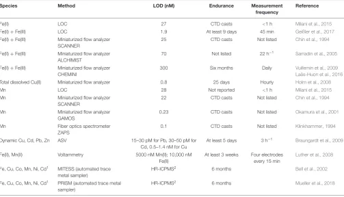
TABLE 3 |Figures of merit of currently availablein situsensors, analyzers, and autonomous samplers for dissolved metal micronutrients.
Species Method LOD (nM) Endurance Measurement
frequency
Reference
Fe(II) LOC 27 CTD casts <1 h Milani et al., 2015
Fe(II)+Fe(III) LOC 1.9 At least 9 days 45 min Geißler et al., 2017
Fe(II)+Fe(III) Miniaturized flow analyzer SCANNER
25 CTD casts Not listed Chin et al., 1994
Fe(II)+Fe(III) Miniaturized flow analyzer ALCHIMIST
70 Not listed 22 h−1 Sarradin et al., 2005
Fe(II)+Fe(III) Miniaturized flow analyzer CHEMINI
300 Six months Daily Vuillemin et al., 2009
Laës-Huon et al., 2016
Total dissolved Cu(II) Miniaturized flow analyzer 0.8 25 days Hourly Holm et al., 2008
Mn LOC 28 Not reported <1 h Milani et al., 2015
Mn Miniaturized flow analyzer
SCANNER
22 CTD casts Not listed Chin et al., 1994
Mn Miniaturized flow analyzer
GAMOS
0.23 CTD casts Not listed Okamura et al., 2001
Mn Fiber optics spectrometer
ZAPS
0.1 CTD casts Not listed Klinkhammer, 1994
Dynamic Cu, Cd, Pb, Zn ASV 15–30 pM for Pb, 30–50 pM for Cd, 0.5–1.4 nM for Cu
At least 5 days 3 h−1 Braungardt et al., 2009
Fe(II), Mn(II) Voltammetry 5000 nM Mn(II); 10,000 nM
Fe(II)
At least 3 weeks Four electrodes every 15 min
Luther et al., 2008
Fe, Cu, Co, Mn, Ni, Cd1 MITESS (automated trace metal sampler)
HR-ICPMS2 6 months Bell et al., 2002
Fe, Cu, Co, Mn, Ni, Cd1 PRISM (automated trace metal sampler)
HR-ICPMS2 6 months Mueller et al., 2018
In situ trace level methods (Braungardt et al., 2009;
Chapman et al., 2012) have used voltammetry systems that work in surface waters (∼upper 100 m) with anodic stripping voltammetry techniques, with and without gels, on the Hg film electrode surface (Table 3). New developments using gel integrated electrodes in in situvoltammetric sensors will allow discrimination between labile trace element concentrations from the total dissolved fraction, and thereby provide an indication of metal bioavailability. Initial work was conducted more than a decade ago (Tercier-Waeber et al., 2008), but further work is required. ASV can detect pM levels of trace metals (Zn2+
, Cu2+
, Cd2+
, and Pb2+
) by applying a deposition potential for up to 30 min, at a more negative than the reduction potential of the free metal (M) ion, [M(H2O)6]n+to form M(Hg). To determine total metal concentrations, metal–ligand (M–L) complexes need to be dissociated so that the metal can be detected. There are two ways to do this and only the second has been used forin situwork: (1) acidification of the sample to pH∼2 followed by UV oxidation prior to sample analysis and (2) application of a sufficiently negative potential to break down the complex at the electrode by reduction to M(Hg) plus L. Two reports (Braungardt et al., 2009;
Chapman et al., 2012) have used an applied potential of−1.2 V vs. a Ag/AgCl reference electrode to determine the potentially bioavailable metal, which is operationally defined as the free ion plus labile M–L complexes. Conditioning or electrochemical cleaning of the electrode is accomplished between measurements to give excellent precision and an electrode lifetime of up to 2 weeks. Unfortunately, some unknown M–L complexes (e.g.,
Croot et al., 1999; Rozan et al., 2003) cannot be completely destroyed at−1.2 V, as the thermodynamic stability complexes are so strong that a more negative deposition potential (∼−1.6 V) must be applied to break up the M–L complex.
For Fe(III), competitive ligand exchange cathodic stripping voltammetry techniques (CLE-CSV) are required to detect pM levels of Fe. Noin situ method has been developed and tested (Lin et al., 2018), and unknown Fe–L complexes will need to be broken up by acidification and UV oxidation, then buffered to circumneutral pH, so the competitive ligand can complex the Fe(III) for analysis.
IN SITU
MICRONUTRIENT
OBSERVATIONS: CHALLENGES
Choice of Infrastructure
Independent of the target parameters, in situ monitoring in remote oceanic settings typically requires instrumentation that is robust, compact, fully automated, and capable of operating without servicing for extended periods of time with minimal reagent needs, low power consumption, and high data storage capacity (Delory and Pearlman, 2018). In several areas and seasons, such as the wintertime Southern Ocean, infrastructure and attached devices must be able to withstand extreme weather conditions. The power requirements of prototype sensor systems, which will depend on the analytical measurement frequency and environmental conditions (temperature, pressure), will need to be carefully evaluated in order to determine on which
platform or vehicle the sensor package can be deployed. Platform-based observatories can support large and power-hungry instruments, while mobile gliders and profilers will require miniaturized, light-weight sensors with low power consumption and high measurement frequencies. The following sections provide more details on some of the challenges that in situ sampling and observation methods for trace micronutrients will face.
Analytical Sensitivity and Field
Endurance
In the open ocean, most micronutrient metals are present at sub-nanomolar concentrations in surface waters that increase to a few nanomolar in deeper waters (Bruland et al., 2014). Monitoring subtle variations in bioactive micronutrients in the open ocean thus requires the development of highly sensitive analyzers characterized with detection limits <0.1 nM and a precision on the order of ±0.05 nM (Table 1). In addition, micronutrient analyzer prototypes should have an endurance of at least 1 month, irrespective of the measurement frequency, to enable preliminary deployments at ocean observatories serviced at monthly intervals. However, in remote settings such as in the Southern Ocean where servicing can only be performed once yearly, a 12-month endurance would be necessary with a measurement frequency suitable to constrain seasonal changes (i.e., twice daily). While some automated in situ chemical analyzers provided month-long records of Fe (Chapin et al., 2002;
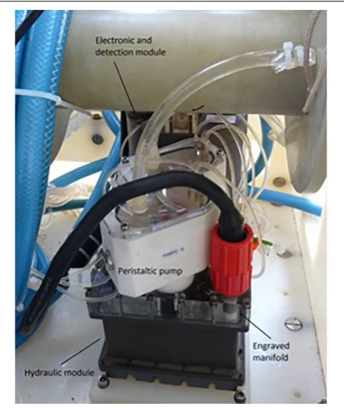
Laës-Huon et al., 2016), Mn (Klinkhammer, 1994; Okamura et al., 2001), and Cu (Holm et al., 2008) in coastal settings and in the vicinity of hydrothermal vents (Figure 2), there are currently no autonomous analytical techniques that can measure micronutrient metal species at the necessary detection limits for open ocean work.
FIGURE 2 |The CHEmical MINIaturized analyzer (CHEMINI) for iron determinations in the vicinity of hydrothermal vents implemented on the EMSO-Azores MoMAR observatory infrastructure at 1700 m depth, hydraulic module: 240∗150 mm, electronic module: 140∗264 mm (Laës-Huon et al.,
2016).
that are not responsive to temperature variations would be highly desirable.
Avoiding Contamination
Contamination is one of the major hurdles associated with trace metal analysis, and will require careful consideration in the design of autonomous analyzers housings (e.g., using metal free components such as Teflon or LDPE that are in contact with the sample), as well as the selection of non-contaminating platforms from which to deploy them. The extremely low natural concentrations of metals and their ubiquity in traditional sampling equipment (ships, frames, bottles) have led trace metal geochemists to develop extreme methodologies to avoid contamination during all phases of sampling and analysis. Specialized sampling systems for vertical profiling have been developed using polymer-based hydrowires and plastic-coated or titanium rosette frames fitted with sampling bottles that are lined with Teflon or constructed using high-purity plastics (de Baar et al., 2007; Measures et al., 2008; Cutter and Bruland, 2012). To avoid introduction of contaminants following recovery of the sampling package, subsampling is carried out in class 100 filtered air spaces and rigorously cleaned plastic containers are used for sample storage.In situmonitoring will obviously eliminate some of these issues, most notably during sample acquisition and
processing (filtration, acidification) and by removing the need to transfer and store the sample into a clean container prior to analysis. However, not all available deployment platforms will be suitable forin situ metal sensors. For example, deploying a sensor on a moored profiler will require the use of non-metallic components or the addition of vanes to orient the sensor intake upstream of the mooring line. Therefore, some existing ocean observing infrastructure (OOI) will need to be customized in order to accommodate new micronutrient sensors while other ocean observing assets may not be suitable at all.
Biofouling in oceanic environments can take place very quickly, particularly in surface waters during periods of high biological productivity, and can lead to data quality deterioration in less than a few weeks’ time (Delory and Pearlman, 2018). Processes to minimize biofouling effects are therefore necessary to ensure the long-term reliability ofin situmonitoring devices. Considering that the most effective biofouling prevention relies on the use of metals (e.g., Cu coatings), the development of metal-free biofouling coatings may be necessary to prevent contamination of metal sensors/analyzers, particularly in regions where sub-nanomolar metal concentrations are prevalent. The intricacies of trace metal analysis will thus potentially restrict the integration of newly developed metal sensors into existing ocean observing assets.
Metal Speciation
Metal micronutrients can exist in a variety of redox states, chemical species, and in a range of operationally defined physical forms. The majority of historical metal micronutrient observations consists of total dissolved concentrations, which are obtained following separation from the particulate phase using 0.2–0.45µm pore size filters and acidification to pH<2 using a strong acid. The total dissolved metal fraction includes colloids, organic and inorganic complexes, as well as free hydrated ions (<0.02µm), which may be the most bioavailable species to biota. The operationally defined total dissolved metal fraction has been adopted based on historic sample filter sizes. Acidification allows sample integrity to be preserved prior to analysis and for the comparison of data from one location to the other and among various analytical labs. It also allows organically complexed metals to be dissociated and thus make them accessible to the analytical methodology.
of in situ metal analyzers that do not require pre-treatment (filtration and acidification) may provide additional insights into the reactivity of metal micronutrients in their natural state, thereby providing measurements that are more representative of bioavailability than total dissolved concentrations. It would also simplify in situ chemical analyzer manifolds and increase their measurement frequency, by removing one analytical step characterized with slow kinetics (i.e., the liberation of metals from ligand complexes). However, if filtration is avoided, particulates and biofouling could limit long-term deployment by blocking channels of microfluidics systems. Further assessment is required to fully resolve this issue.
Long-Term Accuracy:
In Situ
Calibration
To maintain analytical accuracy over long (months) periods, micronutrient metal sensors will need to be calibrated autonomously and accuracy assessed through the use of external standards. In the case of sensors measuring total dissolved metal concentrations (i.e., filtered and acidified),in situcalibration can be performed using acidified onboard standard(s) run at regular intervals throughout the deployment period. The shelf life of acidified onboard standards for total metal determinations is not expected to be an issue, as illustrated by the long-term stability of the SAFe and GEOTRACES community standards, which have exhibited stable concentrations for a variety of metals over several years. Quality control will prove more challenging forin situspeciation determinations, since it will be more difficult to preserve the standard solution (e.g., Fe (II)) over extended deployment times.
Measurement Frequency, Data
Acquisition
End-users desire sensors that can be deployed for a minimum of 1 month and up to 12 months with confidence, have high measurement frequencies (hours to days;Table 1) and minimal servicing requirements. Ideally, these sensors would employ real-time satellite reporting of the metal micronutrient concentrations along with other ancillary biogeochemical parameters (e.g., T, S, Chl-a) to enable adaptive sampling. Increasing the measurement frequency, which depends on the environment, sampling mode and research questions, implies an increase in data storage capacities. For current metal micronutrient analysis onboard ships, post-cruise data processing (reagent blank, optical blank, electrochemical background subtraction) is carefully employed. Such high-quality corrections will need to be implemented for the next generation ofin situsensors and one of the next challenges would be to consider when and how to apply corrections from
in situ calibration or from in situ quality control. Globally accepted definitions of the speciation (physical, redox, chemical speciation) for metal micronutrients concentrations produced by sensors will also need to be considered before integrating them into databases and global models.
Fostering Widespread Use
The commercialization of plug-and-play micronutrient metal sensors with sub-nanomolar sensitivity is unlikely within the next
decade due to the relatively small market for such devices and the high costs associated with prototype development, validation, and manufacturing of the final product. For this reason, most micronutrient metal sensor development work will continue to be carried out at research institutions, where prototypes are engineered in house using specialized instrumentation with a high level of expertise for fabrication, operation, deployment, and data processing (e.g., Klinkhammer, 1994;Okamura et al., 2001; Holm et al., 2008; Laës-Huon et al., 2016). In addition, the development work required to convert early prototypes into robust, reliable, and validated instruments for month-long deployments in the open ocean spans across more than one typical 3–5 year funding cycle. It is also difficult to sustain using research funding schemes that often prioritize innovation over continued development and validation. Thus, emerging sensors rarely go beyond the prototype stage, which hinders extensive use by the wider community.
To foster widespread deployments, one possibility would be to promote the development of autonomous micronutrient analyzers assembled using commercially available or 3D printed components and operated using open-source electronics, microcontrollers, software, and instrument housings. This strategy, which proved popular with the Do It Yourself (DIY) environmental-sensor makers community, may facilitate the fabrication and operation of low cost wet-chemical micronutrient metal sensors and maximize replication and operation by a greater number of end users worldwide. Indeed, the current popularity of custom-made FIA manifolds for the analysis of trace micronutrients onboard ships may be attributed to the fact that these manifolds can be built using commercially available components that do not require a high degree of expertise for assembly and software control. Applying a DIY open-source strategy and readily available technology would greatly simplify the developmental pathway from laboratory to the ocean and would lower the overall costs of the development and production of wet chemical analyzers. This approach will likely attract more analytically inclined trace metal geochemists to participate in the development. Consequently, the community would greatly increase the number and capability of prototype analyzers for bioactive micronutrient metals that could be readily deployed and tested on short-term missions aboard autonomous surface vehicles or at coastal monitoring nodes. Such an increase in the number of sensors will ultimately lead to robust concentration reports of defined sets of intercalibrated metal species, determined with well-accepted sampling and analytical protocols.
TECHNOLOGIES WITH POTENTIAL
WITHIN A DECADE
Several analytical technologies have the potential to be deployed
TABLE 4 |Summary of attributes of potential techniques forin situmetal micronutrient determinations within the next decade.
Technique Advantages Disadvantages
Wet Chemical Analyzers
High resolution, accuracy, and precision Relatively fast response time
Can be calibratedin situ
Expensive
Many analyzers have high power requirements
Relatively bulky Biofouling
High maintenance costs
Longevity limited by reagent use and stability
Waste generation
Electrochemical methods
Inexpensive Easy to use
Large measurement range Speciation measurements Not influenced by turbidity
Lower resolution, accuracy, precision Subject to ionic interferences, organic matter
High instrument drift Biofouling
Difficult to calibratein situ Autonomous trace
metal clean samplers
Good starting point for remote locations with challenging environmental conditions (i.e., high latitudes) Multi-elemental determinations
Limited measurement frequency More prone to storage and contamination artifacts
Require expert shore-based analysis Biofouling
Passive preconcentration samplers
Inexpensive Easy to use No power source Preconcentration included Multi-elemental determinations
Lower resolution, accuracy, precision Require lab testing and intercalibration Integrative concentration measurement which is hard to calibrate
Require expert shore-based analysis
reagent stability and consumption, and (2) voltammetric sensors which are proven in high metal concentration environments (e.g., coastal systems, continental margins, and hydrothermal vent fields), and (3) passive preconcentration samplers, which have the potential to be mass deployed at low cost but will need to be recovered periodically for analysis, and thus will be most amenable to deployment in easily accessible coastal regions, where they could be incorporated in citizen monitoring programs.
Miniaturized Wet Chemical Analyzers
Lab-on-Chip
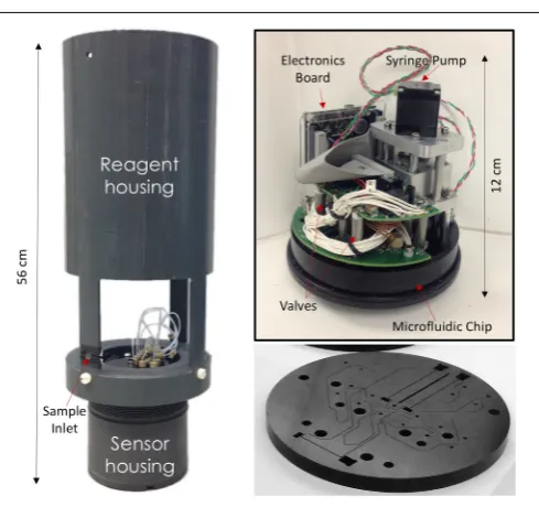
The miniaturization of existing reagent-based assays holds great promise for micronutrient sensing on moorings, cabled-arrays, and autonomous underwater vehicles (Statham et al., 2003, 2005; Gamo et al., 2007; Doi et al., 2008). Recent advances in microfabrication have led to the development of automated Lab-on-Chip microfluidic analyzers, which are compact, self-calibrating, fully automated, low cost, and operate standard absorbance methods with low power and reagent consumption (Figure 3). These instruments have been deployed for up to 2 months in estuarine and coastal settings, providing hourly macronutrient data (N, P) with an accuracy comparable to that of laboratory-based auto-analyzers (Beaton et al., 2012; Clinton-Bailey et al., 2017;Grand et al., 2017;Vincent et al., 2018). While fully automated Lab-on-Chip analyzers were recently developed for Fe (II) and Mn, their detection limits [2 nM, Fe(II),Geißler et al., 2017; 28 nM Mn, Milani et al., 2015] restrict their use to areas characterized by high concentrations, such as estuarine and coastal settings, oxygen minimum zones, and hydrothermal
FIGURE 3 |Lab-on-Chip phosphate analyzer. Left: fully assembled sensor with reagent housing. Top right: Analyzer prior to placement in watertight housing. Bottom-right: microfluidic chip showing micromilled fluidic manifold and absorbance flow cells prior to assembly. FromGrand et al. (2017).
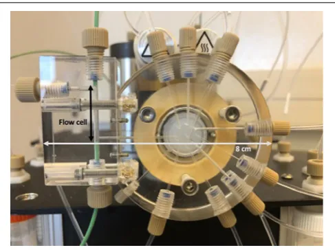
FIGURE 4 |Close-up of the lab-on-valve (LOV) module of a typical micro-Sequential Injection analyzer configured here for absorbance detection. The LOV can be configured for absorbance, fluorescence, or
chemiluminescence detection by repositioning the optical fibers (green tubing) around the flow cell and using appropriate detectors (e.g., miniature spectrophotometer, photomultiplier tube). The LOV ports are used to aspirate and mix microliter volumes of reagents and sample, which are then propelled to the flow cell for analyte quantification (rectangular block, left-hand side).
capabilities extended to fluorescence, chemiluminescence, and/or Cavity Ringdown Spectroscopy. These ongoing developments will enable Lab-on-Chip sensors to operate existing wet chemical assays for Mn, Fe, Zn, Cu, and Co within the next decade.
Micro-Sequential Injection Lab-on-Valve
Micro-Sequential Injection analyzers are another class of automated, miniaturized wet chemical analyzers with potential for in situ deployment (Figure 4). Presently best suited to laboratory and shipboard determinations (Oliveira et al., 2015;
Grand et al., 2016), these compact instruments share many of the features that have made FIA systems popular for shipboard metal micronutrient determinations. Indeed, Micro-Sequential Injection analyzers are made using commercially available components, are easily customizable, fully automated, and can operate absorbance, fluorescence, and chemiluminescence determinations coupled with analyte preconcentration to reach detection limits in the sub-nanomolar range. However, unlike FIA systems, they are characterized with low reagent consumption (100s of microliters per sample), are less prone to drift, and do not require much maintenance, which make micro-Sequential Injection analyzers better suited to long-term unattended operation relative to their FIA counterparts.
At present, the application of micro-Sequential Injection to micronutrient metal determinations at open ocean levels is limited to the shipboard analysis of total dissolved Zn and Fe, with reported detection limits of 50 pM for Zn (Grand et al., 2016) and 1 nM for Fe (II) (Oliveira et al., 2015). Micro-Sequential Injection is thus a proven analytical technology for sub-nanomolar metal micronutrient detection, but unlike Lab-on-Chip platforms, micro-Sequential analyzers have not yet been
engineered for in situ deployment. Further work is required to integrate all micro-Sequential Injection components (Lab-on-Valve, pump, detectors, electronics, and microcontroller) into compact, submersible housings, which will enable the deployment of micro-Sequential Injection analyzers at fixed locations (cabled observatories) and possibly for surface mapping applications onboard unmanned surface vehicles (e.g., wave gliders, Sail Drones, Autonomous Underwater Vehicles) in the decade following OceanObs’19.
Electrochemical Methods
One possibility forin situapplications of ASV is to use a solid working electrode instead of a mercury drop (Sundby et al., 2005; Luther et al., 2008). A new in situ copper microsensor using a vibrating gold microwire working electrode ( Gibbon-Walsh et al., 2012), an iridium wire counter electrode, and a solid state reference electrode made of AgCl coated with an immobilized electrolyte and protected with Nafion has recently been developed. This sensor is able to detect Cu at nanomolar concentrations in coastal waters (2.0±0.5 nM) and performs speciation measurements. The current version of the system has been deployed in situ for hydraulic, electronic, and pressure tests (2750 m) aboard the Nautilesubmarine (Cathalot et al., 2017). Although the detection limit is currently too high for open-ocean applications, it may be lowered by increasing the deposition step time, thereby offering another prospect for
in situ ASV determination of Cu at sub-nanomolar levels. Conditioning and electrochemical cleaning of the electrode remains, however, as for the classical in situ voltammetric systems, a considerable challenge.
For environmental systems such as hydrothermal vents, diffuse flow ridge flanks, seeps, and sediments that are metal sources with higher concentrations (micromolar) of Fe and Mn,in situ solid Au/Hg working electrodes, have been tested and calibrated to 5000 m and from 2 to 60◦
C (Luther et al., 2008; Cowen et al., 2012). These voltammetry systems have been operated using the Alvin submersible and the Jason II
ROV in dynamic flowing vent and diffuse flow waters. In such environments, autonomous systems have been deployed for up to 3 weeks. These systems are amenable to integration into Ocean Observing Initiative assets where power is not limited. Fast scan voltammetry techniques (∼2 s for complete data acquisition) were used without a stripping or preconcentration step due to the elevated metal concentrations in these environments. The method uses a 5 s conditioning or cleaning step so that multiple analytes can be detected simultaneously every 7–10 s to study the dynamics of the source waters in these environmental systems.
In Situ
Collection, Preservation, and
Preconcentration
Serial Automated Trace Metal Clean Samplers
developing the capability to collect and preserve trace metal clean seawater samples in situ would allow obtaining time-series in environments that are only accessible once a year and are characterized with challenging conditions for any newly developed sensor, such as in the Southern Ocean. Second, the application of proven, autonomous trace metal clean samplers would be extremely valuable for testing and intercalibration of future in situ analyzers and sensors. The technology for autonomous trace metal samplers is already available and mature enough to be deployed within the next decade. Examples include the MITESS sampler (Bell et al., 2002), the newly developed PRISM sampler (Mueller et al., 2018), ANEMONE-11 (Okamura et al., 2013), the commercially available McLane Labs Remote Access Sampler (RAS), and the Biogeochemical AUV sampler CLIO, which is currently under development at WHOI. Each of these different autonomous sampler types has different advantages and disadvantages for remote sampling of low level, trace metal clean open ocean seawater, and the type of application will determine which one(s) are suitable. Some further refinements may be necessary to optimize the sampler type for the project needs (e.g., endurance, type of deployment, ocean conditions).
Passive Preconcentration Samplers
A complementary approach to automated samplers and in situ
analysis of micronutrient metals is the development of passive sampling techniques. Passive sampling is based on the diffusion of the analyte across a porous membrane (hydrophobic or hydrophilic) into a receiver phase (solid or liquid), where the analyte is accumulated at a rate that is proportional to the external concentration. After a set deployment period (days, weeks, months), the sampler is retrieved, and back in the laboratory the analyte is extracted from the receiver phase and analyzed. Passive samplers thus provide a time-averaged weighted concentration of the species of interest, which, in contrast to discrete sampling, increases the likelihood of capturing intermittent sources and sinks. In addition, passive samplers have no moving parts, do not require a power source, are inexpensive, and could thus be mass deployed, particularly in coastal regions where they can be easily retrieved. Another notable feature of passive samplers is that they collect and pre-concentrate the analyte in one step, which is particularly beneficial for metal species present at sub-nanomolar levels in seawater.
There are several types of passive sampling devices that have been developed over the past 30 years. Among these, Diffusive Gradient Thin (DGT) Gels and, more recently, Polymeric Inclusion Membranes (PIMs) have been deployed in coastal and inland waters (Twiss and Moffett, 2002;Shiva et al., 2016;
Almeida et al., 2017), and appear to have the most potential for micronutrient metal determinations. DGTs were also used successfully (analyzing a suite of trace metals at sub-nanomolar level) on discrete samples from the Southern Ocean (Baeyens et al., 2011) and more recently aboard a SeaExplorer glider in the Mediterranean Sea (Baeyens et al., 2018). It should be noted that passive samplers collect samples over the time interval of the deployment. Thus, while they are more likely to collect
transient signals over the time interval of the deployment, they will also average all transient signals over the time interval of the deployment. Prior to widespread use, these techniques will require further laboratory testing and validation to determine which metals species are being measured (free ions and small and possibly weaker metal–ligand complexes), and to quantify metal concentrations, given poorly constrained diffusion rates.
A ROADMAP TOWARD AUTONOMOUS
MICRONUTRIENT OBSERVING
SYSTEMS
There are several regions (e.g., high latitudes) and specific episodic processes (e.g., seasonal transitions) that would greatly benefit from high-resolutionin situmetal measurements in order to characterize and quantify sources and sinks of trace metals in the global ocean. Sensor development would also address an urgent need to improve predictions, in a rapidly changing ocean, of the plankton response (phytoplankton, bacteria, and archaea) to variations in micronutrient concentrations, following episodic events and/or at seasonal transitions.
Of the bioactive metal micronutrients (Fe, Zn, Co, Mn, Co, Ni, and Cd), Fe has received the most attention considering that it limits primary productivity in large parts of the world’s ocean, and imparts a significant influence on phytoplankton species composition. As such, Fe should probably be the prime target for sensor development and field implementation in the next decade, not only to improve the quantification of fluxes but also to better constrain the parameterizations of regional and global numerical models (Tagliabue et al., 2016). In addition, the technology and lessons learned from the development of an open ocean Fe sensor could facilitate the development of sensors for other important metal micronutrients, particularly for reagent-based analyzers which will operate using similar fluidic architectures and detection schemes. However, subsequently, high-frequency observations would be desirable for the full suite of essential trace elements, such as zinc (Southern Ocean:Vance et al., 2017; subarctic North Pacific:Kim et al., 2017).
Testing and Intercalibration
Development of metal sensors for remote deployment requires analyzers/sensors that are well tested in terms of electronic performance, endurance, and analytical performance under all operating conditions (i.e., freezing conditions and remoteness). Thus, before implementing in situ chemical analyzers, electrochemical sensors, and passive samplers on various types of platforms, the systems must be rigorously tested and validated under controlled laboratory conditions. Such long-term unattended laboratory tests should be standardized and include (1) temperature and pressure effects on analytical sensitivity, drift, and reagent shelf life (for methods sensitive to such changes, e.g., Okamura et al., 2001; Weeks and Bruland, 2002); (2) aging of the sensor (sunlight, seawater spray, vibrations); (3) the potential for biofouling and ways to mitigate it without metal-based biocides; and (4) a thorough intercalibration of the analyzer/sensor data quality (including speciation) with that of established techniques with input and guidance from the GEOTRACES community of analysts. These tests, which should at least be performed over a month-long period, will provide a first estimate of required operational settings in terms of robustness, reliability over time (figure of merits, drift), and lifetime without maintenance and power consumption, each of which will depend on the environmental conditions of the deployment and the analytical measurement frequency required for a given application. Such tests are theoretically feasible using existing monitoring platforms, pressure chambers, and test pools. However, as mentioned above, these tests are difficult to sustain beyond the typical 3–5 year time scale of a typical method development research grant and require resources that are not available to all developers (i.e., pressure chambers and test pools). Yet, they are critical to ensure end-users’ acceptance and foster widespread usage by the community.
Surface Mapping Along Dry and Wet
Atmospheric Deposition Gradients
Areas where dust deposition is important would be well served by the addition of high-frequency measurements. Dust deposition is an important source of trace metals to the open ocean, especially for Fe, whose availability influences productivity at high latitudes and nitrogen fixation rates in oligotrophic subtropical gyres (Tagliabue et al., 2017and references therein). Regions of known elevated dust deposition (e.g., the subtropical North Atlantic; Sedwick et al., 2005; Buck et al., 2010) would be expected to exhibit large dissolved metal gradients at concentrations significantly above other open ocean locations, thereby facilitating the establishment of new sensor systems. High-resolution autonomous surface mapping in these regions could improve understanding of the variables affecting metal dissolution including rainfall, dry deposition, and the sea surface microlayer, all of which are currently not well understood given the paucity of data at appropriate spatial and temporal resolution (Baker et al., 2016). Such measurements could also allow examination of the residence time of Fe in the surface ocean and the impact of deposition events on biological activity.
Although not a bioactive trace metal micronutrient, aluminium (Al) is considered a good proxy for dust deposition and thus the input of Fe to the surface ocean (Measures and Vink, 2000; Grand et al., 2015a; Anderson et al., 2016). The residence time of Al is considerably longer than that of Fe, but much shorter than that of Mn, suggesting that it reflects Fe inputs on a daily-to-annual time scale. Current benchtop analytical techniques (e.g., Resing and Measures, 1994) are sensitive enough to analyze Al in areas of intense dust deposition without a preconcentration step, making the development of an Al sensor for these areas an interesting proposition. Such a sensor would certainly complement any new Fe sensor and would provide a data set to evaluate changes in Fe inputs. This vision could be achieved within a decade, for example, by deploying Fe and Al analyzers on autonomous surface sampling vehicles, such as Wave Gliders and Sail Drones, for month-long missions. Sail Drones are perhaps most amenable to hosting prototype
in situwet chemical analyzers due to their power availability, size, and availability of dry instrument space above the water line (Voosen, 2018).
Time Series
Metal micronutrient time series are rare. They are mainly focused on Fe, of limited temporal resolution and difficult to maintain over the time period needed to decipher seasonal variations, episodic events, and their impact on marine ecosystem dynamics (Boyle et al., 2005; Sedwick et al., 2005; Nishioka et al., 2011;
Fitzsimmons et al., 2015; Barrett et al., 2015). Developing the capacity to instrument coastal and open ocean time-series sites, which are well characterized and visited on a regular basis for sampling and servicing (e.g., BATS, HOT, CalCOFI), would be a very desirable outcome in the decade following OceanObs’19. Ocean observing sites that are already instrumented with a mooring would be a good place to start (e.g., Ocean Station Papa, OOI Endurance Array) considering that power-hungry analyzers with relatively large payloads could be deployed and serviced at regular intervals during their development stages.
transport of Fe could be explored further using a series of analyzers deployed in the wake of a vent system (Waeles et al., 2017). Metal fluxes from reducing sediments and the metal dynamics in oxygen minimum zones characterized by elevated metal concentrations could also be explored. For example, trace metal sensors could be integrated with existing ocean observing assets, such as the long-term time sampling program in Saanich Inlet (BC, Canada), a low-oxygen fjord, with monthly monitoring measurements, and a VENUS cabled observatory (Ocean Networks Canada). The implementation of such systems should be easily accomplished as it has already been performed on one of the deepest parts of the Ocean Networks Canada (Grotto Hydrothermal Vent, Endeavour Field, 2186 m) from 2011 and 2013 to collect iron concentrations (CHEMINIin situanalyzer) and to link them to the chemosynthetic environment and its related fauna (Cuvelier et al., 2014, 2017).
CONCLUSION AND
RECOMMENDATIONS
Trace metal biogeochemistry is integral to our understanding of marine biogeochemical cycling and ocean productivity. The next decade offers the opportunity to capitalize on the findings of the GEOTRACES program, and the growing Ocean Observatories Initiative (assets, autonomous vehicles) to investigate processes and regions at the spatial and temporal resolution necessary to constrain fluxes, residence times, and biological and chemical responses to varying metal inputs and distributions in a changing ocean. Capitalizing on this opportunity, however, requires the development of sensors capable of measuring trace metal micronutrients at levels found in the open ocean. In the next decade, we can make progress with the development of techniques with increased sensitivity and sensor support infrastructure. In addition, we can deploy existing flow techniques, electrochemical methods, and passive samplers on dry platforms including moorings, Sail Drones, autonomous underwater vehicles, ocean observing assets, and ships of opportunity.
To meet this opportunity, however, significant resources must be invested to accomplish goals on several fronts. The first is the improvement in the analytical sensitivity of existing sensors, chemical analyzers, and their underlying chemistries. Novel chemical assays must be developed for those underlying chemistries that employ stable reagents and that are insensitive to temperature variations. Secondly, we must reduce sensor size and power requirements. In addition to deploying existing techniques, it is essential to develop an open-source “DIY” infrastructure to allow ease of sensor development and a mechanism by which scientists can rapidly adapt commercially available technology to in situ applications. Finally, to meet this opportunity, sensor technologies will need to demonstrate the endurance and comparability of in situ sensor data with established techniques in controlled lab conditions. Each of these areas will best be served through interdisciplinary collaborations/joint proposals with government, industry, or academic partners. The creation of an international working group of trace metal
sensor developers facilitating regular meetings and workshops and involving the engineering, oceanographic, and analytical chemistry communities could accelerate the delivery of new technology that can be applied to in situmetal determinations in the decade following OceanObs’19.
It should be noted that no sensor is likely to be appropriate for every application. Thus, at this stage, no particular technology should be preferred over another. For example, while wet chemical techniques may ultimately provide the best sensitivity for open-ocean applications, such sensors will be limited by their longevity in the field and may not be applicable to autonomous profilers that are not recovered, due to power usage and analytical throughputs incompatible with profiling rates (i.e., Argo floats). In this regard, recent developments in analytical chemistry (novel ligands, fluorophores, ionophores, biosensors, miniaturized methods) should be regularly evaluated for their oceanographic potential.
The development of the discussed technologies are of great benefit to society as they will allow an ever greater understanding of ocean and climate feedbacks associated with the input and cycling of trace elements in the ocean. Ocean sampling programs such as GEOTRACES are vastly improving the understanding of dynamics of trace elements and in many instances allow understanding and identification of processes for the first time, in addition to prompting reconsideration of historical paradigms (e.g.,Resing et al., 2015). This is largely due to the collaborative nature of these projects that make concurrent observations of multiple trace elements and relevant biogeochemical data over large sections of the world’s ocean. These large-scale discrete measurements also provide much desired information on trace metal sources and sinks. However, these ocean sections do not provide a full measure of spatial variability and no measure of temporal variability that we expectin situsensors to provide.
Understanding trace metal dynamics has a wide range of applications, including improving our understanding of oceanic water mass circulation, surveying, and understanding toxic metal plumes and algae. Spatial and temporal observations by micronutrient metal sensors will facilitate significant improvements of numerical models that predict carbon uptake and export to the deep ocean, and thus will provide a better understanding of the role of the ocean in regulating climate. Trace metals are also of societal concern, as they may reflect pollution and in some cases their presence may be detrimental to the base of the food web. Such pollution can occur in coastal regions, as well as the open ocean through dust deposition. By understanding the variability of trace metals we can better understand their impacts on phytoplankton species composition, including the presence of harmful algae blooms. Ultimately, ecosystem management will be better informed by the addition of high-quality data that is rapidly produced and readily available on meaningful time scales.
AUTHOR CONTRIBUTIONS
by MG, to the writing and editing of previous versions of this manuscript, and gave final approval for publication. AT compiled the global database of dissolved measurements in the ocean that are used to createFigure 1.
FUNDING
GL acknowledges support from the Chemical Oceanography Program of NSF (OCE-1558738). JR was supported by
the Joint Institute for the Study of the Atmosphere and Ocean (JISAO) under NOAA Cooperative Agreement NA15OAR432 0063.
ACKNOWLEDGMENTS
We thank Ed Urban and Maite Maldonado for launching this contribution to OceanObs’19 and for editing an earlier version of this manuscript. This is JISAO publication #2018-0177 and PMEL #4887.
REFERENCES
Achterberg, E. P., and Braungardt, C. (1999). Stripping voltammetry for the determination of trace metal speciation and in-situ measurements of trace metal distributions in marine waters.Anal. Chim. Acta400, 381–397. doi: 10.1016/ S0003-2670(99)00619-4
Achterberg, E. P., and van den Berg, C. M. G. (1994). In-line ultraviolet-digestion of natural water samples for trace metal determination using an automated voltammetric system. Anal. Chim. Acta 291, 213–232. doi: 10.1016/0003-2670(94)80017-0
Achterberg, E. P., and van den Berg, C. M. G. (1996). Automated monitoring of Ni, Cu and Zn in the Irish Sea.Mar. Pollut. Bull.32, 471–479. doi: 10.1016/0025-326X(96)84963-0
Almeida, M. I. G. S., Cattrall, R. W., and Kolev, S. D. (2017). Polymer inclusion membranes (PIMs) in chemical analysis – A review.Anal. Chim. Acta987, 1–14. doi: 10.1016/J.ACA.2017.07.032
Anderson, R. F., Cheng, H., Edwards, R. L., Fleisher, M. Q., Hayes, C. T., Huang, K.-F., et al. (2016). How well can we quantify dust deposition to the ocean?
Philos. Trans. A Math. Phys. Eng. Sci.374:20150285. doi: 10.1098/rsta.2015. 0285
Baeyens, W., Bowie, A. R., Buesseler, K., Elskens, M., Gao, Y., Lamborg, C., et al. (2011). Size-fractionated labile trace elements in the Northwest Pacific and Southern Oceans.Mar. Chem.126, 108–113. doi: 10.1016/j.marchem.2011.04. 004
Baeyens, W., Gao, Y., Davison, W., Galceran, J., Leermakers, M., Puy, J., et al. (2018). In situ measurements of micronutrient dynamics in open seawater show that complex dissociation rates may limit diatom growth.Sci. Rep.8:16125. doi: 10.1038/s41598-018-34465-w
Baker, A. R., Landing, W. M., Bucciarelli, E., Cheize, M., Fietz, S., Hayes, C. T., et al. (2016). Trace element and isotope deposition across the air–sea interface: progress and research needs.Philos. Trans. A Math. Phys. Eng. Sci.
374:20160190. doi: 10.1098/rsta.2016.0190
Barrett, P. M., Resing, J. A., Buck, N. J., Landing, W. M., Morton, P. L., and Shelley, R. U. (2015). Changes in the distribution of Al and Fe in the eastern North Atlantic Ocean 2003-2013: implications for trends in dust deposition.Mar. Chem.177, 57–68. doi: 10.1016/j.marchem.2015.02.009
Beaton, A. D., Cardwell, C. L., Thomas, R. S., Sieben, V. J., Legiret, F.-E., Waugh, E. M., et al. (2012). Lab-on-chip measurement of nitrate and nitrite for in situ analysis of natural waters.Environ. Sci. Technol.46, 9548–9556. doi: 10.1021/ es300419u
Bell, J., Betts, J., and Boyle, E. A. (2002). MITESS: a moored in situ trace element serial sampler for deep-sea moorings.Deep Sea Res. I 49, 2103–2118. doi: 10.1016/S0967-0637(02)00126-7
Biller, D. V., and Bruland, K. W. (2012). Analysis of Mn, Fe, Co, Ni, Cu, Zn, Cd, and Pb in seawater using the Nobias-chelate PA1 resin and magnetic sector inductively coupled plasma mass spectrometry (ICP-MS).Mar. Chem.
13, 12–20. doi: 10.1016/j.marchem.2011.12.001
Bowie, A. R., Achterberg, E. P., Mantoura, R. F. C., and Worsfold, P. J. (1998). Determination of sub-nanomolar levels of iron in seawater using flow injection with chemiluminescence detection.Anal. Chim. Acta361, 189–200. doi: 10. 1016/S0003-2670(98)00015-4
Bowie, A. R., Achterberg, E. P., Sedwick, P. N., and and. Worsfold, P. J. (2002). Real-time monitoring of picomolar concentrations of Iron(II) in marine waters
using automated flow injection-chemiluminescence instrumentation.Environ. Sci. Tech.36, 4600–4607. doi: 10.1021/ES020045V
Boyle, E. A., Bergquist, B. A., Kayser, R. A. R., and Mahowald, N. (2005). Iron, manganese, and lead at Hawaii Ocean time-series station ALOHA: temporal variability and an intermediate water hydrothermal plume.Geochim. Cosmochim. Acta69, 933–952. doi: 10.1016/j.gca.2004.07.034
Braungardt C. B., Achterberg, E. P., Axelsson, B., Buffle, J., Graziottin, F., Howell, K. A., et al. (2009). Analysis of dissolved metal fractions in coastal waters: an inter-comparison of five voltammetric in situ profiling (VIP) systems.Mar. Chem.114, 47–55. doi: 10.1016/j.marchem.2009.03.006
Bruland, K. W., Middag, R., and Lohan, M. C. (2014). Controls of trace metals in seawater.Treatise Geochem.6, 23–47. doi: 10.1016/B978-0-08-095975-7. 00602-1
Buck, C. S., Landing, W. M., Resing, J. A., and Measures, C. I. (2010). The solubility and deposition of aerosol Fe and other trace elements in the North Atlantic Ocean: observations from the A16N CLIVAR/CO2 repeat hydrography section.
Mar. Chem.120, 57–70. doi: 10.1016/j.marchem.2008.08.003
Cathalot, C., Heller, M. I., Dulaquais, G., Waeles, M., Coail, J. -Y., Kerboul, A., et al. (2017). ELVIDOR- vibrating gold micro-wire electrode:In situhigh resolution measurements of Copper in marine environments, Goldschmidt Abstracts, 584. Chapin, T. P., Jannasch, H. W., and Johnson, K. S. (2002). In situ osmotic analyzer for the year-long continuous determination of Fe in hydrothermal systems. Anal. Chim. Acta 463, 265–274. doi: 10.1016/S0003-2670(02) 00423-3
Chapman, C. S., Cooke, R. D., Salaün, P., and van den Berg, C. M. G. (2012). Apparatus for in situ monitoring of copper in coastal waters.J. Environ. Monit.
14, 2793–2802. doi: 10.1039/c2em30460k
Chin, C. S., Coale, K. H., Elrod, V. A., Johnson, K. S., Massoth, G. J., and Baker, E. T. (1994). In situ observations of dissolved iron and manganese in hydrothermal vent plumes, Juan de Fuca Ridge.J. Geophys. Res. Solid Earth99, 4969–4984. doi: 10.1029/93JB02036
Chin, C. S., Johnson, K. S., and Coale, K. H. (1992). Spectrophotometric determination of dissolved manganese in natural waters with 1-(2-pyridylazo)-2-naphthol: application to analysis in situ in hydrothermal plumes.Mar. Chem.
37, 65–82. doi: 10.1016/0304-4203(92)90057-H
Clinton-Bailey, G., Grand, M., Beaton, A., Nightingale, A., Owsianka, D., Slavik, G., et al. (2017). A lab-on-chip analyzer for in situ measurement of soluble reactive phosphate: improved phosphate blue assay and application to fluvial monitoring.Environ. Sci. Technol. 51, 9989–9995. doi: 10.1021/acs.est.7b01581 Coale, K. H., Johnson, K. S., Fitzwater, S. E., Gordon, R. M., Tanner, S., Chavez, F. P., et al. (1996). A massive phytoplankton bloom induced by an ecosystem-scale iron fertilization experiment in the equatorial Pacific Ocean.Nature383, 495–501. doi: 10.1038/383495a0
Cowen, J. P., Copson, D. A., Jolly, J., Hsieh, C.-C., Lin, H.-T., Glazer, B. T., and Wheat, C. G. (2012). Advanced instrument system for real-time and time-series microbial geochemical sampling of the deep (basaltic) crustal biosphere.
Deep-Sea Res. I61, 43–56. doi: 10.1016/j.dsr.2011.11.004
Croot, P. L., Moffett, J. W., and Luther, G. W. III (1999). Polarographic determination of half-wave potentials for copper-organic complexes in seawater.Mar. Chem.67, 219–232. doi: 10.1016/S0304-4203(99)00054-7 Cutter, G. A., and Bruland, K. W. (2012). Rapid and non contaminating sampling
system for trace elements in global ocean surveys.Limnol. Oceanogr. Methods