MoL 2005 02: The Value of Agreement: a new Boosting Algorithm

Boaz Leskes

The Value of Agreement

a new boosting algorithm

Master Thesis

Section Computational Science

and

Institute for Logic, Language & Computation

University of Amsterdam

Abstract

Contents

1 Introduction 1

1.1 The Co-training model . . . 2

1.2 Boosting . . . 4

2 The Value of Agreement 7 2.1 Preliminaries . . . 7

2.2 Formal Settings . . . 9

2.3 Reduction of labeled examples . . . 13

3 The Algorithm 15 4 Proof of convergence 17 5 Experiments 27 5.1 A toy problem . . . 27

5.1.1 Results . . . 28

5.2 Classifying web pages . . . 30

5.2.1 Naive Bayes for Text Classification . . . 30

5.2.2 Agreeing with the Village Fool... . . 31

5.2.3 Using a better learner . . . 33

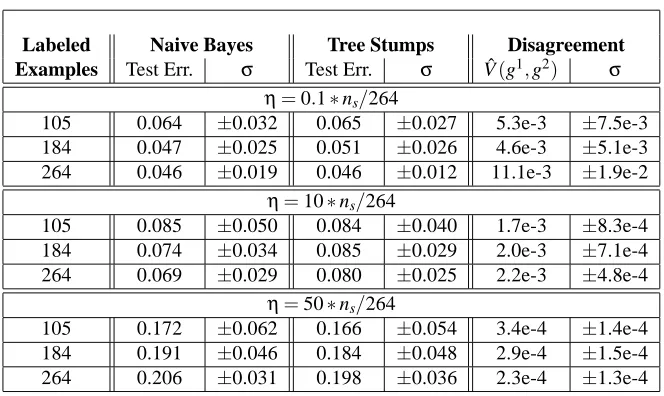
5.3 Agreeing is important, but how much? . . . 37

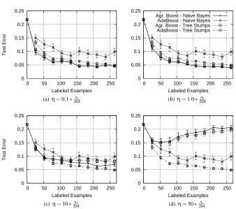
5.3.1 Setting theηparameter . . . 37

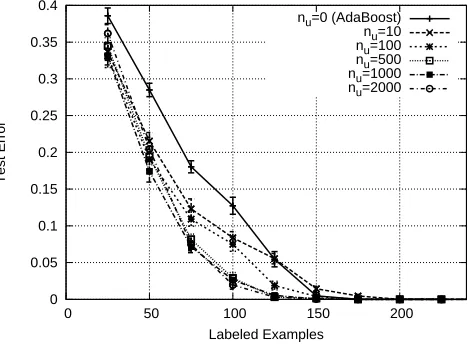
5.3.2 The effects of the number of unlabeled examples. . . 39

Chapter 1

Introduction

Imagine a young pupil being taught for the first time to read a foreign language. The teacher might begin the first lesson by writing the entire alphabet of the language on the board announcing that today they are going to learn the first letter, say ‘ℵ.’ After a rather cumbersome hour of staring at letters, the pupil is surprised by the teacher’s last announcement: the following lesson will begin with a short quiz covering today’s material. The quiz will take the following form: each pupil will receive a sheet of paper written in that foreign language and will have to mark all occurrences of the letter ‘ℵ.’ Furthermore, imagine that the teacher of this young pupil is a particularly bad one. She does not give the pupil any guidance nor explanation with respect to how an ‘ℵ’ should be recognized out of the whole alphabet. Rather the teacher spends the whole lesson showing the students transparencies of different letters, saying for each one whether it is a nice example of the lesson’s subject (‘ℵ’) or that it is a letter they will study at a later time.

The problem faced by this poor pupil can be modeled by one of the simplest but popular models in machine learning called supervised learning. This model represents a scenario where a ‘learner’ is required to solve a classification problem. The model assumes the existence of a set of possible examples

X

which are divided in some way into a set of classes

Y

(often called labels). In the pupil’s case, the example space can be the set of all possible images of letters in the alphabet (one letter per image) and the classes are ‘ℵ’ and non-‘ℵ.’ The pupil then comes up with a mapping f :

X

_→

Y

, saying for each letter in the quiz whether it is an ‘ℵ’ or not. In order to evaluate the quality of the pupil’s mapping it is assumed that there exists a distribution P over

X

_×

Y

which represents the ‘chance’ to see a specific example and it’s label1in real life. The quality of the pupil’s mapping, or classifier, is then measured by the probability of it making a mistake. In other words, the lower the probability of the classifier making a mistake, the better the classifier.

In class, the only interaction between teacher and pupil is achieved by showing the pupil a set of examples along with their correct label. This form of interaction is modeled by assuming that the learner is given a finite sample of labeled examples S, drawn at random and independently from P. Since this is the only information the pupil receives, she must use this sample to generate the resulting classifier.

More formally, the learning model is defined as follows: it is assumed that the learning algorithm is given only a finite sequence of training examples. The training

1_{Note that this setting allows an example to belong to different classes, or have several labels. This is}

examples are given in the form of a set of ordered pairs, S=(xj,yj) ns_j=1, where each instance xj belongs to some instance space

X

and is accompanied by a single label out of a label space2

Y

_⊆[−1,+1]. Furthermore, it is assumed that the training set S was generated by repeatedly and independently sampling some arbitrary probability distribution P over

X

_×

Y

. The task of a learning algorithm is then to use the training set to construct a classifier, or a hypothesis that best predicts the labels given to ex-amples from

X

by P. Typically the learning algorithm can only choose a hypothesis from a limited set of possible hypotheses, which is referred to as the hypothesis space H_⊆

Y

X.

Though the above learning scenario is somewhat contrived, many real life applica-tions fall nicely within this model. Problems like OCR, web pages classification (as done in Internet directories) and detection of spam e-mail are only a few of many prob-lems that fit into this scheme. Note that the assumption regarding the poor didactic skills of the teacher is made to serve a very practical reason: how does one explain to an e-mail program how to detect a spam e-mail? If this was easy, it would have been much simpler to write a program to identify spam rather then running a learning algorithm. Devising concrete rules that precisely discern spam from non-spam is much harder (to humans) than the pure proclamation “This is spam.” In other words, the al-gorithm is used to transfer our somehow vague notion of “This is spam” to a concrete rule that can be efficiently executed by a computer. Therefore, an algorithm that is able to ‘learn’ concrete classification rules from a labeled sample alone demands less from the ‘teacher’—the user of the learning algorithm.

In all the examples above and in many others, it is relatively hard to obtain a large sample of labeled examples. The sample has to be carefully analyzed and labeled by humans—a costly and time consuming task. However in many situations it is fairly easy to obtain unlabeled examples: examples from the example space

X

without the class that they belong to. This process can be easily mechanized and preformed by a machine, much faster then any human-plausible rate. This difference between labeled and unlabeled examples has encouraged researchers in the recent years to study the benefits that unlabeled examples may have in various learning scenarios. For example, will it help the young pupil if she will be given a booklet written in that foreign lan-guage to take home? Can this booklet and the abundant unlabeled-examples within be used to improve the pupil’s results in the coming exam?

1.1

The Co-training model

At first glance it might seem that nothing is to be gained from unlabeled examples. After all, unlabeled examples lack the most important piece of information—the class to which they belong. However, this is not necessarily the case. In some theoretical settings, it is beneficial to gain knowledge over the examples’ marginal distribution P(x)(for example in [7]). In these cases, having extra examples, with or without their label, provides this extra information. On the other hand, there exist situations (for example in [10]) where knowing P(x)is not helpful and unlabeled examples do not help at all. The main goal of this sort of research is to determine the amount of information that can be extracted from unlabeled examples. However, unlabeled examples have also been used by algorithms in a more practical way: as a sort of a communication

2_{For technical reasons, the label space is restricted to[}

The Value of Agreement A New Boosting Algorithm

platform between two different learning algorithms. One such usage is the so called Co-Training model or strategy.

A typical example of Co-Training can be found in [5], a paper often cited with respect to unlabeled examples. In their paper, Blum and Mitchel provide both an algo-rithm and a theoretical framework where unlabeled examples are used to communicate an ‘opinion’ about an unlabeled example from one algorithm to another. As a case study, the algorithm is then applied to a web-page classification problem involving identifying courses’ homepages out of a collection of web-pages.

In their work, Blum and Mitchel assume that the example space can be split into two ‘views’

X

1_and

_X

2_i.e.,

_X

₌

_X

1_×

_X

2_{. For example, in the web-page classification}

problem, a web-page can be represented as the words appearing on the web-page itself (view 1) but also as words appearing on links pointing to it. Further they assume that examples are labeled by two target functions f1,f2, one for each view. In order to comply with the fact that each example belongs to a single class, they further assume that P x1_×x2_{: f}1 _x1_6=f2 _x2 _{=0. Lastly, they assume that there exist two}

learning algorithms L1 and L2 such that L1 can learn using the first view alone and L2 can learn using the second view and in the presence of noise. Furthermore, they suppose that both views are sufficient for learning the problem.

The main theoretical result in their paper is the following: under some assumptions, a classifier that uses the first view and that is slightly better than random guessing is equivalent to a noisy source when looked upon from the point of view of L2. Further-more, the noise rate of the source is strictly smaller than 1₂ and therefore it contains some information on the original labels. If L1is trained on the labeled examples to achieve such a classifier, it can then be used to label unlabeled examples and supply a noisy source for L2to learn from. Since L2can learn in the presence of noise, it can then use the abundant newly labeled examples to produce a good classifier.

This ability to transform a deterministic process to random noise entails a very severe assumption: for every fixed example xˆ1,xˆ2_∈

X

of non-zero probability it must hold that:

P X1=xˆ1_|X2=xˆ2 = P X1=xˆ1_|f2 X2= f2 xˆ2 (1.1) P X2=xˆ2_|X1=xˆ1 = P X2=xˆ2_|f1 X1= f1 xˆ1.

In other words, that X1and X2are conditionally independent given the label. As the authors themselves state, only four hypotheses comply with this assumption (assuming that P allows for it).

Algorithm 1 The Co-Training algorithm, as presented in [5]

Inputs:

• A set of labeled training examples (S)

• A set of unlabeled examples(U)

1. Create a pool U0 of examples by choosing nuunlabeled examples, at random, from U .

2. Loop for k iterations:

(a) Use S and L1to train a classifier h1that considers only the x1portion of the examples.

(b) Use S and L2to train a classifier h2that considers only the x2portion of the examples.

(c) Allow h1to label p positive and n negative examples from U0.

(d) Allow h2_{to label p positive and n negative examples from U}0_.

(e) Add these self-labeled examples to S.

(f) Randomly choose 2p+2n examples from U to replenish U0.

are encouraged to agree on a set of examples whose labels were not given to them in advance. Before starting the algorithm, there is no guarantee as to what label an unla-beled example will receive but only to the fact that the end classifiers are highly likely to agree on that label. This type of agreement is a side effect of many other variants of the co-training model [15, 14].

This intuition that agreement is useful and can assist in the task of learning is elabo-rated and made more precise in this paper. A theoretical framework is presented where agreement between different learners has a clear advantage3_{. Furthermore, these ideas}

are carried over to the field of boosting, where the theoretical settings are especially ap-plicable. This is achieved in the form of a new algorithm that builds upon this theory. A similar attempt can be found in [17] where a boosting algorithm is presented, based on the above intuition. However, no proof is provided that the algorithm does result in agreeing classifiers nor for the advantage of such an agreement. A proof for the latter (in a more general settings) was provided by Dasgupta et al. in [18]. Nevertheless, for the proof to hold one still has to use the strong assumption of view-independence (Equation 1.1). Another example for the use of unlabeled examples in boosting can be found in [23].

Before delving into the theoretical benefits of agreement, we present a short intro-duction to boosting.

1.2

Boosting

The basic idea behind boosting is to iteratively combine relatively simple hypotheses to create a more complex classifier—a classifier that is superior to all underlying

The Value of Agreement A New Boosting Algorithm

Algorithm 2 AdaBoost [19]

Input: A sample S={(xi,yi)}ns_i=1and an underlying learning algorithm L. 1. Initialize: d_i(1)=1/nsfor all i=1, . . . ,ns.

2. Do for t=1, . . . ,T :

(a) Use L to obtain a hypothesis ht:

X

→ {−1,+1}trained on S, re-weighted according to d(t).

(b) Calculate the weighted training errorεt of ht:

εt= ns

∑

i=1

d_i(t)I(yi6=ht(xi))where I(yi6=ht(xi)) =

1 if yi6=ht(xi)

0 otherwise

(c) Setαt=1₂log1−_εtεt.

(d) Update weights: d_i(t+1)=d_i(t)exp(−αtyiht(xi))/Zt, where Zt is a normal-ization constant such that ns∑

i=1

d_i(t+1)=1.

3. Output sign

_T

∑

t=1αt

ht

as resulting classifier.

ses. While coming up with a classifier (and an algorithm to construct it) that can ade-quately solve a supervised learning problem is hard, devising a ‘rule of thumb’ which is just slightly better than random guessing is fairly easy in many problems. Take, for example, the web-page classification problem from before. One can use the existence of the word ‘course’ in a web-page as a relatively good indication that this is a course home page. While this criterion is far from perfect (for example, a university schedule is also highly likely to contain the word ‘course’) it is still much better than random guessing. Other such words may include ‘homework’,‘class’,‘lesson’,‘assignment’ etc. In the last decade boosting has grown in popularity and has received consider-able attention. One of the first practical boosting algorithms was AdaBoost (Adaptive

Boosting, see Algorithm 2), introduced by Freund and Schapire in [19]. Since then, it

was thoroughly researched and many variants of it were derived. Since AdaBoost is such a typical and simple boosting algorithm, it will be used here as a representative example.

The main idea behind AdaBoost (and many other boosting algorithms) is to assign to each of the training examples a weight. An underlying learning algorithm is then used to generate a (weak) hypothesis based on this artificially weighted training set. This means that the algorithm receives the original training set S along with the weights of examples in it. The learning algorithm is expected to treat this weighing as if it is the true distribution of examples in S.

giving more weight to hypotheses that had a lower classification error.

Freund and Schapire provide a bound for the training error made by the ensemble classifier built by AdaBoost:

1 ns

ns

∑

i=1

I(yi6=sign(f(xi)))≤2T T

∏

t=1

p

εt(1−εt).

If it is further assumed that weak learning algorithm always returns a hypothesis whose error is at least a constant away from random guessing (i.e.,εt ≤1₂−γ), this bound turns into:

1 ns

ns

∑

i=1

I(yi6=sign(f(xi)))≤exp −2Tγ2

.

Therefore, under the above assumption, the training error decays exponentially fast. This quick convergence has also been observed in practice and is one of the most important traits of AdaBoost.

Further experiments have revealed that this analysis is not enough to explain the behaviour of AdaBoost. Typically, the reduction of training error to zero was combined with a generalization4bound connecting the training error to the global true error of the classifier (for an example, see Theorem 12 in Chapter 2.3). This means that once a classifier has reached zero training error the bounds have reached their full power in predicting the quality of it. However, in practice, the test-error of the classifiers produced by AdaBoost continue to improve long after the training error has reached zero.

Beginning with [20], a whole new set of generalization bounds was introduced that can explain this behavior. Two of these bounds will be presented in the following chapters as an example. Describing the rest of the generalization bounds and the huge amount of research into and improvements of AdaBoost is far beyond the scope of this work. For further information and an excellent introduction, the reader is referred to [1].

4_{The term generalization refers to the ability of a classifier to perform well in general and not only on}

Chapter 2

The Value of Agreement

In this chapter, a theoretical foundation and justification of the advantage in combing several different learning algorithms will be presented.

A typical approach in the supervised learning model is to design an algorithm that chooses a hypothesis that in some way best fits the training sample. It will be shown that an advantage can be gained by taking several such learning algorithms and de-manding that they not only best learn the training set but also ‘agree’ with each other by outputting identical hypotheses1.

The discussion below involves several learning algorithms and their accompanying hypothesis spaces. To avoid confusion, any enumeration or index that relates to dif-ferent learners or hypotheses is enumerated using superscripts (typically l). All other indices, such as algorithm iterations and different examples, are denoted using a sub-script.

2.1

Preliminaries

Since the learning algorithm is only given a finite sample of examples, it can only se-lect a hypothesis based on limited information. However, the task of the algorithm is a global one. The resulting classifier f must perform well with respect to all examples in

X

. The probability of error P({(x,y): f(x)6=y_})must be small. In order to transfer the success of a classifier on the training set to the global case, there exist numerous generalization bounds (two such theorems will be given below). Typically these the-orems involve some measure of the complexity or richness of the available hypothesis space. In some cases it is assumed that the labels of examples from

X

are given by one of the hypotheses in H. In other cases, the algorithm’s task is to construct a classifier that best predicts an arbitrary distribution P (for example, in the case of noise). In both cases, if the hypothesis space is not too rich, any hypothesis able to correctly classify the given examples cannot be to far from the target distribution. However, if H is very rich and can classify correctly any finite sample using different functions, success on a finite sample does not necessarily imply good global behavior.

One such hypotheses-space complexity measure, which is particularly useful in the boosting scenario (see Theorem 7) is the Rademacher Complexity. A definition from [2] will be given here:

1_{By identical it is meant that the hypotheses represent the same function fromXtoY. In practice the}

Definition 1. Let X1, . . . ,Xnbe independent samples drawn according to some distri-bution P on a set

X

. For a class of functions F, mapping

X

toR, define the random variable

ˆ

Rn(F) =E

" sup f∈F

2 n

n

∑

i=1 σif(Xi)

#

where the expectance is taken with respect toσ1, . . . ,σn, independent uniform{±1} -valued random variables. Then the Rademacher complexity of F is Rn(F) =E ˆRn(F) where the expectance is now taken over X1, . . . ,Xn.

The Rademacher complexity is in fact a measure of how well a hypothesis space is expected to fit an arbitrary labeling. A rich class of functions will do this well and the term sup_f∈F2_n∑n_i=1σif(Xi)

will be high for many examples. Therefore, the Rademacher complexity of such a function set will be high as well. Smaller and less rich spaces are expected to lead to a smaller Rn(F)value. In the special case where F consists of binary functions, one can show that RN(F) =

O

p

VCdim(F)/N(derived from [2]), connecting the Rademacher complexity to the well-known VC dimension.

One example of a generalization bound is the following (adapted from Theorem 3 in [1] and proved in [3]):

Theorem 2. Let F be a class of real-valued functions from

X

to [−1,+1] and let

θ∈[0,1]. Let P be a probability distribution on

X

_{× {−}1,+1_} and suppose that a sample of N examples S={(x1,y1), . . . ,(xN,yN)}is generated independently at random according to P. Then for any integer N, with probability at least 1₋δover samples of length N, every f_∈F satisfies

P(y₆=sign(f(x)))≤ˆLθ(f) +2RN(F)

θ +

r

log(2/δ)

2N

where ˆLθ(f) = 1

N N

∑

n=1

I(ynf(xn)≤θ)and I(ynf(xn)≤θ) =1 if ynf(xn)≤θand 0 oth-erwise.

Theorem 2 introduces a new concept named margin.

Definition 3. The margin of a function h :

X

_→[−1,1]on an example x_∈

X

with a label y_{∈ {±}1_}is yh(x).

The margin of a function h on an example x can be interpreted as the confidence of the classification. If the margin is negative, sign(h)misclassifies x. A positive mar-gin measures the distance of h(x)from the crucial 0-value. In these terms, Theorem 2 can be interpreted as saying that a more ‘confident’ hypotheses has a lower general error. Margins have been used to give a new explanations to the success of boosting algorithms, such as AdaBoost, in decreasing the global error long after a perfect clas-sification of the training examples has been achieved [4]. Typically, one would expect a learning algorithm to eventually over fit the training sample, resulting in an increase in global error.

The Value of Agreement A New Boosting Algorithm

low Lθand a largeθ), the probability distribution must correlate well with the selected function. However, if H is very rich its success in fitting a finite sample is of lesser importance.

From the above discussion it is clear that if one was able to reduce the hypothesis space H without harming its ability to fit the sampled data, the resulting classifier is expected to have a smaller global error.

2.2

Formal Settings

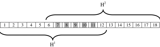
Let H1, . . . ,HL be a set of hypothesis spaces, each with a fitting learning algorithm, Al. Further suppose that the intersection of all hypothesis spaces is not empty and all learning algorithms are forced to agree and output the same hypothesis. Then

effec-tively the algorithms select a hypothesis from a smaller hypothesis space: L

l=1

Hl. If it

is further assumed that the hypothesis that best fits the training set belongs to every Hl (thus available to all algorithms), this scheme produces a hypothesis from a potentially much smaller hypothesis space which is just as good on the training sample. Hence, the generalization capability of such a hypothesis, as drawn from theorems such as The-orem 2, is potentially much better than the hypotheses outputted from any algorithm operating alone.

While the above discussion would yield the expected theoretical gain, it is very hard to implement. First, demanding that the algorithms output exactly the same hy-pothesis entails an ability that is unlikely to be easily available. Typically the different hypothesis spaces would consist of classifiers as different as neural networks and Bayes classifiers. The need to test (or construct) whether two classifiers are absolutely equal in functionality would render this scheme impractical. Existing algorithms could not be used as is, if at all, and would have to be thoroughly changed. Second, it is also unrealistic to demand that the hypothesis spaces will have an intersection which is rich enough to be useful to correctly classify different target distributions. While this might be feasible for L=2 (such as the assumption in [5]) it is highly unlikely for a bigger number of learners. A more relaxed agreement demand will now be presented, along with a simple way of checking it: unlabeled examples.

Definition 4.

1. Define the variance of a vector inRLto be:

V(y1, . . . ,yL) =1

L L

∑

l=1

yl2₋ 1 L

L

∑

l=1

yl

!2

.

2. Furthermore, define the variance of a set of classifiers f1_{, . . . ,f}L _{to be the} ex-pected variance on examples from

X

:

V f1, . . . ,fL=EV f1(x), . . . ,fL(x).

Definition 5. For anyν>0, define theν-intersection of a set of hypothesis spaces, H1_{, . . . ,H}L_{to be:}

ν−

L

l=1

Hl=nf1, . . . ,fL :_∀l, fl_∈Hl,and V(f1, . . . ,fL)≤νo.

In effect theν-intersection of H1, . . . ,HLcontains all the hypotheses whose differ-ence with some of the members of other hypothesis spaces is hard to discover. This relaxed definition of intersection will be used as the space from which the algorithms can draw their hypotheses. Note that for ν=0, the 0-intersection is precisely2 the normal intersection of H1, . . . ,HL.

As mentioned before, unlabeled examples will be used to measure the level of agreement between the various learners. Therefore, let U =uj nu_j=1 be a set of un-labeled examples, drawn independently from the same distribution P but without the label being available. It will now be shown that if enough unlabeled examples are drawn, the disagreement measured on them is a good representative of the global dis-agreement. This will be done by defining a new hypothesis space V(H1, . . . ,HL)and a target distribution ˜P and using a generalization bound resembling Theorem 2.

Definition 6.

1. Let V H1, . . . ,HL=V_◦ f1, . . . ,fL: f1_∈H1, . . . ,fL_∈HL where V_◦ f1_{, . . . ,f}l_:

_X

_{→[0,1]is defined by:}

V_◦ f1, . . . ,fL(x) =V f1(x), . . . ,fL(x).

2. Let ˜P be a probability distribution over

X

_×[0,∞]which is defined by:

(∀A_⊆

X

_×[0,∞])_P˜_{(A) =P({(x,y)∈}

_X

_×

_Y

_{:(x,0)∈A}).}

In essence, ˜P labels all examples in

X

with 0, while giving them same marginal probability as before.

Before we can use the generalizing bound, we need to establish the Rademacher complexity of the new hypothesis space V(H1, . . . ,HL). This will be done using the following theorem from [2] (Theorem 10) which gives some structural properties of the Rademacher complexity.

Theorem 7. Let F,F1, . . . ,Fkand H be classes of real functions. Then 1. If F_⊆H, Rn(F)≤Rn(H).

2. Rn(F) =Rn(convF)where

convF=

(

T

∑

t=1

αtft :∀t ft∈F andαt≥0, T

∑

t=1 αt=1

)

is the class of all finite convex combinations of functions from F.

2_{This assumes that no element inXhas zero marginal probability. In the case thatXcontains non-empty}

The Value of Agreement A New Boosting Algorithm

3. For every c_∈R, Rn(cF) =|c|Rn(F)where cF={c f : f∈F}.

4. Ifφ:R→Ris Lipschitz with a constant Lφand satisfiesφ(0) =0, then Rn(φ(F))≤ 2LφRn(F)whereφ(F) ={φ◦f : f∈F}.

5. Rn ∑ki=1Fi

≤∑k

i=1Rn(Fi)where∑ki=1Fi=

∑k

i=1fi :∀i fi∈Fi .

Note that clause 2 in Theorem 7 is what makes the Rademacher complexity so attractive in boosting. Since the complexity of all convex combinations of classifiers from a weak hypothesis space is the same as the complexity of the space it self, it results in good generalization bounds.

Corollary 8. Rn V H1, . . . ,HL

≤8 maxlRn Hl

.

Proof. The result will follow from the following fact:

V H1, . . . ,HL_⊆1 L

L

∑

l=1 φHl

+

"

−φ 1_L

L

∑

l=1

Hl

!#

whereφ(z) =z2and is Lipschitz on

Y

_⊆[−1,+1]with Lφ=2. Therefore, from Theorem 7

Rn V H1, . . . ,HL _≤ Rn 1 L

L

∑

l=1 φHl

+

"

−φ 1_L

L

∑

l=1 Hl !#! ≤ 1 L L

∑

l=1 Rn

φHl+Rn φ 1 L L

∑

l=1 Hl !!

≤ 1_L

L

∑

l=1

2LφRn

Hl

+2Lφ1

L L

∑

l=1 Rn Hl

≤ 8 max

l Rn

Hl

.

Before proving the main theorems of the section, the following generalization bound (adapted from [2]) is presented. This theorem allows the use of an arbitrary loss func-tion and does not use the concepts of margins.

Theorem 9. Consider a loss function

L

:

Y

_×R→[0,1]and let F be a class of func-tions mapping

X

to

Y

. Let_{(xi,yi)}ni=1be a sample independently selected according

to some probability measure P. Then, for any integer n and any 0<δ<1, with proba-bility of at least 1₋δover samples of length n, every f _∈F satisfies

EL(Y,f(X))≤Eˆn

L

(Y,f(X)) +Rn ˜L◦F

+

r

8 log(2/δ)

n

where ˆEnis the expectance measured on the samples and ˜

L_◦F={(x,y)7→

L

(y,f(x))−

L

(y,0) : f_∈F_}.

Theorem 10. Let H1_{, . . . ,H}L _{be sets of functions from}

_X

_to

_Y

_{and let U=u} j n_j=1 be a set of unlabeled examples drawn independently according to a distribution P over

X

_×

Y

. Then for any integer n and 0<δ<1, with probability of at least 1₋δevery set of functions fl_∈Hl, l=1. . .L satisfies:

V(f1, . . . ,fL)≤_Vˆ_(f1_{, . . . ,f}L_{) +8 max} l Rn(H

l_{) +}

r

8 log(2/δ)

n

where ˆV(f1, . . . ,fL)is the sampled expected variance, as measured on U=uj n j=1.

Proof. The theorem follows directly from Theorem 9 when applied to the function set V(H1, . . . ,HL)with ˜P as target distribution. The loss function is defined by

L

(y,z) =

min_{|y₋z_|,1_}. Since ˜P assigns zero probability to all non-zero labels,

EL Y,V f1(X), . . . ,fL(X)=EV f1(X), . . . ,fL(X)=V(f1, . . . ,fL)

and

ˆ

EL Y,V f1(X), . . . ,fL(X)=_Vˆ_(f1_{, . . . ,f}L_). Furthermore Rn ˜L◦F

=Rn V(H1, . . . ,HL)

since

˜

P

L

y,V_◦(f1, . . . ,fL)(x)−

L

(y,0)6=V_◦(f1, . . . ,fL)(x)=0.

Therefore, Theorem 9 implies that, with a probability of at least 1−δ,

V(f1, . . . ,fL) ≤ _Vˆ_(f1_{, . . . ,f}L_{) +Rn V(H}1_{, . . . ,H}L₎₊

r

8 log(2/δ)

n

≤ _Vˆ_(f1_{, . . . ,f}L_{) +8 max} l Rn(H

l_{) +}

r

8 log(2/δ)

n where the last inequality holds due to the corollary of Theorem 7.

Theorem 10 allows us to use a finite set of unlabeled examples to make sure (with high probability) that the classifiers selected by the learning algorithms are indeed in the desiredν-intersection of the hypothesis spaces. This allows us to adapt generaliza-tion bounds to use smaller hypothesis spaces. As an example, an adapted version of Theorem 2 is presented.

Theorem 11. Let H1, . . . ,HL be a class of real-valued functions from

X

to[−1,+1]

and letθ_∈[0,1]. Let P be a probability distribution on

X

_{× {−}1,+1_}and suppose that a sample of ns labeled examples S=

(xj,yj) ns_j=1 and nu unlabeled examples U =uj

nu

j=1is generated independently at random according to P. Then for any

integer ns,ν>0, 0<δ<1 and nusuch that 8 maxlRnu(Hl) +

q

8 log(4/δ)

nu ≤

ν

2, with a

probability at least 1₋δ, every f1_∈H1, . . . ,fL_∈HLwhose disagreement ˆV on U is at mostν₂satisfies

∀l P(y₆=sign(fl(x)))≤ˆLθ(fl) +

2Rns(ν−

ˆl

Hˆl)

θ +

s

log(4/δ)

2ns

where ˆLθ(fl_{) =} 1

ns ns

∑

j=1

I yifl(xi)≤θ

The Value of Agreement A New Boosting Algorithm

Proof. From Theorem 10, with a probability of at least 1₋δ₂, V(f1_{, . . .f}L_)≤ν_and therefore_∀l fl_∈v₋

ˆl

Hˆl. Applying Theorem 2 to v₋

ˆl

Hˆl, with a probability of at

least 1₋δ₂,

∀f _∈ν₋

ˆl

HˆlP(y₆=sign(f(x)))≤ˆLθ(f) +

2Rns(ν−

ˆl

Hˆl)

θ +

s

log(4/δ)

2ns

using the union bound and combining the results proves the theorem.

To conclude this section, we note that the proposed settings has the following desired property: it doesn’t help to have duplicate copies of the same hypothesis space. To have any advantage,ν₋

ˆl

Hˆlmust be considerably smaller then any of the base hypothesis

spaces. Therefore, using only duplicate copies of the same hypothesis space H =

H1, . . .HLgivesν₋

ˆl

Hˆl=H and hence no improvement. Furthermore, any duplicates

within the set of different hypothesis spaces can be removed without changing the results.

2.3

Reduction of labeled examples

The previous section presented a formal setting where agreement was used to reduce the complexity of the set of possible hypotheses. The immediate implication is that training error serves as a better approximation for global true error. Therefore, for a given number of labeled examples, if the learning algorithm has produced a classifier with a low training error one can expect a lower global error. However this reduction in complexity can be also viewed from a different, though very related, point of view.

Since most algorithms can reduce the training error to a very low level, the number of labeled examples necessary is usually determined as to decrease the two other terms in generalization bounds: the complexity of the hypothesis space and the certainty in the success of the whole procedure (δ). Using more labeled examples typically allows using a lowerδvalue without hindering the expected error of the resulting classifier (for example, Theorem 2 involves a

q

log(2/δ)

2N term). The second result of increasing

the number of labeled examples is reduction in the Rademacher complexity (or sim-ilar complexity terms). Therefore, decreasing the term relating to hypothesis space complexity, enables one to use less labeled examples while achieving the same bound. To illustrate this consider Blumer et al. result [6] concerning the simple case of consistent learners:

Theorem 12. (adapted from 2.1.ii in [6]) For anyε>0,δ>0, a probability distri-bution P over

X

and a hypothesis space H _{⊆ {−}1,+1_}X of finite VC dimension, d. Let ˆf _∈H be some target function and S= xj,fˆ(xj)

ns

j=1a sample independently

drawn from

X

where nsis larger than max

₄

εlog2δ,8dε log13ε . Then with probability

of at least 1₋δover samples of size ns, for any function f∈H which correctly classify all sampled examples, P(f(x)6=fˆ(x))<ε.

To prove the theorem, Blumer et al. showed that with high probability, a sample of size max4_εlog2_δ,8d

‘far’ from the target ˆf . If H is made smaller, the number of functions which need to be excluded is reduced. Therefore, less labeled examples are needed in order to exclude high error functions.

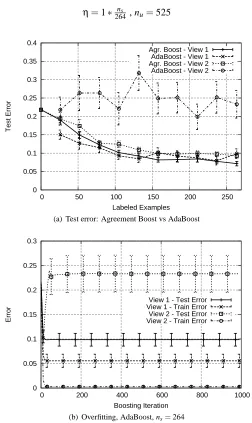
In many learning applications one often comes across a phenomena called over-fitting. In these cases, the learning algorithm produces a classifier which is overly trained on the training sample. The classifier is too specialized in classifying the learn-ing sample and looses its generalization powers. In other words, the algorithm learns information that is accidentally available in the training sample but is specific to it. For an iterative learning algorithm (improving its current classifier with every iteration), one typically observes a reduction in both training and test (global) error in the begin-ning of the algorithm’s run. However, from some point on, the test error will start to increase, while the training error is still being reduced[21, 22].

Chapter 3

The Algorithm

In this chapter, we propose a new boosting algorithm named AgreementBoost (Algo-rithm 3), which exploits the benefits suggested by the theory presented in the previous chapter. Like AdaBoost, the algorithm is designed to operate in Boolean scenarios where each example can belong to one of two possible classes denoted by_±1 (i.e.,

Y

={+1,−1_}).

As in many boosting algorithms, AgreementBoost creates combined classifiers or ensembles. However, instead of just one such classifier, AgreementBoost creates L ensembles, one for each hypothesis space. The ensembles are constructed using L un-derlying learning algorithms, one for each of the L hypothesis spacesHl L

l=1. At each

iteration, one of the learning algorithms is presented with a weighing of both labeled and unlabeled examples in the form of a weight vector w(x)and pseudo-labels for the unlabeled examples (y(u)). The underlying learner is then expected to return a hypothe-sis f_tl with a near-optimal1edge2:γ= ∑

(xj,yj)∈S

w(xj)yjfl(xj) + ∑ uj∈U

w(uj)y(uj)fl(uj).

The returned hypothesis is then added to the corresponding ensemble. The weight given to f_tl(α_tl, selected at step 2.a.iii) is chosen such that the cost function F is mini-mized. This can be done by any numeric line minimization algorithm.

The proposed AgreementBoost can be described as a particular instance of Any-Boost [21], a boosting algorithm allowing for arbitrary cost functions. Agreement-Boost’s cost function F has been chosen to incorporate the ensembles’ disagreement into the normal margin terms. This is achieved using a weighted sum of two terms: an error or margin-related term (∑L_l=1∑ns_j=1er ₋yjgl(xj)

) and a disagreement term

∑nu

j=1er(V(uj)). Despite of the fact that the these terms capture different notions, they are very similar. Both terms use the same underlying function, er(x), to assign a cost to some example-related measure: The first penalizes low (negative) margins while the second condemns high variance (and hence disagreement). AgreementBoost allows choosing any function as er(x), so long as it is convex and strictly increasing. This freedom allows using different cost schemes and thus for future cost function analysis (as done, for example, in [21]). In the degenerate case where no unlabeled examples are used (nu=0) and exis used as er(x), AgreementBoost is equivalent to L independent

1_{For the exact definition of ‘near-optimal’, see Chapter 4.}

2_{Note that the edge can be rewritten in terms of the weighted error of f}l _{:γ=1−2ε whereε=}

∑

(xj,yj)∈S

w(xj)Iyj=6 fl(xj)+ ∑ uj∈U

w(uj)Iy(uj)6=fl(uj). Therefore fl having a near-optimal edge is

Algorithm 3 Agreement Boost

Denote F g1, . . . ,gL=∑L

l=1∑nsj=1er −yjgl(xj)

+ηL∑nu_j=1er(V(uj))where

V(u) =1

L L

∑

l=1

gl(u)2₋

1

L L

∑

l=1

gl(u)

2

,η_∈R+is some positive real number and er :R→Ris some convex, strictly increasing function with continuous second derivative.

1. Set gl_≡0 for l=1. . .L. 2. Iterate until done (counter t):

(a) Iterate over l=1. . .L:

i. Set w(xj) =er0 −yjgl(xj)

yj/Z for all(xj,yj)∈S and w(uj) =2η

L1∑

L

ˆl=1g ˆl_(u

j)−gl(uj)

er0(V(uj))/Z for all uj∈U where Z is a renormalization factor s.t.∑

xj

w(xj) +∑ uj

w(uj) =1.

Use y(uj) =sign

1

L∑ L

ˆl=1g ˆl_(u

j)−gl(uj)

as pseudo-labels for uj.

ii. Receive hypothesis fl

t from learner l using the above weights and labels.

iii. Findα_tl_≥0 that minimizes F g1, . . . ,gl+αl

tftl, . . . ,gL

.

iv. Set gl=gl+αl tftl.

3. Output classifier sign(gl)whose error on the samples is minimal out of the L classifiers.

Chapter 4

Proof of convergence

In this chapter a convergence proof for Algorithm 3 is given. The proof considers two scenarios. The first assumes that the intersection of all conv Hlis able to correctly classify all labeled examples using classifiers which agree on all unlabeled examples. Under this assumption, it is shown that the algorithm will produce classifiers, which in the limit are fully correct and agree on all unlabeled examples. In other cases, where this assumption is not valid, the algorithm will produce ensembles which minimize a function representing a compromise between correctness and agreement.

Both Mason et al. [21] and Rätsch et al. [24] provide similar convergence proofs for AnyBoost-like algorithms. While both proofs can be used (with minor modifications) in our settings, they do not fully cover both scenarios. The proof in [24] demands that the sum of theαl

t coefficients will be bounded and thus cannot be used in cases where the theoretical assumptions hold. This can be seen easily in the case of AdaBoost, where a fully correct hypothesis will be assigned an infinite weight. While Agreement-Boost will never assign an infinite weight to a hypotheses (due to the disagreement term), it is easy to come up with a similar scenario where the coefficient sum grows to infinity. In [21], Mason et al. present a theorem very similar to Theorem 18 below. However, they assume that the underlying learner performs perfectly and always re-turns the best hypothesis from the hypothesis space. Such a severe assumption is not needed in the proof presented here. Furthermore, due to the generality of AnyBoost, the result in [21] apply to the cost function alone and is not translated back to training error terms.

The proofs below are based on two assumptions concerning the learning algorithms and the hypothesis spaces. It is assumed that when presented with an example set1S and a weighing w(x), the underlying learning algorithms return a hypothesis fl _for which:

∑

(xj,yj)∈S

w(xj)yjfl(xi)≥δmax

ˆ

f∈Hl

∑

xj∈S

w(xj)yjfˆ(xi)

!

for someδ>0.

The second assumption concerns the hypothesis spaces: it is assumed2that for every l and some fl_∈Hlthe negation of flis also in Hli.e.: f _∈Hl_{⇒ −}f_∈Hl. This allows

1_{Note that this may include examples labeled by the algorithm, rather the being drawn according to the}

underlying distribution P.

2_{Note that this is assumed for simplicity alone. By allowing the algorithm to use negative values forα}l t

all hypothesis spaces become Hl_{∪ −H}l_{, which are closed under negation. This inflicts no increase in the}

us to using absolute value in the previous assumption:

∑

xj∈S

w(xj)yjfl(xj)≥δmax

ˆ

f_∈Hl

x

∑

j∈S

w(xj)yjfˆ(xi)

for someδ>0.

In the Lemmas and Theorems to follow, it will sometimes be assumed that the hypothesis spaces are finite. Due to the fact that there is only finite amount of ways to classify a finite set of examples with a_±1 label, if some of the hypothesis spaces are infinite it will be indistinguishable when restricted to S and U . Therefore, without loss of generality, one can assume that the number of hypotheses is finite.

The convergence of the algorithm is proven taking a different point of view to the ensembles built by the algorithm. The ensembles can be seen as a mix of all possible functions in the hypothesis spaces rather then as an accumulation of hypotheses:

Definition 13.

1. Let Hl=f_il _i

∈Il be an enumeration of functions in H

l_{. One can rewrite the}

en-sembles glbuilt by AgreementBoost as functions from X_×R|Hl|toR: gl(x,βl_{) =}

∑

i

βl

ifil(x) for βl = βl1,βl2, . . .

∈R|Hl| and l =1. . .L. Further denote β=

β1_{, . . . ,}βL_{. Note that} βl

i is the sum of all αlt chosen by the algorithm such that f_tl_≡f_il.

2. Let the variance of g1, . . . ,gLon an example u be

V(u,β) = 1

L L

∑

l=1

gl(u,βl)2−

" 1 L L

∑

l=1

gl(u,βl)

#2

.

3. Whenever it is clear from context what are theβparameters, V(u)and gl(u)will be used for brevity.

4. Let er :R→R+be a convex monotonically increasing function. Denote by

F(β) = E(β) +ηD(β)

E(β) =

L

∑

l=1 ns

∑

j=1 er

−yjgl(xj)

(4.1)

D(β) = L

nu

∑

j=1

er(V(uj))

for someη>0.

F(β)represents a weighing between correctness and disagreement. E(β), being a sum of loss functions penalizing negative margins, relates to the current error of the ensemble classifiers. D(β)captures the ensembles’ disagreement over the unlabeled examples.

Using the above notations and the new point of view, the margins of hypotheses becomes proportional to the partial derivative of F(β)with respect to the corresponding

The Value of Agreement A New Boosting Algorithm

coefficient. Replacing the examples’ weight and labels according to the definition of AgreementBoost, we have that:

∑

xj∈S

w(xj)yjfil(xj) + ∑ uj∈U

w(u)y(uj)fil(uj) =

1

Z ∑ xj∈S

er0 ₋yjgl(xj)

yjfil(xj) +

2η

Z ∑

uj∈U

er0(V(uj))

1

L∑ L

ˆl=1gˆl(uj)−gl(uj)

fl i(uj)

=−1

Z

∂F

∂βl i

(β.)

Therefore the underlying learners return hypotheses whose corresponding partial deriv-atives maintain the following inequality:

−_∂β∂F_l

i

(β)≥δmax

ˆi − ∂F

∂βl

ˆi

(β).

Furthermore, since the hypothesis spaces are assumed to be closed under negation, the following holds as well:

−_∂β∂F_l

i

(β)≥δmax

ˆi − ∂F

∂βl

ˆi

(β) =δmax

ˆi ∂F ∂βl ˆi

(β)

.

Note that this ensures that the partial derivative with respect to the returned function coefficient is non-positive and hence the choice ofαl_t in step 2.a.ii of Algorithm 3 is in fact the global optimum3over allR. Since in every iteration only one coefficient is changed to a value which minimizes F(β), Algorithm 3 is equivalent to a coordinate descent minimization algorithm (for more information about minimization algorithms see, for example, [9]).

As a last preparation before the convergence proof, it will be shown that F(β)is convex. Apart from having other technical advantages, this guaranties that the algo-rithm will not get stuck in a local minimum:

Claim 14.

1. _∀u_∈U , er(V(u,β))is convex with respect toβ. 2. _∀xj∈X , er(−yjgl(xj,βl))is convex with respect toβl. Proof. The claim will follow from the following facts:

1. The operator g(β) = g1(β1_{), . . . ,g}L_(βL_{)is linear. Therefore, for everyβ, ˆβand}

∀α,γ∈[0,1], we have that g(αβ+γβˆ) =αg(β) +γg(βˆ).

2. Let A,B_∈RLbe two vectors andα,γ∈[0,1]two numbers such that α+γ=1. Further denote the variance of a vector v= (v1, . . . ,vL) by V(v) = 1_L

L

∑

i=1

v2_{i −}

1 L2 _L ∑ i=1 vi 2

. Then the following holds:

V(αA+γB) = α2_{V(A) +γ}2_{V(B) +2αγcov(A,B)} ≤ α2V(A) +γ2V(B) +αγ(V(A) +V(B)) = αV(A) +γV(B)

where cov(A,B)is the covariance of the two vectors and is defined in a similar fashion to V(v).

3. _∀c_∈Rthe function er(cx)is convex with respect to x.

4. er is monotonically increasing.

Therefore, for everyβ, ˆβand_∀α,γ∈[0,1]such thatα+γ=1, using fact 1 and fact 2 above, we have that V(u,αβ+γβˆ)≤αV(u,β) +γV(u,βˆ). Using fact no. 4 and er’s convexity, we have that

er

V(u,αβ+γβˆ)≤er

αV(u,β) +γV(u,βˆ)≤αer(V(u,β)) +γer

V(u,βˆ)

proving the first part of the claim.

For the second part, Facts 1 and 3 are used together, giving that

er(−yjgl(xj,αβl+γβˆl)) = er

−yj

h

αgl(xj,βl) +γgl(xj,βˆl)i

≤ αer₋yjgl(xj,βl)

+γer₋yjgl(xj,βˆl)

proving the second part of the claim.

Lemma 15. The function F(β)is convex with respect toβ.

Proof. This follows immediately from Claim 14 and the fact that a sum of convex functions is convex.

Lemma 16. Let_{βn}be a sequence of points generated by an iterative linear search algorithm A, i.e., βn+1=A(βn)minimizing a non-negative convex function4F∈C2. Denote the direction in which the algorithm minimizes F in every step by vn=_kββn+1−βn

n+1−βnk_∞ and Fn(α) =F(βn+αvn)(i.e., A minimizes Fn(α)in every iteration by a linear search). Then, if_∃M_∈R+such that_∀n d2Fn

dα2(α)≤M for every ‘feasible’α(i.e., when Fn(α)≤

F(βn)) then lim n→∞

dFn

dα(0) =0.

Proof. By Taylor expansion Fn(α) =Fn(0) +Fn0(0)α+ Fn00(ξ)

2 α2for someξbetween 0

andα. Therefore Fn(0)−Fn(α) =−Fn0(0)α− Fn00(ξ)

2 α2≥ −Fn0(0)α−12Mα2since by

assumption d2Fn

dα2(ξ)≤M (by the convexity of F, ifαis feasible, all points between it

and 0 are also feasible). From the previous inequalities it follows that

F(βn)−F(βn+1) = F(βn)− min

f easibleαFn(α) =f easiblemaxα(Fn(0)−Fn(α))

≥ max f easibleα

−F_n0(0)α−1₂Mα2

= max

α∈R

−F_n0(0)α−1₂Mα2

=Fn0(0)

2

2M ≥0.

Note that the last inequality ensures that the last expression is maximized by a feasible

α, making the equality argument valid.

Now, since F(βn)is a monotonically decreasing sequence and is bounded from below, it must converge. Therefore lim

n→∞(F(βn)−F(βn+1)) =0, which together with the above inequality, gives the result.

The Value of Agreement A New Boosting Algorithm

Lemma 17. Let_{βn}be a sequence of points generated by an iterative linear search algorithm A (i.e.,βn+1=A(βn)) minimizing a non-negative convex function F∈C2. If in addition to the conditions of Lemma 16 (and using the same notations),_∃m>0_∈

R such that_∀n d2Fn

dα2(α)≥m for every ‘feasible’α (i.e., when Fn(α)≤F(βn)) then

lim

n→∞kβn+1−βnk∞=0.

Proof. The proof is similar to the one of Lemma 16. By Taylor expansion Fn(α) =Fn(0) +Fn0(0)α+

Fn00(ξ)

2 α2for someξbetween 0 andα.

Therefore Fn(0)−Fn(α) =−Fn0(0)α− Fn00(ξ)

2 α2≤ −Fn0(0)α−12mα2since by

assump-tiond_d2_αFn2(ξ)≥m. It follows that for theαchosen at step n,|α|must be smaller or equal

to 2Fn0(0)

m

. By Lemma 16 lim n_→∞F

0

n(0) =0, and therefore kβn+1−βnk∞=kαvnk∞=

|α| −→0.

Theorem 18. For some non-empty sets of labeled examples S and unlabeled

exam-ples U , suppose that the underlying learners are guaranteed to return a hypothesis ˆf

such that∑ x

w(x)yxfˆ(x)≥δ

max f

∑_xw(x)yxf(x)

for some constantδ>0 and every weighing w(x)of their examples. Further let er :R→R+be a non constant convex monotonically increasing function such that:

1. er_∈C2and er0(0)>0.

2. _∃M_∈R+for which er(x)≤max n

L(|S_|+η|U_|)er(0),1

η(|S|+η|U|)er(0)

o

im-plies that er00(x)<M.

Then it holds that lim

n→∞k∇F(βn)k∞=0.

Proof. Since Algorithm 3 is equivalent to performing a coordinate descent which min-imizes

F(β) =

∑

l

∑

xi

er(−yigl(xi)) +ηL

∑

uj

er(V(uj))

the result will follow from Lemma 16 and Lemma 17.

Using the same notation as in Lemma 16, one must show that_∀n d2Fn

dα2(α)≤M0for

every ‘feasible’αand some M0_∈R+. Since Algorithm 3 only changes one coordinate at a time, it is enough to show that the second derivative with respect to each coordinate is bounded.

∂2_F ∂βl

i∂βli

=

∑

xj∈S er00

−yjgl(xj)

h

yjfil(xj)

i2

+4η L_uj

∑

_∈Uer

00_(V(u

j))

" 1

L

∑

ˆl

gˆl(uj)−gl(uj)

#2

f_il(uj)2 (4.2)

+2η

∑

uj∈U

er0(V(uj)) L₋1

L f

l i(uj)2.

Denote Lη=maxnL,1

η

o

andξ=sup_{x : er(x)≤Lη(|S_|+η|U_|)er(0)}(note that er convexity and the fact that it is not a constant function imply that lim

x→∞er(x) =∞

monotonically increasing. Hence it holds that er(x)≤L_η(|S_|+η|U_|)er(0) implies er0(x)≤er0(ξ). Therefore, without loss of generality, we can assume that er(x)≤

L_η(|S_|+η|U_|)er(0)implies that both er0(x)and er00(x)are bounded by M.

Let_{βn}be the sequence of coefficient vectors generated by Algorithm 3. Since

β0 is the all zero vector, F(β0) =L(|S_|+η|U_|)er(0). Therefore for every ‘feasi-ble’ β which the algorithm might consider, it must hold that F(β)≤F(β0). Since

(∀x) [er(x)≥0], this implies that

(∀l,j)her(−yjgl(xj))≤L(|S_|+η|U_|)er(0)i

and

(∀j)

er(V(uj))≤ 1

η(|S|+η|U|)er(0)

. Therefore, " 1 L

∑

ˆl

gˆl(uj)−gl(uj)

#2

≤LV(u)≤Lξ. (4.3)

From which it follows that for every feasibleβ:

∂2_F ∂βl

i∂βli

(β) ≤

∑

xj∈S

Mhyjfil(xj)

i2

+4η

L_uj

∑

_∈UMLξf l

i(x)2 (4.4)

+2η

∑

uj∈U

ML−1

L f

l i(x)2

≤ M(|S_|+2η_|U_|(2ξ+1)),

where the last inequality follows from the fact that yj,fil(xj)∈ {−1,1}. This completes the necessary requirements of Lemma 16 and therefore lim

n→∞

∂F

∂βln in

=0 where lnand in

are the indices of the hypothesis returned by the underlying learner at iteration n. By the assumptions regarding the base learners and the hypothesis spaces

−∂F ∂βln

in

≥δmax i −

∂F

∂βln i

=δmax i ∂F ∂βln i

giving that_∀i_∈Iln lim n→∞ ∂β∂Fln

i

(βn)

=0.

Since in Algorithm 3, ln= (n mod L) +1, in order to complete the proof it is

enough to show that_∀ˆl=1. . .L,_∀i_∈I_lnb lim n_→∞

_∂β∂Flnb

i

(βn)

=0 wherelbn= n+ˆl mod L

+

1. Using the above as base for an induction argument (for ˆl=L), it is enough to show that if the claim holds for ˆl+1, it also holds for ˆl. Let i be some index in I_lnb. By the inductive assumption, it holds that

lim n→∞ ∂F

∂βlnb i

(βn−1)

=0 (note thatlbn= n−1+ˆl+1 mod L

[image:29.595.116.471.97.357.2]

The Value of Agreement A New Boosting Algorithm

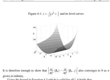
Figure 4.1: z=√1_yx2+1_y and its level curves

It is therefore enough to show that _∂β∂Flnb

i

(βn)− ∂F

∂βlnb i

(βn−1)

also converges to 0 as n grows to infinity.

Using the bound in Equation 4.3 which is valid for all l, it holds that

∀l 1 L

∑

ˆl

gˆl(uj)−gl(uj)

≤ p Lξ

for all ‘feasible’βand therefore for allβbetweenβn₋1andβn. Denoting again by in₋1

the function index returned by learner ln₋1in iteration n−1, one can show in a very

similar way to that used to develop Equation 4.4 that

∂2_F ∂βln−1

in−1∂β

b ln i

(β)

≤

M(|S_|+2η_|U_|(2ξ+1)) (4.5)

for allβbetweenβn−1andβn, regardless to whether ln−1=lbnor not.

From Equation 4.5, sinceβnandβn−1differ in only one coordinate, it follows that

∂F

∂βlnb i

(βn)−

∂F

∂βlnb i

(βn−1)

≤M(|S|+2η|U|(2ξ+1))kβn−βn−1k∞. Furthermore, since er0(V(u))≥er0(0), it follows from Equation 4.2 that

∂2_F ∂βl

i∂βli

≥2ηL−1 L |U|er

0₍₀₎

allowing to invoke Lemma 17 and conclude the proof.