Version: Accepted Version
Article:
Hamilton, J. orcid.org/0000-0003-3326-9842, Nunes, M.A., Knight, M.I. et al. (1 more author) (2017) Complex-valued wavelet lifting and applications. Technometrics. ISSN 0040-1706
https://doi.org/10.1080/00401706.2017.1281846
Reuse
Items deposited in White Rose Research Online are protected by copyright, with all rights reserved unless indicated otherwise. They may be downloaded and/or printed for private study, or other acts as permitted by national copyright laws. The publisher or other rights holders may allow further reproduction and re-use of the full text version. This is indicated by the licence information on the White Rose Research Online record for the item.
Takedown
If you consider content in White Rose Research Online to be in breach of UK law, please notify us by
Complex-valued wavelet lifting and applications
Jean Hamilton
HEDS, ScHARR, University of She
ffi
eld
Matthew A. Nunes
∗Department of Mathematics and Statistics, Lancaster University
Marina I. Knight
Department of Mathematics, University of York
and
Piotr Fryzlewicz
Department of Statistics, London School of Economics
Abstract
Signals with irregular sampling structures arise naturally in many fields. In applications such as spectral decomposition and nonparametric regression, classical methods often assume a regular sampling pattern, thus cannot be applied without prior data processing. This work proposes new complex-valued analysis techniques based on the wavelet lifting scheme that removes ‘one coefficient at a time’. Our proposed lifting transform can be applied directly to irregularly sampled data and is able to adapt to the signal(s)’ characteristics. As our new lifting scheme produces complex-valued wavelet coefficients, it provides an alternative to the Fourier transform for irregular designs, allowing phase or directional information to be represented. We discuss applications in bivariate time series analysis, where the complex-valued lifting construction allows for coherence and phase quantification. We also demonstrate the potential of this flexible methodology over real-valued analysis in the nonparametric regression context.
Keywords: lifting scheme; wavelets; nondecimated transform; (bivariate) time series; coherence
and phase; nonparametric regression.
1
Introduction
Since the early nineties, wavelets have become a popular tool for nonparametric regression,
sta-tistical image processing and time series analysis. In particular, due to their natural localisation,
wavelets can provide sparse representations for certain functions that cannot be represented effi
-ciently using Fourier sinusoids. Reviews of the use of wavelets in statistics include Nason (2008)
and Abramovich et al. (2000).
Until recently, the majority of work in the statistical literature has been based on the discrete
wavelet transform (DWT). However, classical wavelet methods suffer from some limitations; in
particular, usage is restricted to data sampled at regular time or spatial locations, and a dyadic data
dimension is often imposed. Wavelet lifting (Sweldens, 1996) can be used to overcome many of the
shortcomings of the standard DWT. Specifically, wavelet functions obtained through the wavelet
lifting scheme provide an extension of classical wavelet methods to more general settings, such as
irregularly sampled data.
On the other hand, it is now well-established that complvalued data analysis tools can
ex-tract useful information that is potentially missed when using traditional real-valued wavelet
tech-niques, even for real-valued data, see for example Lina and Mayrand (1995); Fernandes et al.
(2003); Selesnick et al. (2005). In particular, using complex-valued multiscale methods has been
advantageous in a range of statistical applications such as nonparametric regression (Barber and
Nason, 2004), image processing (Kingsbury, 1999; Portilla and Simoncelli, 2000) and time series
analysis (Magarey and Kingsbury, 1998; Kingsbury, 2001).
Complex-valued multiscale techniques building upon the lifting scheme as introduced by Sweldens
(1996) have been introduced in the literature by Abbas and Tran (2006), who briefly investigated
their proposed technique in the image denoising context, and by Shui et al. (2003), who focused
on the design of complex filters with desired band-pass properties.
This article introduces a new adaptive complex-valued wavelet lifting scheme built upon the
lifting ‘one coefficient at a time’ (LOCAAT) framework of Jansen et al. (2001, 2009). A
nondeci-mated variant of the proposed transform, which allows for an overcomplete representation of such
ap-through the complex-valued wavelet coefficients, the scheme exploits additional signal information not used by real-valued transforms; and (iii) applicability – it allows for the analysis of bivariate
nonstationary signals with possibly different (irregular) sampling structures, previously not directly
possible using methods currently in the literature.
We demonstrate the benefits of our new technique for spectral estimation of irregularly sampled
time series, with a particular focus on coherence and phase quantification for irregularly sampled
bivariate time series. In this context, the methodology can be viewed as a wavelet lifting analogue
to the Fourier transform and can be used for the same purposes. The good performance of our
method is also displayed in the nonparametric regression setting.
The paper is organised as follows. Section 2 introduces the new complex-valued lifting
algo-rithm, including its overcomplete variant. Section 3 details the application of the complex-valued
lifting algorithm to discover local frequency content of irregularly sampled uni- and bivariate time
series. Section 4 tackles nonparametric regression for (real-valued) signals.
2
The complex-valued lifting scheme
The lifting scheme (Sweldens, 1996) was introduced as a flexible way of providing wavelet-like
transforms for irregular data. Lifting bases are naturally compactly supported, and via the recursive
nature of the transform, one can build wavelets with desired properties, such as vanishing moments.
In addition, lifting algorithms are known to be computationally faster than traditional wavelet
transforms since they require fewer computations compared with classical transforms. For an
overview of the lifting scheme, see Schr¨oder and Sweldens (1996) or Jansen and Oonincx (2005).
In this section we introduce a complex-valued lifting scheme for analysing irregularly sampled
signals. The proposed lifting scheme can be thought of as a wavelet lifting analogue to the Fourier
transform. An irregularly sampled signal is decomposed into a set of complex-valued wavelet (or
detail) coefficients, representing the variation in the data as a function of location and wavelet scale
(comparable to Fourier frequency).
In a nutshell, the scheme can be conceptualised in two branches: one branch of the
imaginary component. Hence by using two different (real-valued) lifting schemes, one obtains a complex-valued decomposition, akin to the dual-tree complex wavelet transform of Kingsbury
(2001). However, our approach differs from that of Kingsbury (2001) in that it employs two lifting
schemes linked through orthogonal prediction filters, rather than two separate DWTs. The new
scheme is therefore able to extract information from signals via the two filters whilst also
natu-rally coping with the irregularity of the observations. Our approach also differs fundamentally
from the complex-valued lifting techniques currently in the literature (Abbas and Tran, 2006; Shui
et al., 2003) through the particular filter construction we propose (Section 2.2) in conjunction with
the lifting construction that removes ‘one coefficient at a time’ (Section 2.1). This allows us to
embed adaptivity in our complex-valued multiscale setup, i.e. construct wavelet functions whose
smoothness adjusts to the local properties of the signal.
In what follows we introduce the proposed scheme using an abstract choice of real and
imag-inary filters, and the subject of filter choice is deferred until Section 2.2, while an overcomplete
version of the complex-valued lifting transform is introduced in Section 2.3.
2.1
The algorithm
Suppose a function f (∙) is observed at a set of n irregularly spaced locations, x = (x1, . . . ,xn).
The proposed lifting scheme aims to decompose the data collected over the irregularly sampled
grid, {(xi, fi = f (xi))}ni=1, into a set of R smooth coefficients and (n − R) complex-valued detail
coefficients, with R the desired resolution level. The quantity R is akin to the primary resolution
level in classical wavelet transforms, see Hall and Patil (1996) for more details.
We propose to construct a new complex-valued transform that builds upon the LOCAAT paradigm
of Jansen et al. (2001, 2009), shown to efficiently represent local signal features in the fields of
non-parametric regression (Nunes et al., 2006; Knight and Nason, 2009) and spectral estimation (Knight
et al., 2012). We shall therefore refer to our proposed algorithm under the acronymC-LOCAAT.
Similar to the real-valued LOCAAT algorithm, C-LOCAAT can be described by recursively
applying three steps: split, predict and update, which we detail below. At the first stage (n) of the
algorithm, the smooth coefficients are set as cn,k = fk, the set of indices of smooth coefficients is
described using the distance between neighbouring observations, and at stage n we define the span
of xk as sn,k = xk+1−2xk−1. The sampling irregularity is intrinsically linked to the notion of wavelet
scale, which in this context becomes continuous, as opposed to dyadic in the classical wavelet
settings; this results in each coefficient having an associated scale across a continuum. This aspect
will be discussed in detail following the introduction of theC-LOCAAT algorithm.
In the split step, a point jn to be lifted is chosen. Typically, points from the densest sampled
regions are removed first, but other predefined removal choices are also possible (see Section 2.3).
We shall often refer to the removal order as a trajectory.
In the predict step the set of neighbours (Jn) of the point jnare identified and used to estimate
the value of the function at the selected point jn. In contrast to real-valued LOCAAT algorithms,
this is achieved using two prediction schemes, each defined by its respective filters, L and M. The
filter L corresponds to estimation via regression over the neighbourhood, as is usual in LOCAAT.
In order to extract further information from the signal, our proposal is to construct the second
filter (M) orthogonal on L, to ensure that it exploits further local signal information to the filter L.
Section 2.2 discusses this in detail.
The prediction residuals from using the two filters are given by
λjn = l
n jncn,jn −
X
i∈Jn
lnicn,i, (1)
μjn = m
n jncn,jn −
X
i∈Jn
mnicn,i, (2)
where{ln
i}i∈Jn∪{jn}and{m
n
i}i∈Jn∪{jn}are the prediction weights associated with L and M.
The complex-valued detail (wavelet) coefficient we propose is obtained by combining the two
prediction residuals
djn =λjn +iμjn. (3)
In the update step, the smooth coefficients{cn,i}i∈Jn and spans of the neighbours{sn,i}i∈Jn are updated
according to filter L:
cn−1,i = cn,i+bniλjn,
where bi are update weights. In practice, the update weights are chosen such that the mean of
the series is preserved throughout the transform, thus preserving the characteristics of the original
series (Jansen et al., 2009). One such choice is to set bni = (sn,jnsn−1,i)/(
P
i∈Jn s
2
n−1,i). The neighbours’
spans update accounts for the modification to the sampling grid induced by removing one of the
observations. Updating according to the L filter only ensures that there is a unique coarsening of
the signal for both the real and imaginary parts of the transform.
The observation jn is then removed from the set of smooth coefficients, hence after the first
algorithm iteration, the index set of smooth and detail coefficients are Sn−1 = Sn\{jn}and Dn−1 =
{jn} respectively. The algorithm is then iterated until the desired primary resolution level R has
been achieved. In practice, the choice of the primary level R in LOCAAT lifting schemes is not
crucial provided it is sufficiently low (Jansen et al., 2009), with R = 2 recommended by Nunes
et al. (2006).
After observations jn, jn−1, . . . , jR+1 have been removed, the function can be represented as a
set of R smooth coefficients,{cr−1,i}i∈SR, and (n−R) detail coefficients,{dk}k∈DR (DR = {jn, ..., jR+1}).
As in classical wavelet decompositions, the detail coefficients represent the high frequency
com-ponents of f (∙), whilst the smooth coefficients capture the low frequency content in the data.
The lifting scheme can be easily inverted by recursively ‘undoing’ the update, predict and
split steps described above for the first filter. Specifically, the update step is first inverted: cn,i =
cn−1,i−bniλjn, ∀i∈Jn, then the predict step is inverted by
cn,jn =
λjn −
P
i∈Jnl
n icn,i ln
jn
or (5)
cn,jn =
μjn −
P
i∈Jnm
n icn,i mn
jn
. (6)
Undoing either predict (5) or (6) step is sufficient for inversion. As for real-valued lifting,
inversion can also be performed via matrix calculations due to the transform linearity. However,
using (5) for inversion is generally computationally faster, especially for large n.
Wavelet lifting scales. The notion of wavelet scale in this context becomes continuous and is
intrinsically linked to the data sampling structure and trajectory (removal order) choice. Denote
lowα-values corresponding to fine scales. In order to give lifting scales a similar interpretation to
the classical notion of dyadic wavelet scale, we group wavelet functions of similar α-scales into
discrete artificial levels {ℓi}J
∗
i=1, as proposed by Jansen et al. (2009), for a chosen J∗. The further
use of artificial scales is discussed in Sections 2.3 and 3 (under the spectral estimation context)
and in Appendix B (under the nonparametric regression context). Note that the usage of the same
lifting trajectory for the two lifting branches (coupled with the one filter update) ensures that our
proposed lifting transform generates a common scale for both real and imaginary parts. In other
words, at each stage of the algorithm there is just one set of smooth coefficients associated to a
unique set of scales.
2.2
Filter construction
The proposed complex-valued lifting transform is illustrated schematically in Figure 1 in terms of
two general prediction filters L and M. As already explained, we construct the second filter (M)
orthogonal on L, thus ensure different signal content extraction.
For clarity of exposition, let us consider a LOCAAT scheme with a prediction step based upon
two neighbours in a symmetrical configuration. The regression over the neighbourhood generates
prediction weights for the two neighbours, let us denote them by l1and l3 (see equation (1)); this
prediction step can also be viewed as using a three-tap prediction filter (L) of the form (l1,1,l3),
which depends on the sampling of the observations x = (x1, . . . ,xn) (Nunes et al., 2006). We
determine the unique (up to proportionality) three-tap filter M that is orthogonal on L and ensures
at least one vanishing moment. Hence we can express the set of filter pairs as having the form
L = (l1,1,l3), l1,l3 >0
M = (m1,m2,m3),
and l1m1+m2+l3m3= 0 (i.e. L∙M=0) and l1+l3= 1, m1+m3= m2(i.e. ensure one vanishing
moment). The solution to these constraints can be parameterised as M = (−1+l3
1+l1m,
l1−l3
1+l1m,m). The
proportionality constant can be determined by bringing both filters L and M to the same scale
through kLk = kMk, which yields m = l1√+1
3. Hence the solution can be succinctly written as
M = (Am,(1+ A)m,m) with A = l1−2
l1+1 and m =
l1+1 √
L represents a prediction scheme using linear regression with two neighbours in a symmetrical
configuration. This is a choice that has proved to be successful both for (real-valued) nonparametric
regression (Nunes et al., 2006; Knight and Nason, 2009) and for (real-valued) spectral estimation
(Knight et al., 2012).
Since L can be viewed as a prediction filter for a real-valued LOCAAT scheme, we can also
employ the adaptive prediction filter choice of Nunes et al. (2006) in our proposed construction.
The ‘best’ local regression (order and neighbourhood) is chosen at each predict step, subject to
yielding minimising the detail coefficients. Consequently, we obtain an adaptive complex-valued
lifting transform, with the highly desirable flexibility of being able to adapt to the local
charac-teristics of the data – see Appendix B in the supplementary material for an illustration of this
adaptiveness in the nonparametric regression setting.
The orthogonality of the two filters M and L also mirrors the attractive properties of Fourier
sinusoids, hence this choice results in an interpretable quantification of phase, which shall further
be exploited according to the context—by phase alteration when denoising real-valued signals, or
by ensuring phase preservation in the context of spectral estimation.
A further insight and justification of the proposed filter choice is provided in Appendix C in
the context of coherence and phase estimation.
2.3
The nondecimated complex-valued lifting transform
In the classical wavelet literature, the nondecimated wavelet transform (NDWT) (Nason and
Silver-man, 1995) has properties that make it a better choice than the discrete wavelet transform (DWT)
for certain classes of problems, see e.g. Percival and Walden (2006). The concept is akin to basis
averaging, and has delivered successful results in both nonparametric regression and spectral
esti-mation problems, not only in the classical wavelet setting (NDWT) but also for irregularly spaced
data through the nondecimated lifting transform (NLT) (Knight and Nason, 2009; Knight et al.,
2012).
In this section, we also exploit the benefits of this nondecimation paradigm for irregularly
sampled data and to this end, we shall introduce the complex-valued nondecimated lifting
NDWT. Specifically, due to the irregular sampling structure, nondecimation cannot be performed
via decomposing shifts of input data without data interpolation.
Although similar in spirit to the NLT, our transform hinges on the proposed complex-valued
lifting scheme (Section 2.1) and therefore yields an overcomplete complex-valued data
represen-tation, extracting additional signal information. In particular, the CNLT algorithm results in a
wavelet transform that yields (complex-valued) wavelet coefficients at each grid point (x) and at
multiple scales (α).
Next we shall describe our proposed univariate and bivariateCNLT techniques. We shall show
that in the nonparametric regression setting, our univariate proposal significantly outperforms
cur-rent wavelet and non-wavelet denoising techniques (see Section 4 and Appendix B), while its
bivariate extension allows for estimation of the dependence between pairs of series (see Section 3).
2.3.1 UnivariateCNLT
So far, the proposed complex-valued lifting scheme decomposes the original signal {(xi, fi =
f (xi))}ni=1 into a set of R smooth coefficients and (n− R) complex detail (wavelet) coefficients,
with each detail coefficient djk corresponding to exactly one scaleαjk.
We now aim to construct a new scheme that transforms the original signal into a collection of
smooth and detail coefficients, with each x-location associated to a collection of several wavelet
coefficients spread over all scales, rather than just one. The key to our proposal is to note that if an
observation is removed early in the LOCAAT algorithm, its associated detail coefficient has a fine
scale; conversely, if a point is removed later in the algorithm, it is associated with a larger scale.
We therefore propose to repeatedly apply C-LOCAAT using randomly drawn trajectories, Tp
for p = 1, ...,P, where each removal order Tp is generated by sampling (n−R) locations without
replacement from (x1, . . . ,xn); we refer to this algorithm asCNLT.
Following this procedure, a set of P detail coefficients{dpxk}
P
p=1is generated at each location xk,
where dpxk denotes the wavelet coefficient at location xkobtained usingC-LOCAAT with trajectory
Tp. At any given location xk, the set of P detail coefficients will be associated with different
scales,{αxpk}
P
p=1; note that this differs from the classical NDWT which produces exactly one detail
Similar to the NLT, the number of trajectories P should be ‘large enough’ to ensure that an
ample number of coefficients is produced at as many scales and locations as possible, subject to
computational constraints (Knight and Nason, 2009; Knight et al., 2012).
2.3.2 BivariateCNLT
We now consider the extension ofCNLT to the analysis of bivariate series.
Same irregular grid. Let us first assume we have observations{(xi, fi1, fi2)}ni=1on two functions
f1and f2, measured on the same x-grid. Apply the univariateCNLT (Section 2.3.1) to each signal,
using the same set of trajectories{Tp}Pp=1for both series.
The identical sampling grids results in an exact correspondence between the coefficients of
each series, i.e. for each coefficient of the first series there is a coefficient of the second series at
exactly the same location and scale (see Figure 2a). In other words, after application of theCNLT
to both series, for each time point, xk, we obtain two sets of complex-valued detail coefficients
{d1x,kp}
P
p=1 and{d 2,p xk }
P p=1.
Different irregular grids. Let us now assume we have the data{(x1
i,x
2
i, f
1
i , f
2
i )} n
i=1 on two
func-tions f1and f2, measured on the different x-grids.
As the scale associated with each detail coefficient is determined by the trajectory choice, we
partition the x-grid into a set of artificial x-intervals {x( j)}Tj=∗1, where T∗ is chosen to provide the
desired resolution level on the x-axis. As illustrated in Figure 3, the result can be visualised in
terms of forming a grid over the area of the resulting detail coefficients.
Formally, for each artificial x-interval{x( j)}Tj=∗1and artificial scale{ℓi}iJ=∗1, the set of detail coeffi
-cients for each grid square (using trajectories{Tp}Pp=1) is given by
D1x( j)(ℓ
i
) = Gm d1,p
x1k |α
1,p x1k ∈ℓ
i
,x1k ∈x( j)
(7)
D2x( j)(ℓ
i
) = Gm d2,p
x2k |α
2,p x2k ∈ℓ
i
,x2k ∈x( j)
, (8)
where d1,p
x1
k
= λ1,p x1
k
+iμ1,p x1
k
and d2,p
x2
k
= λ2,p x2
k
+iμ2,p x2
k
are the complex-valued wavelet coefficients from
f1 and f2, and G
Recall that α1,p x1k andα
2,p
x2k represent the scales (log2 of span) associated to the coefficients d
1,p x1k and d2,p
x2
k
. Thus for each artificial x-interval and scale, we obtain the same number of detail coefficients
(although the exact coordinates of the coefficients may differ).
We term these constructions as the bivariate complex nondecimated lifting transform (bivariate
CNLT) on the same/different grid(s), as appropriate. Section 3 will discuss applications where
the proposed bivariateCNLT construction provides a framework for estimation of the dependence
between pairs of series.
3
Complex lifting analysis of irregularly sampled time series
Spectral analysis is an important tool in describing content in time series data, complementary
to time domain analysis. In particular, the Fourier spectrum allows a decomposition in terms of
sinusoidal components at different frequencies, giving a description of the strength of periodic
behaviour within the series. Such traditional methods are based on the assumption of second-order
stationarity, although extensions to deal with non-stationarity exist, such as the short-time Fourier
transform (STFT, Allen (1977); Jacobsen and Lyons (2003)) or more sophisticated time-frequency
analysis methods (e.g. locally stationary time series, Nason et al. (2000); SLEX, Ombao et al.
(2002)). Similarly, cross-spectral analysis of multivariate time series can be used to describe and
study the interrelationships between many variables of interest observed simultaneously over time,
see Reinsel (2003) or L¨utkepohl (2005) for comprehensive introductions to the area, or Park et al.
(2014) for a multivariate locally stationary wavelet approach.
This work aims to deal with a further additional challenge, that of irregular sampling.
Irregu-larly sampled time series arise in many scientific applications, e.g. finance (Engle, 2000; Genc¸ay
et al., 2001), astronomy (Bos et al., 2002; Broerson, 2008) and environmental science (Witt and
Schumann, 2005; Wolff, 2005) to name just a few. Many applications deal with the sampling
ir-regularity either by means of a time-frequency Lomb-Scargle approach under the assumption of
time series stationarity (Van´ıˇcek, 1971; Lomb, 1976; Scargle, 1982), or process the data prior to
analysis, restoring it to a regular grid then suitable for analysis by standard methods, see for
spaced time series setting, a typical result will amount to signal smoothing, leading to information
loss at high frequencies and estimation bias (Frick et al., 1998; Rehfeld et al., 2011).
Many time series observed in practice will exhibit (second-order) nonstationary behaviour as
well as being irregularly sampled. Although the literature does currently offer (albeit few) options
for the analysis of irregularly sampled nonstationary series (see e.g. Foster (1996); Frick et al.
(1998); Knight et al. (2012)), there is no well established method for estimating the dependence
between pairs of such signals. In the next section, we propose to describe the local frequency
content of irregularly sampled time series by making use of the proposed complex-valued lifting
scheme and introducing a complex-valued cross-periodogram and associated measures.
3.1
The complex lifting periodogram
Recall that theCNLT provides a set of detail coefficients and associated scales{dpx
k, α
p xk}
P
p=1, where
the scale associated with each detail coefficient αpxk is a continuous quantity. In a spirit similar
to that of Knight et al. (2012), this information will allow a time-scale decomposition (typically
termed the (wavelet) periodogram) of the variability in the data, with the crucial difference that
the wavelets coefficients are now complex-valued and therefore contain more information. In
con-structing the periodogram, we use a set of discrete artificial scales, {ℓi
}J∗
i=1, which partitions the
range of the continuous lifting scales{αpxk}for all p and k, with J
∗chosen to provide a desired
peri-odogram ‘granularity’. Each scaleαpxk will fall into one unique levelℓ
ifor each p and observation
xk; let Pi,k ={p :αxpk ∈ℓ
i
}denote the set of trajectories such that xk is associated with a scale in the
setℓi, and n
i,k = |Pi,k|denote the size of the set. For each time point xk, k = 1, . . . ,n and artificial
scale ℓi, i = 1, . . . ,J∗, we introduce the complex lifting periodogram (also referred to in text as
CNLT periodogram)
Ixk(ℓ
i)= 1 ni,k
X
p∈Pi,k
|dxp
k|
2 = 1
ni,k
X
p∈Pi,k
(λpx
k)
2+ 1
ni,k
X
p∈Pi,k
(μxp
k)
2,
3.2
The complex lifting cross-periodogram
Similar to other complex wavelet transforms (Portilla and Simoncelli, 2000; Selesnick et al., 2005),
the complex-valued nature of the bivariate CNLT coefficients (see Section 2.3.2) provides both
local phase and spectral information. In order to estimate the dependence between pairs of time
series, we first define the complex lifting cross-periodogram, the cross-spectral analogue of the
periodogram. As in Section 2.3.2, our discussion will be split based on whether the data has been
sampled over the same or different grids.
Bivariate time series observed on the same grid. For each time point xk, k = 1, . . . ,n and
artificial scale ℓi, i = 1, . . . ,J∗, define the complex lifting cross-periodogram (also referred to as
CNLT cross-periodogram) for series observed on the same grid as
I(1xk,2)(ℓi) = 1 ni,k
X
p∈Pi,k
d1x,kpd2x,kp, (9)
where d1xk,p = λ
1,p xk +iμ
1,p
xk and d
2,p xk = λ
2,p xk +iμ
2,p
xk are the detail coefficients from f
1 and f2. The
CNLT cross-periodogram consists of combinations of coefficients from each series and provides
information about the relationship between the signals. Note that unlike the CNLT periodogram,
the cross-periodogram is complex-valued.
Similar to classical Fourier cross-spectrum methodology (see e.g. Priestley (1983)), theCNLT
cross-periodogram can be separated into its real and imaginary parts to define the CNLT
co-periodogram and theCNLT quadrature periodogram, respectively resulting in
cxk(ℓ
i) = 1 ni,k
X
p∈Pi,k
λ1x,kpλ2x,kp+ 1 ni,k
X
p∈Pi,k
μ1x,kpμ2x,kp,
qxk(ℓ
i) = 1 ni,k
X
p∈Pi,k
μ1x,kpλ2x,kp− 1 ni,k
X
p∈Pi,k
λ1x,kpμ2x,kp.
calcu-late the measures of phase and coherence between the two series f and f :
φxk(ℓ
i
) = tan−1−qxk(ℓ
i)
cxk(ℓ
i)
, (10)
ρxk(ℓ
i) =
p
cxk(ℓ
i)2+qx
k(ℓ
i)2
q
I(1)xk (ℓ
i)I(2) xk(ℓ
i)
. (11)
TheCNLT cross-periodogram provides a measure of the dependence between series, but its
mag-nitude is affected by the individualCNLT periodograms of the signals. Hence as in the regularly
sampled setting, it is preferable to normalise this quantity, providing a coherence measure that
sat-isfies 0 ≤ ρxk(ℓ
i)
≤ 1 (as in (11)). This is similar to the coherence measure for regularly sampled
signals introduced in Sanderson et al. (2010). TheCNLT phase as defined in (10) provides an
indi-cation of any time lag between the signals. Several examples examining the coherence and phase
between signal pairs are given in Section 3.3.
Bivariate time series observed on different grids. Closer to real data scenarios, we now
con-sider time series that were sampled over different irregular grids, with one such real data example
being discussed in Section 3.3.3. In order to obtain the cross-spectral quantities, we combine the
appropriate sets of detail coefficients for each grid, corresponding to f1 and f2, i.e. D1
x( j)(ℓ
i) and
D2x( j)(ℓ
i) introduced in equations (7) and (8). For each artificial time period, x( j), j = 1, . . . ,T∗and
artificial scaleℓi, i=1, . . . ,J∗, we define the complex lifting cross-periodogram for series observed
on different irregular grids as
I(1x( j),2)(ℓ
i)= 1 ni,j
ni,j
X
s=1
order{D1x( j)(ℓ
i)
}sorder{D2x( j)(ℓi)}s, (12)
where ni,j is the number of pairs in the grid square defined at time x( j)and scaleℓi, and order{D}s
indicates the sth time-ordered detail.
If the sampling schemes coincide for the two series ({x1
k}k ≡ {x
2
k}k) and the same trajectories
are used to generate the details{d1xk,p}p,k, respectively{d
2,p
xk }p,k, then equations (9) and (12) coincide,
except for the quantities being also averaged over the defined artificial time period. The co- and
quadrature periodograms may be obtained in the same fashion as above, and subsequently used to
Figures 2 and 3 provide a visual representation for the complex lifting cross-periodogram
con-struction under the assumption of the same, respectively different sampling grids.
We now make some remarks about the proposed periodogram constructions.
Scale interpretation. The relationship between artificial scale (ℓi) and classical Fourier
fre-quency can be described in terms of the scale which maximises the coherence for a Fourier wave
of period T . Definingρ(ℓi)= 1
n
Pn
k=1ρxk(ℓ
i), the design of the filters outlined in Section 2.2 is such
thatℓi = argmaxj∈{1,...,J∗}ρ(ℓj)= T/3.
We emphasise that this relationship is dictated by the choice of filter pairs: the CNLT
peri-odogram and co-periperi-odogram (as defined above) are composed of the sum of the wavelet coeffi
-cients from the two schemes, while the quadrature periodogram contains products of the coeffi
-cients. Hence to ensure that the resulting estimates are interpretable, the two filters are specified
so that combinations of coefficients (either through multiplication or summation) provide the same
scale-frequency relationship (see Sanderson (2010), Sections 5.3 and 6.2.1). The provided
map-ping between wavelet lifting scale and Fourier frequency can be used to compare our results to
those of classical Fourier-based methods (see Section 3.3 next).
Periodogram smoothing over time. As is customary, theCNLT periodogram will be smoothed
over time using simple moving average smoothing, i.e. we compute ˜Ixk(ℓ
i) = 1
#(Mi
k)
P
j∈Mi
kIxj(ℓ
i),
where Mik = {j : xk − Mi < xj ≤ xk + Mi} and Mi denotes the width of the averaging window,
permitted to take different values for each scale, li.
3.3
Examples
We now illustrate the proposed methodology by application to both simulated and real irregular
time series. The results were produced in the R statistical computing environment (R Core Team,
2013), using modifications to the code from the adlift package (Nunes and Knight, 2012) and the
3.3.1 Simulated data
Signals sampled on the same irregular sampling grid. In this example, the methods of Section
3.2 are applied to bivariate series observed on the same sampling grid:{(xk, fk1, fk2)}200k=1, where
fk1 = sin 2πxk 10
!
+sin 2πxk 30
!
+sin 2πxk 70
!
+ζk1,
fk2 = sin 2π(xk−τ) 30
!
+ζk2,
whereτ = 0 for xk < 200 andτ = 6 for xk ≥ 200, and the quantities ζk1 andζk2 are independent,
identically distributed Gaussian variables with mean zero and variance 0.22. The observations are
irregularly sampled such that (xk+1−xk)∈ {n/10 : n=10,11, . . . ,30}and (n−11)Pnk−=11(xk+1−xk)= 2.
Estimates for coherence and phase are computed using the complex-valued lifting scheme using
a sample of P = 1500 randomly sampled trajectories, discretising using J∗ = 20 artificial scales
and smoothing over time using a window of width Mi = 60,
∀i. The coherence estimate (Figure
4, right) provides a clear visualisation of the dependence between the two series, with a peak
occurring at scale log2(30/3) = 3.3 (equivalent to a Fourier period of 30). The time lag that
is introduced halfway through the second signal is also clearly captured by the phase estimate
(Figure 5, left), which is approximately zero for the first half of the series, then shows a marked
increase for the second half.
For comparison, the estimated coherence using a real-valued bivariate scheme (Sanderson,
2010) is also reported (Figure 4, left). It is interesting to note that although this method also
clearly estimates a dependence for the first half of the series, it does not continue to detect it
following the time delay. This again emphasises the advantage of using a second filter, present in
the complex-valued lifting transform.
Signals sampled on different irregular sampling grids. The methods described in Section 3.2
are now demonstrated by revisiting the same simulated data example, but with the two series
ob-served on different irregularly spaced sampling grids:{(x1k,x2k, fk1, fk2)}200k=1. Aside from the sampling, the series satisfy the same properties as previously described.
in the previous example. The resulting estimated coherence and phase are shown in Figure ??,
respectively Figure 5, right. It is interesting to note that while estimates broadly agree with those
corresponding to sampling using the same (irregular) grid (Figure 4 and Figure 5, left), the price
to pay for the different sampling schemes is the reduced clarity of the estimator. This is point is
further reinforced by the phase estimate corresponding to a regular sampling situation, see Figure
5, bottom.
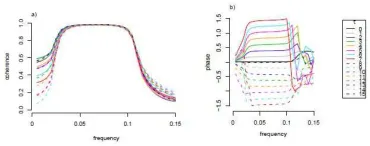
Coherence and phase analysis comparison with Fourier-based methods. For comparison
with established Fourier-based techniques, we also performed coherence analysis of stationary,
regularly sampled vector autoregressive (VAR) processes, as well as phase analysis of the signals
described above. For regularly sampled stationary processes, we compared our estimates to the
well-behaved Fourier estimates, while in the presence of sampling irregularity/nonstationarity, we
compared our method to the short-time Fourier transform (STFT) and the Lomb-Scargle method.
For brevity, we do not include the coherence and phase comparison plots here, but they can be
found in Appendix A of the supplementary material.
Specifically, in the supplementary material we illustrate the coherence estimates obtained through
both a classical Fourier-based approach and our lifting-based method on two bivariate VAR
pro-cesses. The resulting estimates agree very well, with the lifting-based estimate displaying a slight
depreciation when compared to the well-behaved Fourier estimates, suited for regular sampling
and stationary process behaviour. However, in general if the data is believed to be amenable to
be analysed with standard methodology, Fourier-based estimation should be preferred to the
pro-posed method which was specifically designed to offer a solution for the challenging situations that
include irregular sampling.
As already highlighted, traditional methods do not readily handle data that feature both
po-tential nonstationarities and irregular sampling, thus STFT required further intervention while the
Lomb-Scargle method failed to account for nonstationarity. Thus in order to obtain the desired
phase analysis, we mapped the irregular data to a regular grid (by e.g. interpolation) and then used
STFT in order to capture the nonstationary time-frequency content of the data. The Lomb-Scargle
analysis naturally dealt with the sampling irregularity, but assumed stationarity and therefore it did
little resolution in time or frequency, possibly due to the spectral blurring induced by the
over-lapping windows in the STFT as noted in Shumway and Stoffer (2013). Furthermore, for signals
sampled over different irregular grids, the method creates additional blurring in the phase plot. By
contrast, the Lomb-Scargle method is able to deal naturally with the irregular sampling structure
of the signals, but it does not contain any time-phase information. In addition, there is no marked
distinction in frequency where the phase is large, unlike for that of our complex lifting method (see
Figure 5). These features yet again highlight the appeal of our technique.
3.3.2 Simulated data with varying time delay
The next example explores the effect of increasing the time delay between two signals. For each
value ofτ=1, . . . ,15, the series{(xk, fk1, fk2)}200k=1are simulated following
fk1 = sin 2πxk 30
!
+ζk1,
fk2 = sin 2π(xk−τ) 30
!
+ζk2,
where (xk+1 − xk) ∈ {n/10 : n = 10,11, . . . ,30} and (n1−1)Pnk−=11(xk+1 − xk) = 2, ζk1 and ζk2 are
independent, identically distributed Gaussian variables with mean zero, variance 0.22.
Just as in the classical (Fourier) analysis, it is interesting to inspect the coherence and phase
across frequencies (here, scales) in order to relate the common behaviour of the two series and
pos-sible time delays, respectively. The estimated coherence and phase corresponding to the increasing
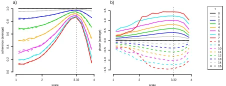
τ = 1, . . . ,15 are shown in Figure 7. To give an overall sense of the coherence and phase
magni-tude over time, the estimates are averaged over the full time range to giveρ(ℓi)= 2001 P200
k=1ρxk(ℓ
i).
We used P=750 randomly sampled trajectories and discretised using J∗= 20 artificial scales.
When τ = 0, the coherence is 1 and the phase is 0. For τ , 0 the coherence is greatest at a
scale of log2(30/3), corresponding to the period of variation (T = 30) in the data. The coherence
intensity and response over scale are affected by the magnitude of the time delay. The coherence
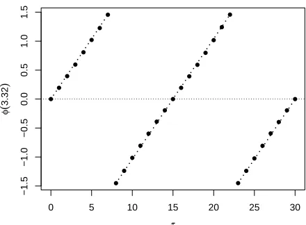
is lowest at time delays around 7.5 (T/4), and at these shifts the peak at scale log2(30/3) is also
more pronounced. Atτ=15 (T/2) the signals are sign reversed versions of each other and, again,
response varies as a function of time delay and alternates between positive and negative values,
with|φ(ℓi)|maximised atℓi = T/4. This is displayed in Figure 8 which shows the estimated phase
at scale log2(30/3) as a function of time delay.
For completeness, we also provide a direct comparison with classical Fourier coherence and
phase estimation when the signals are regularly sampled (see Figure 9). Whilst the overall
be-haviour is similar for both the classical andCNLT methods, the Fourier method displays less
vari-ability across coherence estimates with the changing time delay (Figure 9, left), as well as more
localised phase-frequency information (Figure 9, right). However, in general, note that if the data
is believed to be amenable to be analysed with standard methodology, this should be preferred to
the proposedCNLT method which was specifically designed to offer a solution for the challenging
situations that include irregular sampling.
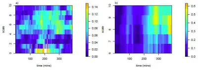
3.3.3 Financial time series
In this section we demonstrate the use of the proposed complex-valued lifting transform through an
application to financial data consisting of prices of all trades on 1 March 2011 (in normal trading
hours) for two IT companies, Baidu and Google, both traded on the NASDAQ stock exchange.
Comparison of the two companies is of interest as the main product of both is a search engine, but
they are based in different geographical regions.
Often several trades per second occur and in this case the last quoted value for each second is
selected. Thus the finest sampling interval is one second, but as there are seconds with no trades,
the time series are not equally spaced. For the analysis we consider the returns of each series– for
Google, the series contains 7984 observations with an average sampling distance of 2.93 seconds
and range 1 to 48; for Baidu, the series contains 6535 observations with an average sampling gap
of 3.58 seconds and range 1 to 52.
The data was analysed using the methodology described in Section 3.2 using J∗= 15 artificial
scales and T∗ = 390 artificial time intervals (each time interval has a width of 60 seconds). The
estimates were smoothed over time using a window width of M1 = 60 minutes at the finest scale
and increasing by a factor of 1.05, to provide a larger smoothing window for each subsequent
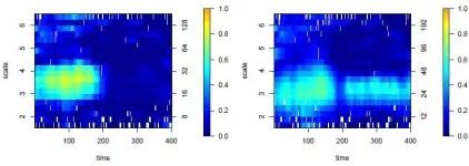
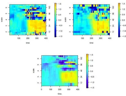
resulting coherence estimate is an increased coherence around scale 6, corresponding to a Fourier
frequency of T ≈ 3 minutes. The magnitude of the coherence at this scale is seen to be more
pronounced towards the end of the day. There is also a period of higher coherence observed in the
middle of the day, at low wavelet scales (corresponding to high frequency information).
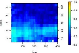
One usual treatment of such irregular data would be to consider it in terms of the one minute
average returns. The estimated coherence using the aggregated data is shown in Figure 10b),
where J∗ =10 artificial scales and T∗= 78 artificial time intervals (each representing a range of 5
minutes) were used. Notice that finer behaviour details are erased, reflecting the coarser sampling
rate of the averaged data, and that spurious coherence is unsurprisingly induced by aggregation.
4
Real nonparametric regression using complex lifting
As with the traditional wavelet and lifting transforms, our proposed complex nondecimated lifting
transform can be used for nonparametric regression problems, including those with nonequispaced
sampling design. In a nutshell, the proposed smoothing procedure can be described as (i) perform
the complex lifting transform of the original data, (ii) combine the real and imaginary coefficients
into a statistic to undergo thresholding/shrinkage and (iii) take the inverse lifting transform to
obtain the estimated unknown signal. A detailed description and estimator properties are provided
in Appendix B (supplementary material).
We briefly illustrate the application of this technique to the ethanol data example from Brinkman
(1981) that has been analyzed extensively, see for instance Kovac and Silverman (2000) and
Cleve-land et al. (1992). The data consist of 88 measurements of NOx exhaust emissions from an
automo-bile test engine, together with corresponding engine equivalence ratios, a measure of the richness
of the air/ethanol mix (Kovac and Silverman, 2000; Loader, 1999). Because of the nature of the
experiment, the observations are not available at equally-spaced design points, and the variability
is larger for low equivalence ratios.
We estimate the ratio-dependent (heteroscedastic) variance using a wavelet domain local
esti-mation procedure similar to that of Kovac and Silverman (2000) and Nunes et al. (2006).
both identify changes in slope around 0.7 and 0.9. However, the magnitude and duration of these
effects appear to be different between the two estimates. The real-valued adaptive lifting estimate
has an overall similar appearance albeit being less smooth and featuring more abrupt changes that
are unlikely to be true features of the process. In this example, the true shape of the ethanol curve
is of course unknown, however we believe that it is more likely to be smooth. Hence it is pleasing
to see that even visually our estimator does a good job in this case.
Acknowledgements
The authors would like to thank the two anonymous referees for helpful suggestions which led
to a much improved manuscript. Piotr Fryzlewicz’s work was supported by the Engineering and
References
Abbas, A. and Tran, T. D. (2006). Multiplierless design of biorthogonal dual-tree complex wavelet
transform using lifting scheme. In IEEE International Conference on Image Processing. 2006,
pages 1605–1608. IEEE.
Abramovich, F., Bailey, T., and Sapatinas, T. (2000). Wavelet analysis and its statistical
applica-tions. Journal of the Royal Statistical Society D, 49(1):1–29.
Allen, J. (1977). Short-term spectral analysis, and modification by discrete fourier transform. IEEE
Transactions on Acoustics Speech and Signal Processing, 25(3):235–238.
Barber, S. and Nason, G. P. (2004). Real nonparametric regression using complex wavelets.
Jour-nal of the Royal Statistical Society B, 66(4):927–939.
Bos, R., de Waele, S., and Broersen, P. M. T. (2002). Autoregressive spectral estimation by
ap-plication of the Burg algorithm to irregularly sampled data. IEEE Transactions on Instrumental
Measurement, 51(6):1289–1294.
Brinkman, N. D. (1981). Ethanol fuel-a single-cylinder engine study of efficiency and exhaust
emissions. Technical report, SAE Technical Paper.
Broerson, P. M. T. (2008). Time series models for spectral analysis of irregular data far beyond the
mean data rate. Measurement Science and Technology, 19:1–13.
Cleveland, W., Grosse, E., and Shyu, W. (1992). Local regression models. In Statistical Models in
S. Chambers, J.M. and Hastie, T.J. (eds).
Engle, R. F. (2000). The econometrics of ultra-high-frequency data. Econometrica, 68(1):1–22.
Erdogan, E., Ma, S., Beygelzimer, A., and Rish, I. (2004). Statistical models for unequally spaced
time series. In Proceedings of the 5th SIAM International Conference on Data Mining. SIAM.
Fernandes, F. C. A., Selesnick, I. W., van Spaendonck, R. L. C., and Burrus, C. S. (2003). Complex
Foster, G. (1996). Wavelets for period analysis of unevenly sampled time series. The Astronomical
Journal, 112(4):1709–1729.
Frick, P., Grossman, A., and Tchamitchian, P. (1998). Wavelet analysis for signals with gaps.
Journal of Mathematical Physics, 39:4091–4107.
Genc¸ay, R., Dacorogna, M., Muller, U. A., Pictet, O., and Olsen, R. (2001). An Introduction to
High-Frequency Finance. Academic press.
Hall, P. and Patil, P. (1996). On the choice of smoothing parameter, threshold and truncation
in nonparametric regression by non-linear wavelet methods. Journal of the Royal Statistical
Society B, pages 361–377.
Jacobsen, E. and Lyons, R. (2003). The sliding DFT. IEEE Signal Processing Magazine, 20(2):74–
80.
Jansen, M., Nason, G., and Silverman, B. (2001). Scattered data smoothing by empirical bayesian
shrinkage of second generation wavelet coefficients. In Unser, M. and Aldroubi, A., editors,
Wavelet Applications in Signal and Image Processing IX, volume 4478, pages 87–97. SPIE.
Jansen, M., Nason, G. P., and Silverman, B. W. (2009). Multiscale methods for data on graphs
and irregular multidimensional situations. Journal Of The Royal Statistical Society Series B,
71(1):97–125.
Jansen, M. H. and Oonincx, P. J. (2005). Second Generation Wavelets and Applications. Springer
Science & Business Media.
Kingsbury, N. (1999). Image processing with complex wavelets. Philosophical
Transac-tions of the Royal Society of London A: Mathematical, Physical and Engineering Sciences,
357(1760):2543–2560.
Kingsbury, N. (2001). Complex wavelets for shift invariant analysis and filtering of signals.
Knight, M. I. and Nason, G. P. (2009). A ‘nondecimated’ lifting transform. Statistics and
Com-puting, 19:1–16.
Knight, M. I. and Nunes, M. A. (2012). nlt: a nondecimated lifting scheme algorithm. R package
version 2.1-3.
Knight, M. I., Nunes, M. A., and Nason, G. P. (2012). Spectral estimation for locally stationary
time series with missing observations. Statistics and Computing, 22(4):877–895.
Kovac, A. and Silverman, B. W. (2000). Extending the scope of wavelet regression
meth-ods by coefficient-dependent thresholding. Journal of the American Statistical Association,
95(449):172–183.
Lina, J.-M. and Mayrand, M. (1995). Complex Daubechies wavelets. Applied and Computational
Harmonic Analysis, 2(3):219–229.
Loader, C. (1999). Local Regression and Likelihood. Springer: New York.
Lomb, N. (1976). Least-squares frequency analysis of unequally spaced data. Astrophysics and
Space Science, 39(2):447–462.
L¨utkepohl, H. (2005). New introduction to multiple time series analysis. Springer Science &
Business Media.
Magarey, J. and Kingsbury, N. (1998). Motion estimation using a complex-valued wavelet
trans-form. IEEE Transactions on Signal Processing, 46(4):1069–1084.
Nason, G. and Silverman, B. (1995). The stationary wavelet transform and some applications. In
Antoniadis, A. and Oppeheim, G., editors, Wavelets and Statistics, volume 103 of Lecture Notes
in Statistics, pages 281–300. New York: Springer-Verlag.
Nason, G. P. (2008). Wavelet Methods in Statistics with R. Springer.
Nason, G. P., von Sachs, R., and Kroisandt, G. (2000). Wavelet processes and adaptive estimation
Nunes, M. A. and Knight, M. I. (2012). adlift: an adaptive lifting scheme algorithm.
Nunes, M. A., Knight, M. I., and Nason, G. P. (2006). Adaptive lifting for nonparametric
regres-sion. Statistics and Computing, 16(2):143–159.
Ombao, H., Raz, J., von Sachs, R., and Guo, W. (2002). The SLEX model of a non-stationary
random process. Annals of the Institute of Statistical Mathematics, 54(1):171–200.
Park, T., Eckley, I. A., and Ombao, H. C. (2014). Estimating time-evolving partial coherence
between signals via multivariate locally stationary wavelet processes. IEEE Transactions on
Signal Processing, 62:5240–5250.
Percival, D. B. and Walden, A. T. (2006). Wavelet Methods for Time Series Analysis, volume 4.
Cambridge University Press.
Portilla, J. and Simoncelli, E. P. (2000). A parametric texture model based on joint statistics of
complex wavelet coefficients. International Journal of Computer Vision, 40(1):49–70.
Priestley, M. B. (1983). Spectral Analysis and Time Series. Volumes I and II in 1 book. Academic
Press.
R Core Team (2013). R: A Language and Environment for Statistical Computing. R Foundation
for Statistical Computing, Vienna, Austria.
Rehfeld, K., Marwan, N., Heitzig, J., and Kurths, J. (2011). Comparison of correlation analysis
techniques for irregularly sampled time series. Nonlinear Processes in Geophysics, 18(3):389–
404.
Reinsel, G. C. (2003). Elements of multivariate time series analysis. Springer Science & Business
Media.
Sanderson, J. (2010). Wavelet methods for time series with bivariate observations and irregular
sampling grids. PhD thesis, University of Bristol, UK. https://www.shef.ac.uk/scharr/
Sanderson, J., Fryzlewicz, P., and Jones, M. W. (2010). Estimating linear dependence between
nonstationary time series using the locally stationary wavelet model. Biometrika, 97(2):435–
446.
Scargle, J. (1982). Studies in astronomical time series analysis. II- Statistical aspects of spectral
analysis of unevenly spaced data. The Astrophysical Journal, 263:835–853.
Schr¨oder, P. and Sweldens, W. (1996). Building your own wavelets at home. ACM SIGGRAPH
course notes.
Selesnick, I., Baraniuk, R., and Kingsbury, N. (2005). The dual-tree complex wavelet transform.
IEEE Signal Processing Magazine, 22(6):123–151.
Shui, P.-L., Bao, Z., and Tang, Y. Y. (2003). Three-band biorthogonal interpolating complex
wavelets with stopband suppression via lifting scheme. IEEE Transactions on Signal Processing,
51(5):1293–1305.
Shumway, R. H. and Stoffer, D. S. (2013). Time Series Analysis and its Applications. Springer
Science & Business Media.
Sweldens, W. (1996). The lifting scheme: A custom-design construction of biorthogonal wavelets.
Applied and Computational Harmonic Analysis, 3(2):186–200.
Van´ıˇcek, P. (1971). Further development and properties of the spectral analysis by least-squares.
Astrophysics and Space Science, 12(1):10–33.
Witt, A. and Schumann, A. Y. (2005). Holocene climate variability on millennial scales recorded
in greenland ice cores. Nonlinear Processes in Geophysics, 12(3):345–352.
Wolff, E. W. (2005). Understanding the past-climate history from Antarctica. Antarctic Science,
>
...
>
>
>
>
[image:28.612.194.419.87.312.2]>
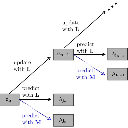
Figure 1: The complex-valued lifting scheme (C-LOCAAT). Solid lines correspond to the steps
of the standard LOCAAT lifting scheme whereas dotted lines indicate the extra prediction step
required for the complex-valued scheme. After (n−R) applications, the function can be represented
as a set of R smooth coefficients{cr−1,i}i∈Sn−R and (n−R) detail coefficients{λjk +iμjk}k∈Dn−R, each
time
scale
d1
time
scale
d2
time
scale
x1x2x3x4 x5 x6
time
scale
I1, 2
l1
l2
[image:29.612.197.419.90.137.2]x1x2x3x4 x5 x6
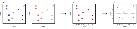
Figure 2: Construction of bivariateCNLT transform for time series observed on the same sampling
grid (x refers to time here): a) univariateCNLT is applied using the same set of trajectories for both
series and yields two sets of detail coefficients{dx1,kp}p,kand{d
2,p
xk }p,k; b) theCNLT transform consists
of combinations of coefficients from each series; c) the detail coefficients are averaged within each
time
scale
a)
d1
time
scale
d2
time
scale
b)
D1
time
scale
D2
time
scale
c)
I1, 2
l1
l2
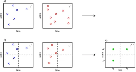
[image:30.612.200.419.94.210.2]t1 t2
Figure 3: Construction of bivariateCNLT transform for time series observed on different sampling
grids (x refers to time here): a) each series is lifted individually as described in Section 2.3; b)
the sets of coefficients in each grid square. The coefficients are sampled so that there is the same
number in the grid square of each series; c) the coefficients of each series are combined to form
Figure 5: Phase estimation using the complex-valued lifting scheme: data observed on the same
irregular sampling grid (left); data observed on different irregular sampling grids (right); data
scale coherence (a v er age) 0.0 0.2 0.4 0.6 0.8 1.0
1 2 3.32 4
a) scale phase (a v er age) −1.5 −1.0 −0.5 0.0 0.5 1.0 1.5
1 2 3.32 4
b) τ 0 1 2 3 4 5 6 7 8 9 10 11 12 13 14 15
Figure 7: a) Coherence and b) Phase between f1and f2 (Section 3.3.2) as a function of scale and
τ∈0,15. Forτ, 0 the coherence and (absolute) phase are greatest at scale log
[image:34.612.192.418.89.175.2]0 5 10 15 20 25 30
−1.5
−1.0
−0.5
0.0
0.5
1.0
1.5
τ
φ
(
3.32
[image:35.612.196.416.105.267.2])
Figure 8: Estimated phase between f1 and f2 (Section 3.3.2) at scale log2(30/3) (equivalent to a
Figure 9: a) Coherence and b) Phase between f1 and f2(Section 3.3.2) as a function of frequency
[image:36.612.207.392.103.176.2]Figure 10: Coherence between Google and Baidu using methods from Section 3.2: a) computed
on different irregular sampling grids; b) computed using one minute averages. Scale gets coarser
Figure 11: Ethanol data and estimates. Small circles=data; solid line=estimate. Top-left: smooth-ing spline with cross-validated smoothsmooth-ing parameter; top-right: multiple observation adaptive
lift-ing uslift-ing R-lift with heteroscedastic variance computation and EbayesThresh posterior median
thresholding; bottom: C-AP1S with heteroscedastic variance computation and level-dependent