A branch-and-price approach for solving the train unit scheduling problem

This is a repository copy of

A branch-and-price approach for solving the train unit

scheduling problem

.

White Rose Research Online URL for this paper:

http://eprints.whiterose.ac.uk/105182/

Version: Accepted Version

Article:

Lin, Z and Kwan, RSK (2016) A branch-and-price approach for solving the train unit

scheduling problem. Transportation Research Part B: Methodological, 94. pp. 97-120.

ISSN 0191-2615

https://doi.org/10.1016/j.trb.2016.09.007

© 2016 Elsevier Ltd. All rights reserved. This manuscript version is made available under

the CC-BY-NC-ND 4.0 license http://creativecommons.org/licenses/by-nc-nd/4.0/.

[email protected] https://eprints.whiterose.ac.uk/ Reuse

Unless indicated otherwise, fulltext items are protected by copyright with all rights reserved. The copyright exception in section 29 of the Copyright, Designs and Patents Act 1988 allows the making of a single copy solely for the purpose of non-commercial research or private study within the limits of fair dealing. The publisher or other rights-holder may allow further reproduction and re-use of this version - refer to the White Rose Research Online record for this item. Where records identify the publisher as the copyright holder, users can verify any specific terms of use on the publisher’s website.

Takedown

If you consider content in White Rose Research Online to be in breach of UK law, please notify us by

A branch-and-price approach for solving the train unit

scheduling problem

Zhiyuan Lin∗1and Raymond S. K. Kwan†1

1_{School of Computing, University of Leeds, Leeds, LS2 9JT, United Kingdom}

September 15, 2016

Abstract

We propose a branch-and-price approach for solving the integer multicommodity flow model for the network-level train unit scheduling problem (TUSP). Given a train operator’s fixed timetable and a fleet of train units of different types, the TUSP aims at determining an assignment plan such that each train trip in the timetable is appropriately covered by a single or coupled train units. The TUSP is challenging due to its complex nature. Our branch-and-price approach includes a branching system with multiple branching rules for satisfying real-world requirements that are difficult to realize by linear constraints, such as unit type coupling compatibility relations and locations banned for coupling/decoupling. The approach also benefits from an adaptive node se-lection method, a column inheritance strategy and a feature of estimated upper bounds with node reservation functions. The branch-and-price solver designed for TUSP is capable of handling instances of up to about 500 train trips. Computational experiments were conducted based on real-world problem instances from First ScotRail. The results are satisfied by rail practitioners and are generally competitive or better than the manual ones.

Keywords:Rolling stock scheduling; Train unit scheduling; Integer multicommodity flow prob-lems; Branch-and-price

1

Introduction

1.1 Train unit scheduling problem

Atrain unit is a self-propelled non-splittable fixed set of train cars(carriages), which is the most commonly used passenger rolling stock in the UK and many other European countries. A train unit is able to move in both directions on its own. Train units are classified into types having different characteristics. A train unit can be coupled with other units of the same or compatible types.

Given a rail operator’s timetable on one operational day, a fleet of train units of different types and a rail network of routes, stations and infrastructures, thetrain unit scheduling problem(TUSP) (Lin and Kwan, 2014) refers to the planning of how timetabled trains are covered by a single or coupled train units from the fleet. From the perspective of a train unit, scheduling assigns a sequence of trains to it as its daily workload. A route refers to a unique path in a rail network between two locations. The

∗_{[email protected] (Corresponding author)}

TUSP may also include auxiliary activities, e.g. empty-running insertion, coupling/decoupling con-trol, platform assignment, platform/siding/depot capacity concon-trol, re-platforming, reverse, shunting movements from/to sidings or depots and unit blockage resolution. Capacity control is needed when there are several train units staying at the same berthing place such as a platform/siding/depot and it is to make sure the capacity of the berthing place is not exceeded. Re-platforming refers to the opera-tion to shunt a train unit from its arrival platform to a different departure platform. Reverse activities usually occur at a dead-end platform such that the train unit will depart in the opposite direction to its arrival. A reverse activity will change the unit permutation if a train is formed by coupled units, where the unit permutation refers to the order of units (e.g. front, middle, rear) in a coupled forma-tion. More details on the train unit operation rules can be found in Lin and Kwan (2014). In some cases, maintenance and unit overnight balance planning (or unit cycles) are also included; however in the UK, they are often achieved at later stages after train unit scheduling. A similar problem in the literature to the TUSP is thetrain unit assignment problem(TUAP) (Cacchiani et al., 2010b, 2012b, 2013b). Another relevant problem isrolling stock circulation problem(Schrijver, 1993; Alfieri et al., 2006; Peeters and Kroon, 2008), which however has different problem definitions than TUAP and TUSP.

1.2 A branch-and-price solver for TUSP

This paper addresses the particular issue of designing an efficient branch-and-price ILP solver for the integer multicommodity flow (IMCF) models used for the network-level TUSP. An IMCF model is proposed in Cacchiani et al. (2010b) for the TUAP, where the integer program is solved by an LP-based diving heuristic. A two-phase approach is presented in Lin and Kwan (2014) for the TUSP. The first phase is a fixed-charge IMCF model, where for most tested real-world instances the integer solver only generated columns at the root node in the BB tree, such that the solution qualities are not guaranteed to be exact. Although exact methods are used for the rolling stock circulation problems, the problem definitions are different from Cacchiani et al. (2010b) or Lin and Kwan (2014). For the TUAP/TUSP, there is no exact solution method in literature that is able to handle realistic problem sizes especially in the UK as far as the authors are aware.

A branch-and-price solver proposed in Lin and Kwan (2014) mainly uses columns from root node in the BB tree in most tested instances because of its limited capability. No customized branching or node selection strategy is used in the solver. No method is used to strengthen the weak LP-relaxation. The node-family variables are also not capable in handling all possible combination-specific coupling upper bound requirements. Compared with the aforementioned solver, significant improvements have been made in the proposed branch-and-price approach. It is capable of handling real-world instances of up to around 500 trains. The improvements include: (i) A branching system with multiple branching rules including two customized rules as train-family branching and banned location branching; (ii) An adaptive node selection method; (iii) A column inheritance strategy; (iv) A branch-and-bound (BB) system with estimated upper bounds and tree node reservation, and (v) the use of convex hulls for satisfying difficult real-life constraints.

1.3 Contributions

The main contribution of this paper is the design of a customized branch-and-price solver for solving the TUSP. While the TUAP studied by Cacchiani et al shares similar features of TUSP, the solution approaches for the TUAP are all based on heuristics. For instance, in Cacchiani et al. (2010b), an LP based diving heuristics is used for solving the integer multicommodity flow ILP model. In Cacchi-ani et al. (2013b), a fast heuristics is applied in conjunction with Lagrangian relaxation. Moreover, compared with the TUAP, additional real-life requirements that are crucial in UK railway opera-tions are considered in the TUSP, such as train unit type compatibility relaopera-tions, locaopera-tions banned for coupling/decoupling and combination-specific coupling upper bounds. Customized strategies to ac-commodate those requirements have been implemented in the branch-and-price solver, such as local convex hulls, branching on train families and banned locations. Finally, some advanced techniques are used in the solver for speeding up the solution process, such as an adaptive node selection method combined with best-first and depth-first, column inheritance and estimated upper bound. Computa-tional experiments have proved their usefulness for the tested real-world instances.

It is worth mentioning that some constraints considered in Cacchiani et al. (2010b), such as main-tenance and overnight balance, are not included in our solver. This is because they are conventionally regarded as separate stages in the UK railway industry. Moreover, in Cacchiani et al. (2010b) and Cacchiani et al. (2013b), larger numbers of different unit types (up to 10 for real-world instances and 20 for realistic instances) are experimented. In our work, up to three different types are experimented, which is based on the real-world operational rules of the operator’s network.

1.4 Organization of the paper

The remainder of this paper is organized as follows. Section 2 surveys the relevant literature. Sec-tion 3 describes the TUSP in more details. SecSec-tion 4 presents the model and integer linear program-ming formulation. Section 5 gives the branch-and-price approach for solving the above formulation. Section 6 reports computational experiments based on real-world instances. Finally we conclude this paper in Section 7.

2

Literature review

rescheduling in Cacchiani et al. (2014). For surveys on methodological approaches in general railway planning, see Caprara et al. (2007, 2011); Huisman et al. (2005).

2.1 Train unit resource planning

Train unit scheduling is a kind of rolling stock scheduling. Below, we review the researches that are directly pertinent to this field.

2.1.1 The train unit circulation problem

Although sharing a common feature as being a practice to assign train units to a given timetable, problem definitions for the train unit circulation problem are different from the TUAP and TUSP. For a train/trip at Nederlandse Spoorwegen Reizigers (NSR)1, its unique predecessor and successor are given in advance. By predecessor and successor, at least one unit should be operated according to the preset connection between the two relevant trains or trips. Often this pre-sequencing is done locally at each station based on a first-in-first-out (FIFO) basis (Fioole et al., 2006; Maróti, 2006); the fact that trains in timetables are generally well-patterned (departure and arrival times are regulated every hour or periodically) at NSR also makes the FIFO pre-sequencing practically workable. Moreover, at least one unit should follow the complete journey of its associated NSR-train. This is referred to as the “continuity requirement” (Fioole et al., 2006; Maróti, 2006). In the TUAP/TUSP, the connection possibilities among trains are left flexible such that no prescribed connection is imposed. The unit permutation (order) issue is also considered in the research on NSR. In the UK, the train timetables are not regular enough for pre-sequencing, and FIFO is thus not suitable for connecting most trains. In addition, circulation and rostering of train units are often left as a separate process in the UK railway industry.

Schrijver (1993) proposes an integer multicommodity flow model for the train unit circulation problem for a single line on a single day with two compatible unit types for NSR. In the model the nodes represent the arrival and departure events at stations and the arcs represent the trips. Flows of different commodities stand for train units of different types. The framework of this model (flow graph or time-space graph) has been used in most subsequent research on rolling stock circulation by NSR. The objective is to minimize the fleet size. As there are at most two compatible types of unit, the weak passenger demand satisfaction and coupling upper bound knapsack constraints are replaced by explicitly finding their relevant convex hulls inR2. Some local issues like time allowances and permutation restrictions regarding coupling/decoupling are ignored.

Alfieri et al. (2006) consider a problem scenario similar to Schrijver (1993). The same flow graph framework is used. The objective is to minimize the combination of fixed and variable costs of train units. Two models have been proposed. The first one ignores the unit permutation issue and satisfies the passenger demands and coupling upper bounds directly by constraints in conjunction with similar convex hull strengthening as in Schrijver (1993). The second model can handle the unit permutation issue by introducing a transition graph concept and new decision variables representing unit compositions per trip. These new composition variables also have included the conditions to comply with passenger demands and coupling upper bounds implicitly. Issues like cycles, shunting conflicts and maintenance are left to other planning stages. Also a pre-processing approach to reduce the sizes of the transition graphs is developed. The model has been applied to the line 3000 of NSR with 12 NSR-trains.

1_{A “train” at NSR does not have the same meaning as a “train” in the TUAP or TUSP. The unit composition within an}

Peeters and Kroon (2008) present a model for a train unit circulation problem for two lines of NSR with 15 NSR-trains (182 trips) and 12 NSR-trains (115 trips) respectively. Also based on the framework of a time-space graph, the model uses the aforementioned transition graph where unit compositions at each connection between the trips are explicitly enumerated and the composition transition possibilities are represented by associated decision variables. Moreover, variables and con-straints for describing unit inventories at stations are used. Dantzig-Wolfe decomposition is used for solving the model, where since the order of the joint flows are considered, the master problem is decomposed with respect to NSR-trains. Branch-and-price is applied to get integer solutions. This approach is able to handle real-world instances of NSR in a short time after fine-tuning in the branch-and-price solver.

The models in Alfieri et al. (2006) and Peeters and Kroon (2008) have employed the idea of transition graph that strongly uses the fact that all NSR-trains are running on lines such that the predecessor and successor of a train or trip are unique. Sometimes, an NSR-train will be associated with a route with a topology other than a “line”, but of a “Y” or an “X” shape, indicating that a train/trip can have two predecessors and/or two successors and thus relevant coupling/decoupling operations have to be imposed. This is called combining/splitting of a train and has been catered for in a customized way by a model proposed in Fioole et al. (2006). Real-world problems in the Noord-Oost lines with 665 trips have been tested and several fine-tuning methods are used to speed up the solution process. Near-optimal solutions for the tested instances can be found in 1900–6400 seconds.

2.1.2 The train unit assignment problem and train unit scheduling problem

The train unit assignment problem (TUAP) shares similar definitions and settings with the TUSP, especially in the sense that no trains are pre-sequenced in advance and no coupling/decoupling is allowed en route. Cacchiani et al. (2010b) present an integer multicommodity flow model for the TUAP. For each train, there is a passenger demand in the number of seats and a coupling upper bound of two units. The model can also include additional constraints for maintenance and overnight bal-ance. The model is based on a directed acyclic graph (DAG) where the nodes represent trains and the arcs represent connection possibilities. Each commodity stands for a unit type and its flow amount at a node gives the number of units of that type used there. A similar DAG framework is also used in this work and in Lin and Kwan (2014). The path formulation is reported to be more efficient in solving the TUAP. Taking advantage that no more than two units can be coupled, the LP-relaxation is strength-ened by replacing relevant knapsack constraints by their dominants (see Cacchiani et al. (2013a)). An LP-based heuristic is designed for finding the integer solutions without using a branch-and-bound tree. This heuristic is reported to be crucial in finding feasible solutions in many of the tested instances. The above model and the heuristic method has been applied to real-world instances of a regional train operator in Italy, with fleets of up to 10 distinct unit types and timetables of 528–660 trains. The heuristic is able to find solutions 10–20% better than the manual solutions in practice. Experimented on a PC with Pentium 4, 3.2GHz, 2GB RAM, and an LP-solver of ILOG-CPLEX 9.0, the solution time ranges from 1878–1932 seconds without the additional maintenance and overnight balance con-straints, and 5897–14105 seconds with those constraints. Compared with TUSP, TUAP does not consider locations banned for coupling/decoupling, unit type compatibility relations or combination-specific coupling upper bound. The objective function in the reported experiments is set to only minimize the number of used units, while in TUSP, mileage, number of empty-movements and other preferences are also included in the objective.

solution in a very short time such that it can be embedded into real-time operations in conjunction with other planing activities like timetabling. Computational experiments have been conducted for the same instances as in Cacchiani et al. (2010b) and for some larger instances of up to around 1000 trains. Comparisons with the method given in Cacchiani et al. (2010b) have been made. The same authors have proposed another fast heuristic for the same train unit assignment problem in Cacchiani et al. (2012b). The lower bound is given by solving an ILP that only considers a subset of “simultaneous” peak time trains where any two of them cannot be covered by the same unit. Real-world instances were tested and comparisons with the approaches in Cacchiani et al. (2010b, 2013b) were made. See Cacchiani (2007, 2009); Cacchiani et al. (2012a) for more of the research on the TUAP.

The train unit scheduling problem (TUSP) described in Lin and Kwan (2014) is similar to the TUAP (Cacchiani et al., 2010b), except that additional real-world requirements are considered, such as unit type coupling compatibility, locations banned for coupling/decoupling, combination-specific coupling upper bounds, and station-level unit blockage issues. A two-phase approach is presented since including station-level details into the main model would give an intractable huge-sized prob-lem. This two-level decomposition framework is justified from railway operation practice and station-based simulations. In the reported experiments, the integer solver only generated columns at the root node of the BB trees for most of the tested instances such that the exactness of the solutions cannot be guaranteed. Moreover, the integer solver reported did not use customized branching strategies and the node selection method was fixed to best-first. No attempt was made at strengthening the lower bound given by LP-relaxation. The train-family variable method for ensuring coupling compatibility and specific upper bounds also had limitations such that not all possible combination-specific upper bound scenarios can be handled.

While rolling stock scheduling usually assume unique and well-defined train capacity require-ments, in practice rail operators may consider different levels of capacity provisions. In Lin et al. (2016), the problem of train unit scheduling with bi-level capacity requirements is studied and an integer multicommodity flow model is proposed based on previous research.

2.1.3 Other research in train unit planning

Jiang et al. (2014) propose a model for scheduling additional train unit services in a double parallel rail transit line such that timetable scheduling and train unit scheduling are integrated into the model with two objectives: minimizing travel times of additional trains and minimizing shifts of initial trains. Computational experiments on real rail transit line 16 in Shanghai were tested yielding a reasonable new timetable.

Lu et al. (2016) present a solution approach for scheduling train units under the condition of their utilizations on one sector or within several interacting sectors. The method consists of two stages: a greedy stage to construct a feasible circulation plan fragment, and a stochastic disturbance to generate a whole feasible solutions or get a new feasible solution. Computational experiments on a railway corridor representing the basic feature of railway networks were reported.

2.2 Locomotive scheduling

in the UK and many other countries.

Wolfenden and Wren (1966) propose a heuristic method such that it can resize the problem scale small enough for the Hungarian algorithm to repeatedly solve updated instances until the converged optimum. This method was applied to real-world instances of British Railways and became opera-tional in May 1963, reducing the number of locomotives from 15 to 12 and giving 28% less empty-running. It is reported to be the world’s first computer-produced working schedule (Wren, 2004).

Ziarati et al. (1999) propose a model to assign locomotives to trains such that sufficient power can be used to pull the cars. It is solved by a “branch-first, cut-second” approach, where valid inequalities are inserted to strengthen the LP lower bound and to prevent the case that more than 3 types of locomotives are assigned to the same train leg. Computational experiments have been conducted for real-world instances from Canadian National Railway with 2000 trains and 26 locomotive types.

Cordeau et al. (2000, 2001a,b) present some models on the locomotive and car assignment prob-lem, employing solution methods such as Benders decomposition and heuristic branch-and-bound based on column generation. They considered a group of compatible locomotive-car combinations that travel along some part of the rail network. Later various practical constraints have been added to the model, such as the maintenance issue. Computational experiments have been performed based on the instances from VIA Rail, Canada.

Lingaya et al. (2002) study the problem of assigning cars to timetabled trains for VIA Rail, Canada. A complex model including a master plan to additional information regarding passenger de-mands is used. Coupling/decoupling activities among cars is allowed and notably the order of the cars has been explicitly considered. Some real-world requirements such as maintenance are considered as well. Dantzig-Wolfe decomposition in conjunction with a heuristic branch-and-bound procedure is employed to solve the relevant ILP. The model has been tested based on the instances from VIA Rail, Canada.

3

Problem description

We briefly list the requirements/restrictions and objectives for the TUSP. For a more detailed descrip-tion, see Lin and Kwan (2014).

3.1 Requirements and restrictions

(1) Fleet size limit: Each train operator has a fleet of units of a limited number per type. A schedule whose used unit number exceeding the fleet size limit is invalid.

(2) Type-route compatibility: There are compatibility relations among unit types and routes. As each train belongs to a route, this turns out to be a compatibility relation among unit types and trains.

(3) Time allowances: A prerequisite for two trains to be consecutively connected by the same unit is that the arrival time of the previous train should be earlier than the departure time of the next train. Extra buffering time also has to be imposed on this time gap, as well as empty-running and shunting movements if relevant.

(4) Passenger demand: Each train in the timetable should be covered by unit(s) whose total capacity satisfies a passenger demand expected for the train, which is often measured in number of seats.

(6) Unit blockage: Movements of rolling stock vehicles are strictly restricted by tracks and other rail infrastructures, which will give various blockage problems. Detecting and eliminating poten-tial blockage requires the collection of comprehensive station-level infrastructure knowledge and operation details.

(7) Coupling/decoupling: Coupling/decoupling activities are often essential for satisfying high pas-senger demands at peak time by providing more capacities. They can also be used as a way to redistribute unit resources across the network, i.e. to provide unit capacities to some trains later elsewhere rather than for the current train whose passenger demand requirement may be actually very low.

(8) Type-type compatibility: Train units of the same type are permitted to be coupled and some dif-ferent types are also allowed to be coupled. This relation is referred to as type-type compatibility. Thetrain unit familyis defined such that coupling compatible unit types belong to the same fam-ily. So far in all the problem instances in ScotRail and Southern Railway, train unit families partition the fleet into mutually exclusive subsets. Table 1 shows the unit type and family infor-mation of Southern Railway and ScotRail. The unit types are rewritten as “Type in paper” to be referred to in this paper for convenience. Note that this requirement will increase the difficulty of the problem as it is proved in Lin and Kwan (2016a) that the multicommodity flow problem with incompatible commodities is NP-hard even when the flows are allowed to be fractional (A general fractional multicommodity flow problem can be solved in polynomial time (Ahuja et al., 1993).)

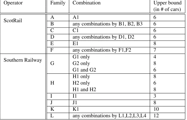
(9) Complex coupling upper bounds: When train units are coupled into a unit block, the total number of cars is restricted by an upper bound. This upper bound is often combination-specific that it is difficult to describe the relevant rules in a unified form such as linear constraints. Table 2 gives the coupling upper bound as a result of different unit combinations.

Table 1: Train unit types and their associated families of the fleets of ScotRail and Southern Railway (“c156” stands for “Class 156” and so on)

Operator Family Real Type Capacity # of cars Type in paper (seats)

ScotRail A c156 A1 145 2

B

c158 B1 136 2

c170 B2 189 3

c170S B3 198 3

C c314 C1 212 3

D c318 D1 219 3

c320 D2 230 3

E c334 E1 183 3

F c380/0 F1 208 3

c380/1 F2 282 4

Southern Railway G c171/7 G1 107 2 c171/8 G2 241 4

H c455/8 H1 316 4

c456/0 H2 152 2

I c313/1 I1 194 3

J c460/0 J1 366 8

K c442/1 K1 320 5

L

c377/1 L1 223 4 c377/2 L2 223 4 c377/3 L3 160 3 c377/4 L4 243 4

Table 2: Coupling upper bounds in number of cars associated with type combinations, regardless of other factors such as routes

Operator Family Combination Upper bound (in # of cars)

ScotRail A A1 6

B any combinations by B1, B2, B3 6

C C1 6

D any combinations by D1, D2 6

E E1 8

F any combinations by F1,F2 7

Southern Railway G

G1 only 4

G2 only 8

G1 and G2 6

H

H1 only 8

H2 only 6

H1 and H2 8

I I1 3

J J1 8

K K1 10

3.2 Objectives and solution qualities

(1) Fleet size: Because of the high costs associated with leasing and maintaining a train unit, min-imizing the number of used units is the most important objective, given the basic fleet limit requirement has been satisfied.

(2) Operational costs: Common operational costs include carriage-kilometer (mileage), empty-running movements, shunting movements, unnecessary coupling/decoupling, and so on. Carriage-kilometer refers to the total mileage incurred by all train units or all unit cars. It is natural to think that if one unit suffices in serving a train then it is a waste to use a coupled two-unit block. However, over-provision may be used to relocate unit resources across the network such that a smaller number of used units and/or less empty-running can be achieved. In this paper, shunting and unnecessary coupling/decoupling are processed in Phase-2 as a separate stage from the network flow model (see § 4.1).

(3) Preferences: Various preferences can be found in forming a real-world train unit schedule. For instance, one type of unit is more preferable than another over the same route. A practical sched-ule also needs plenty of long gaps during the off-peak time for unit maintenance. On the other hand, medium and long gaps may not be desirable at some evening times, which are regarded as irregular patterns.

4

Model description

4.1 Network-level and station-level

The entire train unit scheduling problem would be too huge-sized to be tractable if all detailed station-level restrictions such as unit blockage resolution are considered in a “once-for-all” process. There-fore, a two-phase strategy is proposed in Lin and Kwan (2014) to allow some of the station-level requirements to be omitted from a main network-level phase, whose aim is to globally assign train units to trains temporarily ignoring some station layout details such as unit permutation and the elim-ination of unit blockage. The results of the network-level phase (Pha1) would be a set of se-quenced train trips as the daily workload for a train unit in the fleet. For trains covered by multiple units, no unit permutation information is given and unit blockage may occur at the station level. The network-level phase can be regarded as an extended version of Cacchiani et al. (2010b) with more real-world constraints such as locations banned for coupling/decoupling, unit type coupling compati-bility, combination-specific coupling upper bounds and so on. Phase-2 will take the raw results from Phase-1 in a station-by-station manner to further complete local shunting plans, remove unit block-age and assign unit permutations for coupled trains. This paper will only consider the network-level phase. In Lin and Kwan (2014), a mixed integer matching model is proposed to solve Phase-2. In practice, it is sufficient to use a visual interactive software, e.g. TRACS-RS (Tracsis plc, 2016), to handel the basic tasks realized by the above model. The results of Phase-1 are uploaded to the soft-ware and train connections at each station will be displayed in detail. A user of the softsoft-ware thus can adjust the schedules if unit blockage exists or assign correct unit permutations for trains with coupled units.

them such as connection time allowances involving coupling/decoupling and penalizing redundant coupling/decoupling can be effectively achieved in Phase-2 by TRACS-RS. Therefore, here a standard integer multicommodity flow problem omitting the “fixed-charge” variables is considered.

4.2 A network-level framework based on DAG representation

A network-level DAG representation (Cacchiani et al. (2010b), Lin and Kwan (2014)) is summarized here for completeness. For the DAGG _{= (}N _,A_{), we define a node set}N _{=N∪ {s,t}, whereNis}

the set oftrain nodesrepresenting trains in the timetable, ands andtare thesourceandsinknode. An arc set is defined asA _{=A∪A0, whereAis theconnection-arcset andA0thesign-on/off arcset.}

A connection-arca∈Alinks two train nodes iand j (a= (i,j), i,j∈N), representing a potential connection such that after serving trainia unit can continue to serve train jas its next task. To be specific, if the time gap between two trains are greater than or equal to the minimum turnaround time, then a connection arc will be added between the two nodes; otherwise, no arc between them will be created. When extra time such as empty-running or shunting is involved, it should be also considered in validating the relevant time slacks. A sign-on arc(s,j)∈A0starts fromsand ends at a train node j∈N; a sign-off arc(j,t)∈A0starts from a train node j∈Nand ends att. Generally all train nodes

have a sign-on arc and a sign-off arc. δ−(j) andδ+(j)denote all arcs that terminate at / originate from node jrespectively. Finally, ans-tpath p∈PinG _{represents a sequenced daily workload (the}

train nodes in the path) for a unit.

For the fleet, we denoteKthe set of all unit types, corresponding to the commodities in a mul-ticommodity flow model. As for type-route compatibility, type-graphsGk _{representing routes each} typek∈K can serve are constructed based onG_{, as well as the components of}G_{, e.g.P}k _andAk refer to the set of all paths and arcs in type-graphGk _{respectively. We call an arc in a type-graph} Gk_{,k∈Katype-arc; on the other hand, we call an arc in the original graphG ablock-arc.}

4.3 Arc formulation and train convex hulls

First, an arc formulation based on the network-level framework is given as,

(AF) min

∑

k∈K

∑

caxa (1)

s. t.

∑

a∈δk

+(s)

xa≤bk0, ∀k∈K; (2)

∑

−(j)

xa−

∑

+(j)

xa=0, ∀j∈N,∀k∈K; (3)

∑

∑

−(j)

H_fj_,kxa≤hj_f, ∀f ∈Fj,∀j∈N; (4)

xa∈Z+, ∀a∈Ak,∀k∈K;. (5)

different connection possibilities. For instance, long gaps during off-peak hours as mentioned in § 3.2 will have their preference costs multiplied by a sub-weight of 0.5. Carriage-kilometers and preferences are combined into adjusted arc costs for the arcs. Constraints (2) ensure the number of deployed units for each typek∈K is within its fleet size limit bk₀. Constraints (3) are to force the flow conservation balance at each train node. Constraints (4) are the “train convex hull” constraints to be described in detail later. They are used to satisfy the passengers’ demands and the combination-specific coupling upper bounds. Finally Constraints (5) give the variable domain wherexa∈Z+,∀a∈ Ak_{,∀k∈Kindicates the flow amount (number of units) at type-arca∈A}k_.

In order to handle the complex combination-specific coupling upper bounds, which are commonly seen in the fleets of Southern Railway and ScotRail, we use a method presented in Lin and Kwan (2016b) based on the computation of “local convex hulls” per train. In the rolling stock scheduling literature, similar ideas in constructing local convex hulls can be found in Cacchiani et al. (2010b, 2013a); Schrijver (1993); Fioole et al. (2006); Alfieri et al. (2006); Ziarati et al. (1999), where local convex hulls are solely used to strengthen LP relaxation though.

LetKj be the set of permitted types for train j∈N, and wj = (w₁j,w₂j,· · ·,w_|j_Kj|)T ∈Z Kj

+ be a unit combination vector for j, wherew_kj stands for the number of units of typekused for j. Aunit combination setis defined as:

Wj:=

wj∈ZK+j

∀wj: a valid unit combination for train j

,∀j∈N, (6)

such that

(i) ∑_k∈K

jqkw

j

k≥rj, whereqk is the capacity of unit typekandrjis the passenger demand require-ment, both measured in numbers of seats.

(ii) ∑_k∈Kjvkw_kj ≤u(wj),∃wj ∈Wj being used, where vk is the number of cars for unit typek and

u(wj_{)is the coupling upper bound in number of cars allowed for combinationw}j_.

(iii) the used types (k:w_kj>0) are compatible.

For allWj in our problem instances, due to their small dimensions (e.g. |Kj| ≤4,∀j∈N in the ScotRail datasets), and numbers of points (e.g.|Wj| ≤9,∀j∈Nin the ScotRail datasets), it is possible to explicitly compute the convex hulls of all unit combination sets by some well-established convex hull computation algorithms, e.g. the QuickHull algorithm (Barber et al., 1996). For computational feasibility in computing local convex hulls for problems with higher dimensions and larger number of points, see Lin and Kwan (2016b). Such convex hulls associated with each train are referred to as

train convex hullsas

conv(Wj) =

wj∈RKj

+

Hjwj≤hj

, ∀j∈N, (7)

described by a set of nonzero facets f∈Fj inRK+j, withHj∈RFj×Kj andh∈RFj. Finally, by variable conversionw_kj=∑_a∈δk

−(j)xa, we have the following train convex hull constraints:

∑

∑

−(j)

H_fj_,kxa≤hj_f, ∀f ∈Fj,∀j∈N, (8)

whereH_fj_,kis the entry of nonzero facet f and typekinHj andhj_f is the entry of nonzero facet f in

4.4 Path formulation

LetMx≤bbe the matrix form of Constraints (2)–(3), and letH andhbe the coefficient matrix and right-hand side. Also letXk_={x∈ZAk

+ |Mkxk≤bk} andck,Mk,Hk,xkthe corresponding components with respect to typek. Assume that the coefficients inM,b,H,hare all integers. We rewrite(AF)as:

(AF′) min

∑

ckTxk (9)

s. t.

∑

k∈K

Hkxk≤h; (10)

xk∈Xk,∀k∈K. (11)

It is well-known thatMk,k∈K are totally unimodular (Cook et al., 1998). ThereforeQk ={x∈

RA+k|Mkx≤bk},∀k∈Kare integral and the corresponding decomposed subproblems can be solved efficiently. Moreover, the following Theorem 1 can be derived from Gallo and Sodini (1978) and Vohra (2011):

Theorem 1. An extreme point of Qk={x∈RA+k|Mkx≤bk},bk= (bk0,0, . . . ,0)T is either the null point0 or a feasible solution corresponding to a single path with a magnitude of bk₀. A feasible solution corresponding to a single path with a magnitude of bk₀is an extreme point of Qk.

Let{xp}_p∈Pkbe the nonzero extreme points of conv(Xk), and let ˆxp= 1

bk 0

xp. By applying Dantzig-Wolfe decomposition (Dantzig and Dantzig-Wolfe, 1960), the following “extensive” formulation based on paths can be derived, whereyprepresents the flow amount used on path p:

(PF) min

∑

∑

ckTxˆp

yp (12)

s. t.

∑

k∈K

∑

Hkxˆpyp≤h; (13)

∑

yp≤bk0, ∀k∈K; (14)

yp∈Z+, ∀p∈Pk,∀k∈K. (15)

In fact(PF)can be re-expressed into a more “intuitive” formulation that is self-explanatory based on the meaning ofyp, which reads:

(PF′) min

∑

∑

cpyp (16)

s. t.

∑

p∈Pk

yp≤bk0, ∀k∈K; (17)

∑

∑

j

H_fj_,kyp≤hj_f, ∀f ∈Fj,∀j∈N; (18)

yp∈Z+, ∀p∈Pk,∀k∈K. (19)

We leave the proof of the above equivalence between(PF)to(PF′_{)to Appendix A.}

It is worth mentioning that the lower bound given by the LP relaxation of the path formulation

(PF′) is the same as the one given the arc formulation(AF), since the decomposed partsXk,k∈K

are integral. Due to the same reason, the lower bound given by the Lagrangian relaxation on(AF)by relaxing Constraints (4) is the same as the above two bounds.

5

A branch-and-price solver

In this section, a branch-and-price solver for solving the path formulation(PF)(and (PF′)) is pre-sented, from which many of the techniques used can also be applied to the path formulations of the “fixed-charge” version in Lin and Kwan (2014), either directly or with certain modifications.

5.1 Branch-and-price and column generation

Branch-and-price (Barnhart et al., 1998) is a high-level framework for solving large-scale ILPs by combining branch-and-bound (BB) (Wolsey, 1998) and column generation (Lübbecke and Desrosiers, 2002; Desrosiers and Lübbecke, 2005). In a generic branch-and-bound framework, if only the BB tree’s root node is solved by column generation, then the root may not contain all the columns needed for finding an optimal integer solution. Thus branch-and-price calls for the need to also perform column generation not only at the root, but also at the leaf nodes of the BB tree. Branch-and-price is used in Peeters and Kroon (2008) for solving the rolling stock circulation problem.

5.1.1 Restricted master problem and subproblems

Consider the path formulation(PF), whose LP relaxation is denoted as(PF). LetPek⊆Pk be the set of paths in the restricted master problem (RMP) and letφk≤0,∀k∈Kandψf j≤0,∀f∈Fj,∀j∈N be the optimal dual variables associated with Constraints (14) and (13) of the RMP of(PF). We have the dual problem of the RMP of(PF)as:

max

∑

k∈K

bk₀φk+hTψ (20)

s. t. φk+ (Hkxˆp)Tψ≤cp ∀p∈Pek,∀k∈K; (21)

φ,ψ≤0, . (22)

There are|K|separation problems from the dual in finding constraints associated with p∈Pkin each

Gk _{such thatφ}

k+ (Hkxˆp)Tψ>cp. This can be performed for eachkby solving thek-th subproblem

c∗_k(φ,ψ):=min p∈Pk

cp−φk−(Hkxˆp)Tψ . (23)

In the TUSP, the cost of pathpcan be defined in the form ofcp=∑j∈Npcj+∑a∈Apca+c

0

p(where the first term is node-related, the second term is arc-related and the third term is path-related). The subproblem (23) can be regarded as a shortest path problem with a node weightcj−∑f∈FjH

j f kψf j at each j, an arc weightcaat eachaplus a source-sink weightc0p−φk. To be more specific, we have

cp=cp−

∑

(Hk_xˆp₎

f jψf j−φk

=c0_p−φk+

∑

cj−

∑

H_{f k}j ψf j

+

_∑

a∈Ap

ca.

the same network, since (23) can be understood as

c∗_k(φ,ψ) =min

p∈Pk

ckTxˆp−(Hk_xˆp₎T_ψ−φ k

=min x∈Xk

1

bk₀

ckTx−(Hkx)Tψ−φk

=min x∈Xk

1

bk₀

∑

caxa−

∑

∑

−(j)

H_{f k}j ψf jxa

−φk

,

(24)

i.e. a shortest path problem for typekwith modified costs.

Since the underlying graphGk _{is a DAG, the shortest path problem can be solved efficiently by}

topological sorting in the linear rate ofO(|Nk|+|Ak_{|)(Ahuja et al., 1993).}

5.1.2 Upper and lower bounds

When solving(PF) by column generation, during each iteration a pair of upper and lower bounds on the master problem’s objective valuez∗_MPcan be obtained. The advantage of taking records of the bounds is that it is possible to terminate the column generation process before it is solved to optimality when the gap between the upper and lower bound is regarded as accepted. Then the lower bound can be used as the BB tree’s node relaxation value.

It is by default that the objective value of the current RMP before optimality gives an upper bound onz∗_MP. Theorem 2 shows that a lower bound can be obtained by considering the value of the subproblem resultsc∗_k,k∈Kand assuming an upper bound on the sum of the optimal master problem variables can be found (Desrosiers and Lübbecke, 2005; Lübbecke and Desrosiers, 2002).

Theorem 2. For each k∈K, letκk ≥∑p∈Pky∗_p, where y∗_p,p∈Pk are the elements of type k in the

optimal solution of the master problem(PF). Then

z∗_RMP(φ,ψ) +

∑

k∈K

κkc∗k(φ,ψ)≤

∑

cpy∗p=z∗MP. (25)

Proof. Noting that∑_p∈Pky∗_p≤bk₀,∑_k∈K,p∈Pk

j H

j f ky∗p≤h

j

f andc∗k,φ,ψ≤0, we have

z∗_MP−z∗_RMP(φ,ψ) =

∑

k∈K,p∈Pk

cpy∗p−

∑

bk₀φk+

∑

hj_fψf j

≥

_∑

k∈K,p∈Pk

cpy∗p−

∑

y∗_pφk+

∑

j

H_{f k}j y∗_pψf j

=

_∑

k∈K,p∈Pk

cpy∗p−

∑

y∗_pφk+

∑

H_{f k}j y∗_pψf j

=

_∑

k∈K,p∈Pk

y∗_p

cp−φk−

∑

H_{f k}j ψf j

≥

_∑

k∈K,p∈Pk

y∗_pc∗_k(φ,ψ)

≥

_∑

k∈K

κkc∗k(φ,ψ),

Corollary 1. At iteration i in the column generation process in solving(PF), letφi

,ψi be the cor-responding optimal dual variables. A pair of bounds on the optimal objective value of the master problem(PF)can be obtained as

z∗_RMP(φi,ψi) +

∑

k∈K

κkc∗k(φi,ψi)≤z∗MP≤z∗RMP(φi,ψi) (26)

Since the lower bound may not be monotonically increasing, a tighter pair of bounds at iteration

ican be used in practice:

max l=1,...,i

z∗_RMP(φl

,ψl) +

∑

k∈K

κkc∗k(φl,ψl)

≤z∗_MP≤z∗_RMP(φi

,ψi). (27)

As for choosing appropriate values for parameters κk, two strategies are discussed. First, it is possible to setκk =bk₀. The lower bound becomesz∗RMP(φ,ψ) +∑k∈Kbk0c∗k(φ,ψ). This is the same lower bound if the original arc formulation(AF′)is solved by Lagrangian relaxation with the same dual variablesψ associated with the penalized Constraints (10). LetL(ψ)be the Lagrangian lower bound andL _{=maxψ≤0L(ψ)be the optimal solution of the Lagrangian dual problem. We have}

L(ψ) =min x∈X

∑

ckTxk−ψT

∑

Hkxk−h

=

_∑

k∈K

bk₀min xk_∈Xk

1

bk₀

ckTxk−ψT_(Hk_xk₎

+ψT_h

=

_∑

k∈K

bk₀min p∈Pk

ckTxˆp−ψT_(Hk_xˆp_{) +ψ}T_h

.

(28)

The resulting Lagrangian dual in findingL _{is often solved by some subgradient methods. However}

it can be understood as an LP in the following way by adding extra variablesφkfor allk, such that

L _=max

_∑

k∈K

bk₀φk+ψTh (29)

s. t. φk≤ckTxˆp−ψT(Hkxˆp), ∀p∈Pk,∀k∈K; (30)

φ,ψ≤0. (31)

One can verify the Lagrangian dual problem (29)–(31) is exactly the dual problem of the path for-mulation(PF). Thus given the shared variablesψ plus another variableφ that can be regarded as a constant, the Lagrangian lower bound atψhas the same value as the lower bound given by (25) with

κk=bk0, i.e.,

L(ψ) =

_∑

k∈K

bk₀min p∈Pk

ckTxˆp−ψT(Hkxˆp)−φk +ψTh+

∑

bk₀φk

=

_∑

k∈K

bk₀c∗_k(ψ,φ) +ψTh+

_∑

k∈K

bk₀φk.

(32)

Alternatively, let ˜y∗(φ,ψ) be the optimal solution of the RMP with dual variablesφ,ψ. It is true that∑_p∈Pky∗_p≤∑_p∈Pky˜∗_p(φ,ψ)≤bk₀for eachk∈K. Therefore, by settingκ_k=∑_p∈Pky˜∗(φ,ψ)

promptly in each round of column generation LP, a tighter lower bound onz∗_MP can be obtained as

5.2 Branching strategies

Here we propose a system of branching strategies based on BB. A major difference between this system and an ordinary BB method is that besides making the fractional variables integral, it also eliminates coupling among incompatible unit types for all trains and forbids coupling/decoupling op-erations at banned/restricted locations. Thus the purpose of the extended BB method will be referred to as “to find an optimaloperablesolution” where being “operable” means: (i) all (path or arc) vari-ables are integral, (ii) all coupled trains are served by units of compatible types, and (iii) there is no coupling/decoupling at banned/restricted locations. Moreover, the term “feasible” will be solely used in the context for showing whether an LP (relaxation) problem is feasible.

In developing an efficient BB method, two issues have to be concerned problem-specifically, i.e. branch design and node selection. Branch design refers to how to partition the solution space at an active node; node selection refers to how to select active nodes from the active queue. We will discuss the details of them in the following sections.

5.2.1 Branch design

The essence of branching is to partition the solution space by imposing mutually exclusive restric-tions in each branch without losing any potential operable ones. The imposed restricrestric-tions could be implemented by explicitly discarding the offending solutions instead of additional LP constraints. In a traditional BB framework, branching is generally employed to make fractional variables integral. However, in our work, branching is also used as a method to realize the requirements that are diffi-cult to satisfy by constraints. Moreover, if used appropriately, such branches can both satisfy those tough requirements as well as effectively divide the solution space, making the “fractional-to-integer” process more efficient.

A multi-rule branching system is thus designed, where three branching rules are involved: train-family branching, banned location branching, and arc variable branching. The first two rules are com-patible with the structure of the sub-problems in a branch-and-price framework, since corresponding modifications on the subproblem networks will take place to be consistent with the branching.

5.2.1.1 Train-family branching

In forming the train unit combination setWjin (6), the combinations with incompatible types are not included in this discrete set. However as discussed in applying train convex hulls (see § 4.3), some invalid combinations can be still inside the continuous set conv(Wj_{)and thus may appear in a relevant} LP relaxation solution.

Train-family branching is thus used to eliminate the remaining type-incompatible combinations. It is more advantageous than the train-family variables described in Lin and Kwan (2014) since it does not require additional binary variables and, in conjunction with train convex hulls, it is suitable for a broader range of combination-specific coupling upper bounds compared with the method in Lin and Kwan (2014). To form such branches, the solution of the relevant LP relaxation at a BB tree node will be checked and the earliest departure train covered by more than one family will be identified. Due to the nature of DAG, the flow type covering an earlier train is likely to have immediate impact on its subsequent trains. Computational experiments also suggest there is empirical evidence for the advantage of this prioritization on train’s departure times. Suppose such a train j is detected with familiesϕ1, . . . ,ϕn (n is usually not a large number) serving it and letΦj be the set of all families allowed to serve j. Thenn+1 branches will be formed in the following way.

allowed to serve train j. To achieve this, in the RMP all paths indicating any family inΦj\ {ϕ} serving jwill be deleted; in the shortest path subproblem of typeknot belonging toϕi, node j will be deleted from the shortest path network.

• For the last(n+1)-th branch, ifΦj\{ϕ1, . . . ,ϕn} 6=/0, then familiesϕ1, . . . ,ϕnwill be forbidden to serve j, which can be realized by similar path/node deleting schemes as described above; if

Φj\ {ϕ1, . . . ,ϕn}=/0, then the(n+1)-th branch is no longer needed.

This branch design rule does not add any extra constraints to the RMP. Moreover, it can reduce the number of columns in the RMP and the scales of the subproblem shortest path networks.

5.2.1.2 Banned location branching

The banned location branching rule aims at ensuring no coupling/decoupling operation takes place at locations banned/restricted for coupling/decoupling. LetN_B−(N_B+) be the set of train nodes where its departure (arrival) station is banned for coupling/decoupling. Then for any j∈N_B−(N_B+), there should be one and only one used incoming (outgoing) arc amongδ−(j)(δ+(j)) in a valid solution.

Similar to train-family branching, banned location branching will check the LP relaxation solution at a BB tree node and select a train jamongN_B−orN_B+ that has multiple used block-arcs inδ−(j)or

δ+(j). Also due to the DAG’s nature, the checking order is set to follow the departure times of trains with banned locations. Suppose train jhas been identified with multiple flowed block-arcsa1, . . . ,an (either incoming or outgoing but not both) and letAj=δ−(j)(when j∈NB−) orAj =δ+(j) (when

j∈N_B+). Then in principlen+1 branches can be formed such that

• For the firstnbranches 1, . . . ,n, say at thei-th branch wherei∈ {1, . . . ,n}, among all arcs inAj, only block-arcaiis allowed to be flowed. To achieve this, in the RMP all paths containing any arcs inAj\ {ai}will be deleted; in the shortest path subproblems for all types, arcs inAj\ {ai} will be deleted from the shortest path network.

• For the last(n+1)-th branch, if Aj\ {a1, . . . ,an} 6= /0, then block-arcs a1, . . . ,an will be all removed by similar path/node deleting schemes as above; if Aj\ {a1, . . . ,an}= /0, then the

(n+1)-th branch is no longer needed.

Similar to train-family branching, banned location branching does not add any extra constraints and can reduce the problem sizes both in the RMP and the subproblems. However unlike train-family branching where often only a very small number of families are involved for each train, the number of flowed arcs linked with a banned location train can be much larger and the number of unused arcs corresponding to the last(n+1)-th branch can be huge. Therefore, heuristics may be needed in practice that a parameter 0<ρB<1 is set to only allow the arcs with a flow proportion greater or equal

toρBto be considered in forming branches, i.e. only block-arcsawith

∑_k∈K∑_p∈Pk ayp

∑_k∈K∑_p∈Pk j yp

≥ρB,a∈δ−(j)

ora∈δ+(j), will be used.

5.2.1.3 Arc variable branching

Since the flow variables are required to be integers, the traditional “fractional-to-integral” branching is needed, which will be processed based on individual type-arc variablesxa=∑p∈Pk

ayp. Experience

suggests that branching on the “most fractional” arc whose decimal part is nearest to 0.5 often gives

will be chosen. In forming branches, we use the method given in Alvelos (2005), where a fractional arca∈Ak_{is branched by two explicit constraints as}

∑

a

yp≤ ⌊xa⌋,

∑

a

yp≥ ⌈xa⌉. (33)

Constraints (33) will be used except the case of⌊xa⌋=0, where arca can be deleted by removing the associated paths in the RMP and the associated arc in the subproblem. Constraints (33) are added in the RMP. Let µ−

a ≤0 and µa+≥0 be the dual variables associated with the left and right part of Constraints (33) respectively for arc a. Then the reduced cost for path p will be modified as

cp=c0p−φk+∑j∈Np

cj−∑f∈FjH

j f kψf j

+∑_a∈A

p(ca−µ

+

a −µa−).

5.2.1.4 The order of the branching rules

Employing several branching rules, it is necessary to control their order (or priority) used during the BB process. For instance, if train-family branching has a higher priority than arc variable branching, when both of them can be used, the system will use the former. In this case there is an order that “train-family branching≻arc variable branching”. If no branching object is available for the current rule used, the next inferior rule will be used, and so on. When no objects are available for any rules, the BB process is accomplished.

The order on branching rules can either be unchanged (static) or updated according to the current status (dynamic). Suppose there are n branching rules r1, . . . ,rn. In either case, an initial list L0

representing an order among them at the beginning is set as

L0=hrπ1,rπ2, . . . ,rπni,where{π1, . . . ,πn}={1,2, . . . ,n}, (34)

which states thatrπ1≻rπ2≻ · · · ≻rπn.

(i) Static rule ordering The order is static if it is always the same as the initial list L0, which is

specified in Algorithm 1. In this algorithm, objectAvailable(r)is a boolean valued function to check whether there are available objects for rulerin the LP relaxation solution.

Algorithm 1Static branching rule order Given:

a list of ordered branching rulesL0=hr1, . . . ,rni

an LP relaxation result at a BB tree nodenBB

Result:the chosen branching ruler∗stored innBBfor later use Begin:

initialiser∗←null

for allr∈L0do

ifobjectAvailable(r) =TRUEthen

r∗=r

break end if end for ifr∗=nullthen

an operable solution found atnBB end if

(ii)Dynamic rule ordering

Algorithm 2Dynamic branching rule ordering Given:

a list of ordered branching rulesLj=hr1, . . . ,rni

an LP relaxation result at a BB tree nodenBB

Result:the chosen branching ruler∗stored innBBfor later use and perhaps an updated rule list Begin:

initialiser∗←null

for allr∈Ljdo

ifobjectAvailable(r) =TRUEthen

r∗:=r

ifr∗6=head(Lj)then Lj+1=hr∗,L0\ hr∗ii end if

break end if end for ifr∗=nullthen

an operable solution found atnBB end if

5.2.2 Node selection method

Node selection in a branch-and-bound process refers to the decision making on how to select a next node to solve from the active queue when the BB process needs to be continued. An adaptive node selection method combining both best- and depth-first is used for the branch-and-price solver. The goal is to achieve as many as possible “dives” towards operable solutions, while keeping the solution qualities and avoiding being trapped at the middle-levels of the tree. It can be summarized as

(i) Do depth-first.

(ii) During depth-first, if a jump condition is triggered, the search will jump to an active node with the best value. The active nodes before the selected best node in the active queue will be repositioned to after the current tail in their original order.

(iii) After a jump, continue with depth-first.

5.2.2.1 Jump condition

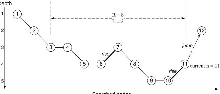
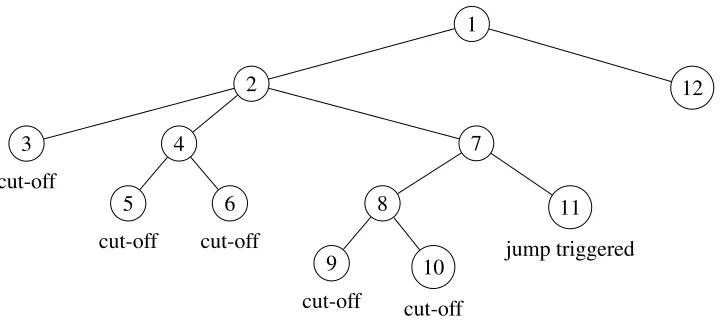
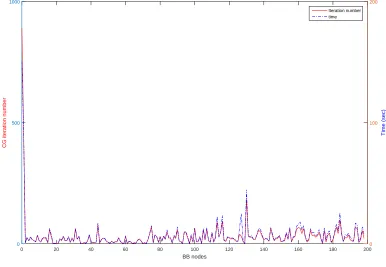
The BB search starts with depth-first. The qualities of the early nodes yielded by depth-first are often not satisfactory, as their objective values are not considered for node selection. Moreover, two cases should be noted. First, although diving is expected, depth-first search may experience oscillations trapped at the middle levels on the tree without any effective dive at all. Second, intuitively though, when the current node yields an operable solution, the probability of finding other operable solutions in its neighborhood is likely to be low. In the above two cases, a “jump” will be triggered such that depth-first is stopped temporarily and the next node to be solved will be a best active node with the smallest objective. To be specific, a jump will be triggered at a current nodenif the below is TRUE:

(noJump(n)>G)^notInDiving(n)^dBB−d(n) dBB

>εBB

_{_}

oprSol(n). (35)

In (35), noJump(n) is a counter recording how many nodes have been searched at tree noden

not in diving) and whenG=∞, it is close to depth-first. notInDiving(n)detects whether current searching is “not in diving” (returning TRUE or FALSE). Two parameters are set in determining the diving status: a backward check rangeR and a rising action limitL. To check whether depth-first searching is in diving,Rtimes of comparisons will be made among the recently searched nodes starting from nodento noden−R, i.e. theR-th earlier searched node beforen. Fori=n. . .n−R, each timenotInDiving(n)compares the depths between the pair of consecutively searched nodesiand

i−1 and if nodeihas a depth strictly higher than its former nodei−1, then a “rise” is identified. If withinRtimes of comparisons, more thanLtimes of rises are detected,notInDiving(n)will return TRUE. Note that ifR>G, thenRshould be reset toG.

Figure 1 and 2 give an example of hownotInDiving(n) determines the status at noden=11. The numbers marked inside the nodes indicate the order of how they are searched. Suppose from node 1 to node 11 depth-first is in use, the current inoperable noden=11 while in (35) the other conditions in the first disjunction term exceptnotInDiving(n) are already satisfied. Also assume thatR=8,L=2. As shown in Figure 1, there are two rises within the checking range, i.e. between

node 6 and 7, and between node 10 and 11. They are both caused by the fact that the children of node 4 and node 8 are both cut-off thus the diving cannot continue (see Figure 2). Therefore, at node 11, a jump is triggered to relocate the search to node 12 which is currently the best node in the active queue.

1

2

3 4

5 6

7

8

9 10

11 12 depth

Searched nodes 1

2

3

4

5

rise

rise jump

R = 8 L = 2

current n = 11

Figure 1: Searched nodes and their depths for thenotInDiving(n)example

The third term dBB−d(n)

dBB >εBBensures jumps will not take place whennis within anεBB-percent

distance from the BB tree’s deepest places, where the possibility of finding operable solutions is generally higher.d(n)anddBBare the depth of current nodenand the entire BB tree respectively.

The last term oprSol(n) returns to TRUE if the current node yields an operable solution and FALSE otherwise. It ensures a jump will immediately take place if an operable node has just been found.

5.3 Other technical issues of the branch-and-price solver

5.3.1 Initial feasible solutions at root: primal heuristics and naive columns

1

12 2

7

11

jump triggered 8

10

cut-off 9

cut-off 4

6

cut-off 5

cut-off 3

cut-off

Figure 2: The BB tree for thenotInDiving(n)example

turnround time) for connecting the next train at each train node. The resulting solutions are integer flows satisfying passenger demands, coupling upper bounds and coupling/decoupling time allowance while type-type compatibility and banned location restrictions are ignored. For some instances, it can provide an initial feasible solution with an acceptable quality for subsequent stages. For example, for one instance from Southern Railway with 102 trains to be served by train unit types 171/7 and 171/8, the greedy method uses 15 units while the fleet size in the manual schedule is 13 units. Note that initial feasible solutions generated by the primal heuristic often cannot provide a global upper bound at the start point for branch-and-price since requirements on type-type compatibility and banned locations are not included.

To keep the initial solution “LP-feasible” even if the number of used units exceedsbk₀ for some typek, artificial variablesβk_{≥0 associated with eachk for Constraints (17) are added with big-M} costs in the objective. To be specific, we have the following constraints

∑

yp≤bk0+βk, ∀k∈K (36)

to replace (17) and the termM∑_k∈Kβk _{is added in the objective.}

Finally when the primal heuristic cannot yield an “LP-feasible” solution, an alternative process will be invoked. It simply constructs a set of∑_j∈N|Kj|paths each containing one and only one train

j∈Nserved by one type of unit. These paths are called “naive columns” and they can always give an initial feasible solution as long as the problem is “LP-feasible”. Column management strategies are also designed to remove some or all of such naive columns beyond the root. It is often observed that naive columns yield no worse subsequent performance than the aforementioned greedy method.

5.3.2 Initial feasible solutions at leaves: column inheritance