DOI 10.1007/s10957-016-0881-6
Decomposition and Mean-Field Approach to Mixed
Integer Optimal Compensation Problems
Dario Bauso1,2 · Quanyan Zhu3 · Tamer Ba¸sar4
Received: 29 December 2014 / Accepted: 25 January 2016 / Published online: 17 February 2016 © The Author(s) 2016. This article is published with open access at Springerlink.com
Abstract Mixed integer optimal compensation deals with optimization problems with integer- and real-valued control variables to compensate disturbances in dynamic sys-tems. The mixed integer nature of controls could lead to intractability in problems of large dimensions. To address this challenge, we introduce a decomposition method which turns the originaln-dimensional optimization problem intonindependent scalar problems of lot sizing form. Each of these problems can be viewed as a two-player zero-sum game, which introduces some element of conservatism. Each scalar problem is then reformulated as a shortest path one and solved through linear programming over a receding horizon, a step that mirrors a standard procedure in mixed integer pro-gramming. We apply the decomposition method to a mean-field coupled multi-agent system problem, where each agent seeks to compensate a combination of an exoge-nous signal and the local state average. We discuss a large population mean-field type
Communicated by Benoit Chachuat.
B
Dario Bauso[email protected] Quanyan Zhu
[email protected] Tamer Ba¸sar [email protected]
1 Department of Automatic Control and Systems Engineering, The University of Sheffield,
Sheffield, UK
2 Dipartimento di Ingegneria Chimica, Gestionale, Informatica e Meccanica, Università di
Palermo, Palermo, Italy
3 Department of Electrical and Computer Engineering, Polytechnic School of Engineering New
York University, Brooklyn, NY, USA
of approximation and extend our study to opinion dynamics in social networks as a special case of interest.
Keywords Mean-field games·Optimal control·Mixed integer optimization Mathematics Subject Classification 91A13·49J35·49L20·90C11
1 Introduction
Mixed integer optimal compensation arises when optimizing a mix of integer- and real-valued control variables in order to compensate for disturbances in dynamic sys-tems. Mixed integer control can be viewed as a specific subfield of optimal hybrid control [1], addressed recently also in a receding horizon framework [2]. Optimal integer control problems have been receiving growing attention and are often cate-gorized under different names (e.g., alphabet control [3,4]). Handling integer control requires more than standard convex optimization techniques. It is known that new structural properties of the problem play important roles in mixed integer control; as an example, seemultimodularitypresented as the counterpart of convexity in discrete action spaces [5]. We should note that there is vast literature on mixed integer pro-gramming [6], and it is in this context that we cast the problem addressed in this paper. For a survey of solution methods for mixed integer lot sizing models circa early 1990s, we refer the reader to [7]. Mixed integer optimal control has been dealt with in [8–11].
1.1 Highlights of the Main Results and Relationship with the Relevant Literature
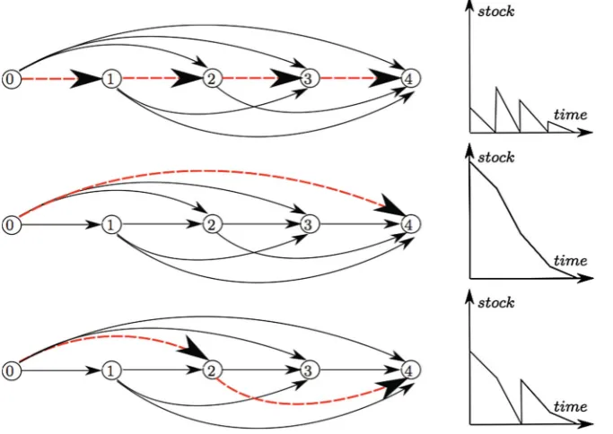
We build on existing results in the lot sizing literature that convert lot sizing problems into shortest path problems. More details on this conversion can be found in [12, p. 98] and [13,14]. The underlying idea is summarized in Fig.1, which depicts a qualitative time plot of the stock versus time (right column) for different reordering policies and associated paths (dashed arcs in figures on the left). One can use a graph where nodes correspond to periods and (solid) arcs toregeneration intervals(time intervals between consecutive orders). For a 4-period demand, thejust in timepolicy consisting of reordering at every period in order to fulfill the expected daily demand corresponds to the path (ordered sequence of nodes) traversing all the nodes, i.e.,{0,1,2,3,4} (top). The other extreme case is the one shot reordering policy where one reorders only once and at the beginning of the interval in order to fulfill the 4-period demand. The corresponding path is the single arc from node 0 to node 4, i.e.,{0,4}(middle). An intermediate policy would be to reorder at periods 0 and 2 in order to fulfill the 2-period demand. The corresponding path traverses nodes 0, 2, and 4, i.e.,{0,2,4} (bottom). In the paper, we extend this scheme to more general systems.
Fig. 1 Lot sizing problem turned into a shortest path problem: (top) just in time policy; (middle) one shot production policy; (bottom) two period production policy
can be viewed as a two-player zero-sum game, which introduces some element of conservatism. Third, we view each decomposed mixed integer problem as a shortest path problem and solve the latter through linear programming.
The conservatism arising from the robust decomposition and approximation can be reduced if we operate in accordance with the predictive control technique: (i) optimize controls for each independent system based on the prediction of other states, (ii) apply the first control, (iii) provide measurement updates of other states and re-iterate.
[image:3.439.53.395.59.301.2]We also provide in the paper a discussion on a special case of interest where each agent seeks to compensate a combination of the exogenous signal and the local state average. Here, the model is suitable to capture opinion fluctuations (sawtooth waves) insocial networks[17]. We assume that the opinion dynamics are influenced by three different factors: the media, whose influence is modeled as an exogenous signal; the presence of a stubborn agent who is able to reset other agent’s opinions; and the interactions among the agents (the endogenous factor). An underlying assumption here is that a reset for a particular agent occurs whenever that agent chooses to meet with the stubborn agent, in which case the binary control is set to one. Also, the interactions among the agents are captured by an averaging process.
In the sense above, our decomposition idea is similar to mean-field methods in large population consensus. The mean-field theory of dynamical games with large but finite populations of asymptotically negligible agents (as the population size grows to infin-ity) originated in the work of Huang et al. [18–20] and independently in that of Lasry and Lions [21–23], where the now standard terminology of mean-field games (MFG) was introduced. In addition to this, the closely related notion of Oblivious Equilibria for large population dynamic games was introduced by Weintraub et al. [24] in the framework of Markov decision processes. This theory is very versatile and is attracting an ever-increasing interest with several applications in economics, physics and biol-ogy (see [25–27]). From a mathematical point of view, the mean-field approach leads to the study of a system of partial differential equations (PDEs), where the classical Hamilton–Jacobi–Bellman equation is coupled with a Fokker–Planck equation for the density of the players, in a forward–backward fashion. The decomposition method proposed here requires that each agenti computes in advance the time evolution of the local average (see, e.g., the Fokker–Planck–Kolmogorov equation in [23,28–33]). However, since this is practically impossible, we use here the predictive control method to approximate the computation of the solution.
The main contributions of this work can therefore be summarized as follows: First, we draw a connection between game theory and a class of mixed integer control problems by decomposing ann-dimensional optimization problem intontwo-player zero-sum games. Second, by reformulating decomposed problems as shortest path problems, we show that mixed integer optimal compensation problems are tractable under certain assumptions. Third, we leverage this connection to develop a mean-field game approach to study the large-scale optimization problem using a large population game framework.
A preliminary version of this paper was presented at the 2012 American Control Conference [34]. In addition to what was presented in [34], the current paper includes a detailed analysis of the case where a large number of agents interact and this interaction is described through a state averaging process. For this case, we provide a macroscopic description of the system in terms of consensus to the average mass distribution. This part of the paper includes an additional example (Example6.3) that illustrates possible population evolutions. A further element, which is not present in [34], is an experimentally driven discussion on performance and complexity of the method provided in Example6.2.
to introducing the shortest path reformulation and the linear program. In Sect.5, we discuss the case where the local state average appears in the dynamics. In Sect.6, we present three numerical examples to illustrate the results in the paper. We conclude the paper with the recap of Sect.7.
2 Mixed Integer Optimal Compensation (MIPC)
In mixed integer optimal compensation problems, we have continuous statesx(k)∈
Rn, continuous controlsu(k)∈Rn, discrete controlsy(k)∈ {0,1}n, and continuous
disturbancesw(k)∈Rn, wherek=0,1, . . .is the time index. Evolution of the state over a finite horizon of length N is described by a linear discrete-time (difference) equation in the general form (1) below, where Aand E are matrices of compatible dimensions andx(0)=ξ0≥0 is a given initial state. Continuous and discrete controls are linked through the generalcapacity constraints(2), where the (scalar) parameter
cis an upper bound on control, with the inequalities in (1) and (2) to be interpreted component wise.
x(k+1)=Ax(k)+Ew(k)+u(k)≥0, x(N)=0, (1)
0≤u(k)≤cy(k), y(k)∈ {0,1}n. (2)
The above dynamics are characterized by one discrete and one continuous control variable per each state. Starting from nonnegative initial states, we force the state to remain confined to the positive orthant, which may describe a safety region in engi-neering applications or reflect the desire to prevent shortfalls in inventory applications. The final state,x(N), is forced to be equal to zero, which corresponds to saying that the controlu(k)has to “compensate” the cumulative effects of the disturbancesEw(k) and termAx(k)over the given horizon.
The following assumption serves to describe the common situation where the dis-turbance seeks to push the state out of the desired region. Its value is given at the beginning and fixed that way. Each column of matrix Eestablishes how each distur-bance component influences the evolution of the state vector.
Assumption 1 (Unstabilizing disturbance effects)
Ew(k) <0, (3)
where the inequality is to be interpreted component wise.
N−1
k=0
pk,u(k)
+hk,x(k)
+fk,y(k)
, (4)
where·,·denotes the Euclidean inner product. The problem of interest is thus com-pletely characterized by (1)–(4). This hybrid minimization problem can be turned into a mixed integer linear program by using the standard method discussed next. Henceforth we refer to (1)–(4) as (MIPC).
2.1 Introducing Some Structure onA
With regard to (1), we can isolate the dependence of one component state on the other ones and rewrite (1) in a way that establishes similarity with standard lot sizing models [7]:
x(k+1)=x(k)+Bx(k)+Ew(k)+u(k)≥0. (5)
Equation (5) is a straightforward representation of (1) where
B:=A−I =: {bi j}, bi j =ai j −δi j, δi j :=
1, ifi = j,
0, otherwise. (6)
To preserve the nature of the problem, which has stabilizing control actions playing against unstabilizing disturbances, we assume that the influence of other states on state
iis relatively “weak.” In other words, we assume that the influence ofBx(k)is small if compared with the unstabilizing effects of disturbances captured by the termEw(k).
Assumption 2 (Weak coupling)
Bx(k)+Ew(k) <0, (7)
where inequality is again component wise.
Essentially, the states’ mutual dependence expressed by Bx(k)only emphasizes or reduces “weakly” the destabilizing effects of the disturbances. In the next section, we present a decomposition approach that translates dynamics (5) intonscalar dynamics in “lot sizing” form [7].
3 Robust Decomposition
With the term “robust decomposition,” we mean a transformation through which dynamics (5) are replaced byn independent uncertain lot sizing models of the form (8) wherexi(k)is the inventory,di(k)the demand,ui(k)the reordered quantity and
Dk
i ⊂Rdenotes the uncertainty set:
Recall that in (5) the disturbance is given at the beginning and fixed that way. We use those values of the disturbance to determine set Dik in (8), as explained in the following. Replacing (5) with (8) is possible once we relate the demanddi(k)to the
current values of all other state components and disturbances as expressed below:
di(k)= −
n
j=1
bi jxj(k)+ n
j=1
Ei jwj(k)
= −[Bi•x(k) + Ei•w(k)],
(9)
where we denote byBi•theith row of the matrixB, with the same convention applying
toEi•. Following the decomposition, each lot sizing model is controlled by an agent
i (whose state isxi) who plays against a virtual opponent which selects a worst-case
demand, which can be viewed as atwo-player game.
Our next step is to make then dynamics in the form (8) mutually independent. Toward that end, we introduce Xk as the set of x(k) and observe that this set is bounded for boundeddi(k). The setXkcan be defined in two steps. First, we assume
that the states never leave a given region, and then we compute the worst-case vector
x(k)in the region, namely the vectorx(k)that, once substituted in (9), has the effect of pushing theith state out of the safe region. Then, we check whether the trajectory still lies within the region.
Boundedness ofXkmeans that there exists a scalarφ >0 such thatx∞≤φfor allx ∈ Xk. In view of this, it is possible to decompose the system by replacing the
current demanddi(k)by the maximal or minimal demand as computed below:
di+(k)=max
ξ∈Xk{−Bi•ξ − Ei•w(k)} =
j
[Bi j]−φ− Ei•w(k), (10)
di−(k)= min
ξ∈Xk{−Bi•ξ − Ei•w(k)} =
j
[Bi j]+φ− Ei•w(k), (11)
where[Bi j]+denotes the positive part ofBi j, i.e., max{Bi j,0}and[Bi j]−the negative
part. In the following, we will write compactlydie(k),e∈ {+,−,nil}to generically address the maximal demand (10) when e = +, the minimal demand (11) when
e= −, and the exact demand (9) whene=nil. From the above preamble, we derive the uncertainty set as
Dk
i = {η∈R: di−(k)≤η≤di+(k)}.
Likewise, (11) describes the demand that would push the state out of the positive orthant in the longest time. To complete the decomposition, it remains to transform the objective function (4) intonindependent ones:
Ji(ui,yi)= N−1
k=0
pkiui(k)+hkixi(k)+ fikyi(k)
Note that because of the linear structure of J(u,y)in (4), we have
J(u,y)=
n
i=1
Ji(ui,yi).
Thus, we have transformed the original problem into n independent mixed integer minimization problems of the form (12)–(14) below.
In the spirit of predictive control, we solve, forτ =0, . . . ,N−1, ande(τ)=nil,
e(k)=e, fork> τ,e∈ {nil,+,−}, and withξiτ being the measured state at timeτ:
(MIPCi)e min ui,yi
N−1
k=τ
pikui(k)+hkixi(k)+ fikyi(k)
(12)
xi(k+1)=xi(k)−die(k)(k)+ui(k)≥0, (13)
xi(τ)=ξiτ,xi(N)=0,
0≤ui(k)≤cyi(k), yi(k)∈ {0,1}. (14)
Note that when the superscripte=nil, we simply write(MIPCi). Denote by(MIPC)r
the relaxation of(MIPCi)where 0≤y≤1.
Lemma 3.1 The following relations hold:
(MIPCi)−, (MIPC)r ≤(MIPCi)≤(MIPCi)+.
Proof The conditions (MIPCi)− ≤ (MIPCi) ≤ (MIPCi)+ are true as di−(k) ≤
di(k)≤di+(k)for allk=0, . . . ,N−1, and the cost (12) is increasing in the demand.
The inequality (MIPC)r ≤ (MIPCi) follows from observing that in(MIPC)r we
relax the integer restrictions onyand therefore the cost cannot be higher than that in
(MIPCi).
4 Shortest Path and Linear Programming
What we will establish here is that, for the problem at hand, relaxing and massaging the problem in a certain manner leads to a shortest path reformulation of the original problem. Shortest path formulations are based on the notion of regeneration interval as discussed next.
Let us borrow from [7] the concept of regeneration interval and adapt it to the generic minimization problemidefined by (12)–(14).
Given a regeneration interval[α, β], we can define the accumulated demand over the intervaldiαβ, and the residual demandriαβ, as
diαβ= β
k=α
die(k)(k), riαβ=diαβ−
diαβ C
C. (15)
The path we take now is to reformulate problem (12)–(14) in terms of some new variables. More formally, let us consider variablesyiαβ(k)and iαβ(k)defined below with the following interpretation. Variable yαβi (k)is equal to 1 in the presence of a saturated control at timek, and 0 otherwise. Similarly, variable iαβ(k)is equal to 1 in the presence of a non-saturated control at timek, and 0 otherwise:
yiαβ(k)=
1 ui(k)=c,
0 otherwise,
αβ
i (k)=
1, 0<ui(k) <c,
0, otherwise.
Variables yiαβ(k)and iαβ(k)tell us on which period full or partial batches are ordered. Then, we can use some well-known results from the lot sizing literature to convert the original mixed integer problem (12)–(14) into a number of linear programs
LPαβi
, each one corresponding to a specific regeneration interval[α, β].
Letting eki := pki + Nj=−k1+1hij, after some standard manipulations, the linear program
LPαβi
for fixed regeneration interval[α, β]can be expressed as:
min
yα,βi ,uα,βi
β
k=α
ceki + fik
yiαβ(k)+ β
k=α
rαβeik+ fik
αβ
i (k) (16)
β
k=α
yiαβ(k)+ β
k=α
αβ
i (k)=
diαβ
c
, (17)
t
k=α
yiαβ(k)+
t
k=α
αβ
i (k)≥
diαt
c
, t =α, . . . , β−1, (18)
β
k=α
yiαβ(k)=
diαβ−riαβ c
, (19)
t
k=α
yiαβ(k)≥
diαt−riαt c
, t =α, . . . , β−1, (20)
yiαβ(k), αβi (k)≥0, k=α, . . . , β. (21)
The above model has been extensively used in the lot sizing context.
the initial and final states of a regeneration interval are null by definition. The inequality constraints (18) and (20) impose that the accumulated demand in any subinterval may not exceed the ordered quantity over the same subinterval. Again, this is due to the condition that the states are nonnegative in any period of a regeneration interval. Finally, the objective function (16) is simply a rearrangement of (12) induced by the variable transformation seen above and specialized to the regeneration interval[α, β] rather than being on the entire horizon[0,N].
The solutions of (LPαβi )that are binary are called “feasible.” We are now in a position to recall the following “nice property” of(LPαβi )presented first by Pochet and Wolsey [7].
Theorem 4.1 (Total Uni-modularity)The optimal solution of(LPαβi )is feasible.
Proof Note that the constraint matrix of
LPαβi
is a 0–1 matrix. We can reorder the constraints in a certain manner, so that the matrix has the consecutive 1’s property on each column and turns out to be totally uni-modular. It then follows thatyα,βi and iα,β
are 0–1 in any extreme solution.
4.1 Shortest Path
We now resort to well-known results on lot sizing to arrive at a shortest path model which links together the linear programming problems of all possible regeneration intervals.
Toward that end, let us define variableszαβi ∈ {0,1}, which yield 1 when a regen-eration interval [α, β] appears in the solution of (12)–(14), and 0 otherwise. The linear programming problem(LPi)solving (12)–(14) takes on the form below. For
τ =0, . . . ,N−1, solve
min
yiαβ,uαβi ,zαβi N−1
α=τ+1
N−1
β=α β
k=α
⎡
⎣ceik+ fik
yiαβ(k)+ β
k=α
rαβeik+ fik
αβ i (k) ⎤ ⎦ N
β=τ+1
zτi+1,β =1
t−1
α=τ+1
zα,i t−1−
N
β=t
zitβ =0 t =τ +2, . . . ,N,
τ +1≤α≤β ≤N β
k=α
yαβi (k)+ β
k=α
αβ
i (k)=
diαβ
c
t
k=α
yiαβ(k)+
t
k=α
αβ
i (k)≥
diαt
c
zαβi , t =α, . . . , β−1,
τ +1≤α≤β ≤N β
k=α
yiαβ(k)=
diαβ−riαβ c
zαβi τ +1≤α≤β ≤N
t
k=α
yiαβ(k)≥
diαt−riαt c
zαβi , t =α, . . . , β−1,
τ +1≤α≤β ≤N yiαβ(k), iαβ(k),zαβi ≥0, k=α, . . . , β.
The above constraints have already appeared in
LPαβi
. The only difference here
is that, now, because of the presence ofzαβi in the right-hand term, the constraints referring to a given regeneration interval come into play only if that interval is chosen as part of the solution, that is, wheneverziαβis set equal to one. Furthermore, a new class of constraints appear in the first line of the constraints. These constraints are typical of shortest path problems and in this specific case help us force the variables
zαβi (k)to describe a path from 0 toN. Finally, note that forτ =0, the linear program
(LPi)coincides with the linear program presented by Pochet and Wolsey [7].
At this point, we are in a position to recall the important result established by Pochet and Wolsey [7] and adapt it to(MIPCi)within the assumption of null final state (high
values ofhiN).
Theorem 4.2 The linear program (LPi)solves (MIPCi)with null final state.
Proof It turns out that the linear program(LPi)is a shortest path problem on variables
zα,βi . Arcs are all associated with a different regeneration interval [α, β], and the respective costs are the optimal values of the objective functions of the corresponding linear programs
LPα,βi
(cf. [7]).
4.2 Receding Horizon Implementation of(LPi)
The main difference between the lot sizing model [7] and the(LPi)arrived at here
is that in the(LPi)the initial state is non null. Actually, successive linear programs
(LPi)are linked together by the initial state condition expressed in (13), which we
rewrite below
xi(τ)=ξiτ.
diτt =max
t
k=τ
die(k)(k)−ξiτ,0
. (22)
The effective demand over an interval is the accumulated demand reduced by the inventory stored and initially available at the warehouse. From a computational stand-point, the revised expression (22) has a different effect depending on whether the accumulated demand exceeds the initial state or not, as discussed next.
1. βk=αdie(k)(k) ≥ ξiτ: the mixed linear program (MIPCi) with initial state
x(τ) = ξτ
i > 0 and accumulated demand βk=αd e(k)
i (k)is converted into an
(LPi)characterized by null initial state x(α −1) = 0 and effective demand
diαβ= βk=αdie(k)(k)−ξiτ as in the example below:
(MIPCi)
β
k=α
die(k)(k)=12, x(τ)=ξiτ =10
⇒(LPi) x(α−1)=0, diαβ=2.
2. βk=αdie(k)(k) < ξiτ: the mixed linear program (MIPCi) with initial state
x(τ)=ξτ
i >0 and accumulated demand βk=αd e(k)
i (k)is infeasible. The
solu-tion obtained at the previous periodτ −1 applies. The example below shows unfeasibility:
(MIPCi)
β
k=α
die(k)(k)=7, x(τ)=ξiτ =10
⇒(LPi)unfeasible.
5 Mean-Field Coupling
5.1 Multi-Agent System Model
Consider a graphG=(V,E)with a set of verticesV = {1, . . . ,n}and a set of edges
E ⊆V×V. Denote byNithe neighborhood of agenti, i.e.,Ni = {j ∈V :(i,j)∈E}.
We can associate with the graphGthe normalized graph Laplacian matrixL ∈Rn×n
whosei j-th entry is
li j =
−1
|Ni|, j ∈ Ni,
1, j =i.
Now, a special case of interest is whenBin (5) isB= − L for some sufficiently small scalar >0. In this case, dynamics (5) become:
x(k+1)=x(k)− L x(k)+Ew(k)+u(k)≥0. (23)
Essentially, the above dynamics together with the constraint x(N) = 0 arise in all those situations where each agenti =1, . . . ,ntries to compensate a combination of the exogenous signalw(k)and the local state average given by
¯ mi(k)=
1
|Ni|
j∈Ni
xj(k).
Elaborating along the line of the robust decomposition (8), we can then compute the disturbance taking into account the influence of the local average on the exogenous signal as follows:
di(k)= −[ (m¯i(k)−xi(k))+ Ei•, w(k)].
Note that Assumption2in this case says that the exogenous signal is dominant if compared to the weak influence from neighbors.
In principle, for the decomposition method to be exact, each agenti should know in advance the time evolution of the local averagem¯i(k), fork=0, . . . ,N. However, this
may not be feasible. One way to approximate the local averagem¯i(k)is through
mean-field methods. Under the further assumption that the number of agents is large and the agent dynamics are symmetric, the local average can be characterized through the finite-difference approximation of the continuity or advection equation that describes the transport of a conserved quantity [35]. Another way to deal with the problem is to use the predictive control method to approximate the computation. More specifically, when we solve the problem over the horizon fromk˜≥0 toN, we assume that neighbor agents communicate their state and so at least the first samplem¯i(k)˜ is exact. In the
later stages of the horizon, each agent approximates the local average by specializing (10)–(11) to our case. Note that maximal and minimal demand can be obtained by assuming that all agents j =iare in 0 orφ, respectively, and thus we have for agent
i:
Alternatively, this also corresponds to assuming for the uncertain setDikthe following expression:
Dk
i = {η∈R: − (φ−xi)− Ei•, w(k) ≤η≤ xi− Ei•, w(k)}.
The above set up includes the case where agents are homogeneous as explained next.
5.2 Homogeneous Agents
Within the realm of mean-field coupling, a particularly interesting case is the one where agents are homogeneous in the sense that they behave similarly when at the same state. For these problems, a main question is the asymptotic population behavior, i.e., the behavior of the population when the number of agents is large.
Suppose that all agents face the same disturbance comprised of a constant value plus a random walk, i.e.,ωi(k):= Ei•w(k)= const.+σiγi(k)whereγi(k)is the
random walk, andσi is the random walk coefficient, for all agentsi.
Denoting the saturation function by
sat[x] = ⎧ ⎨ ⎩
x+, ifx>x+, x−, ifx<x−, x, ifx−≤x≤x+,
(24)
the system dynamics takes the form
xi(k+1)=xi(k)−di(k)+ui(k),
di(k)= −[sat[ (m¯i(k)−xi(k))] +ωi(k)], (25)
whereui(k)is an(s,S)strategy (see, e.g., [36]) of the type
ui(k)=
S−xi(k) ifxi(k)±ε≤s,
0 otherwise. (26)
Essentially, the control restores the original upper thresholdS anytime when the stocked inventory (the state) goes below a lower thresholds. Such a policy has been proven to be optimal in the presence of fixed costs in a number of inventory appli-cations. Note that the saturation function is used here only to avoid state oscillations when the agents are far enough from the local average.
Our goal is now to provide a macroscopic description of the system and analyze the corresponding behavior. To do this, we borrow from [37] a modeling approach based on stochastic matrices. LetW =I− Lbe a row stochastic matrix, i.e.,W1=1. The system Eq. (23) can be rewritten as
x(k+1)=W x(k)+ωi(k)+u(k).
the average the following recursive equation:
¯
m(k+1)= 1
n1,x(k+1) =
1
n1,W x(k)+ω(k)+u(k) = ¯m(k)+1
n1, ω(k)+u(k), (27)
whereω(k)is the vector whoseith component isωi(k).
The above is a stochastic process whose first-order moment is generated by
Em(k¯ +1)=Em(k)¯ +const.+1
n1,u(k),
Em¯(0)=n
i=1xi(0). (28) Now, our aim is to analyze the convergence of the agents’ opinions to their average. Toward that end, defineM= 1n1⊗1. Then for a given vectorx(k), we haveMx(k)= (1
n1⊗1)x(k)= ¯m(k)1. With the above in mind, the deviation of each agent statexi(k)
from the averagem(k)¯ is captured by the vector
z(k):=x(k)−Mx(k)=(I−M)x(k).
If agents reach average-consensus, i.e., their opinions all converge to the average, then the variable z(k)goes to zero. After some transformations, we obtain forz(k)the following iteration:
z(k+1)=(I−M)(W x(k)+ω(k)+u(k))
=(W −M)(I−M)x(k)+(I −M)(ω(k)+u(k)) =(W −M)z(k)+(I −M)(ω(k)+u(k)).
Following a few recursions, we can relatez(k)to the initial discrepancy valuez(0) and to the sequence of inputsω(k)andu(k)as follows:
z(k)=(W−M)kz(
0)+
k−t−1
t=0
(I−M)(ω(k)+u(k)).
Now,z(k)=(W−M)kz(0)is a typical averaging rule and we know that it converges to the average ifW −M < 1, where we denote byW −Mthe spectral or maximum singular value norm of the matrixW−M[37]. In the absence of Brownian motions, the agents can still reach consensus or at leastε-consensus (εis convergence tolerance) as established in the following result.
Theorem 5.1 (Controlled invariance)Letσi =0for all i andW−M<1. If there
Proof First, note that fromσi = 0 for alli and homogeneity it follows that(I −
M)ω(k)=0 for allk. Now, observe that ifz(τ) ≤εthen(I−M)u(k)≈0. This also means that
∞
k=0
(I−M)u(k)2=τ− 1
k=0
(I −M)u(k)2<∞, lim
k→∞(I−M)u(k)
2= 0.
The above uses the fact that(I −M)u(k)2is bounded for allkand implies that the sequence{z(k)}is convergent. Now, let us consider the subsequence{ζ(k)}where
ζ(k)=z(τ+k). We know that{ζ(k)}follows the equationζ(k)=(W −M)kζ(0) and fromW −M < 1 it converges to zero. Since{z(k)}is convergent and the subsequence{ζ(k)}converges to zero, we can conclude that{z(k)}converges to zero
as well.
Example 5.1 For a givenx(0)we can compute the first time that a controluiis set to 1.
Let us denote this time byt˜. We can also computeτ =min{k>0| (W−M)kz(0) ≤
ε}and check thatτ ≤ ˜t. If the latter condition holds true, then the above theorem applies and opinions of all agents evolve according to the periodic law (27) ofm(k)¯ and reach consensus to the average.
6 Numerical Examples
In this section, we present three numerical examples to illustrate the findings in the paper.
6.1 Second-Order Dynamics
Example 6.1 In this specific example, dynamics (1) take the form given below in (29). Such dynamics are particularly significant as they reproduce the typical interaction between position and velocity in a sampled second-order system. Initial and final states are null,x(0)=x(N)=0, and state values must remain in the positive quadrant for all time. More specifically, denoting byx1(k)the position andx2(k)an opposite in sign velocity, the dynamics appear as:
x1(k+1)
x2(k+1)
=
1 −κ
κ 1
x1(k)
x2(k)
−
w1(k)
w2(k)
+
u1(k)
u2(k)
≥0. (29)
A closer look at the first equation reveals that a higher velocity x2(k) leads to a faster decrease of position x1(k+1). Similarly, the second equation tells us that a higher positionx1(k)induces a faster increase of velocityx2(k+1)because of some elastic reaction. In both equations, the positive disturbances,wi(k) >0 seek to push
the statesxi(k+1)out of the positive quadrant. Their effect is counterbalanced by
positive control actionsui. Also, acting on parameterκ we can easily guarantee the
Turning to the capacity constraints (2), for this two-dimensional example, these constraints can be rewritten as:
0≤
u1(k)
u2(k)
≤C
y1(k)
y2(k)
,
y1(k)
y2(k)
∈ {0,1}2.
Regarding the objective function (4), we consider the case where fixed costs are much more relevant than the proportional and holding ones. This results in choosing a high value for fk in comparison with values of parameters pk,hk as shown in the next linear objective function where1nindicates the n-dimensional row vector on 1’s:
J(u,y)=
N−1
k=0
1n,u(k) + 1n,x(k) +1001n,y(k). (30)
This choice makes sense for two reasons. First, all the work is centered around issues deriving from the integer nature of y(k). So, high values of fk emphasize the role of integer variables in the objective function. Second, high fixed costs lead to solu-tions with the fewest number of control acsolu-tions and this facilitates the validation and interpretation of the simulated results.
Next, we decompose dynamics (29) in scalar lot sizing form (13) which we rewrite below:
xi(k+1)=xi(k)−die(k)(k)+ui(k).
As regards the estimated demanddi+, a natural choice is to setdi+as below, where we have denoted by x˜1(k)(respectively, x˜2(k)) the estimated value of state x1(k) (respectively,x2(k)) in the dynamics ofx2(k)(respectively,x1(k)):
d1+(k) d2+(k)
=
0 κ
−κ 0
˜ x1(k)
˜ x2(k)
+
w1(k)
w2(k)
. (31)
Now, the question is: Which expression should be used to represent the set of admis-sible state vectors,Xk, appearing in equation (10)? A possible answer is given next:
˜
x1(k+1)
˜
x2(k+1)
=
˜ x1(k)
˜ x2(k)
+
0
κx¯1
−
0
w2(k)
+ 0 C , ˜ x1(0)
˜ x2(0)
=
x1(0)
˜ x2(0)
. (32)
0 5 10 15 20 10−2
10−1 100 101 102
N
sec
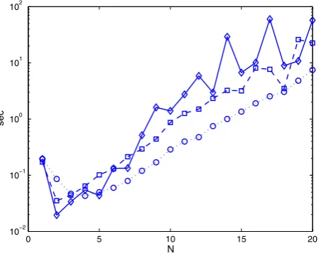
Fig. 2 Average computational time versus horizon lengthNof the mixed integer predictive control problem (solid diamonds), of the decomposed problem(MIPCi)(dashed squares), and of the linear program(LPi)
(dotted circles)
in the second equation of (31). We now observe a negative contribution of the term
−κx˜1(k)ond2+(k)and therefore take forx˜1(k)a possible lower bound of x1(k)as shown in the first equation of (32).
We can now move to show and comment on our simulated results.
We have carried out two different sets of experiments. In the line of the weakly coupling assumption (see Assumption 2), we have set κ small enough and in the range from 0.01 to 0.225. Such a range works well as we will see that|κxi|is always
less thanwi, which also meansBx(k)+Ew(k) <0. For the sake of simplicity and
without loss of generality, we take capacityC=3, disturbanceswi =1 andx¯1=1. Unitary disturbances facilitate the validation and interpretation of the results as the accumulated demand over the horizon turns to be very close to the horizon length. The two experiments differ also in the horizon length N for reasons to be clarified next. All simulations were carried out with MATLAB on an Intel(R) Core(TM)2 Duo CPU P8400 at 2.27 GHz and a 3 GB of RAM.
The first set of experiments aims at analyzing the computational benefits of the decomposition and relaxation upon which our solution method is based. So, we con-siderκ =0.1 and horizon lengths N =1, . . . ,10. We do not need to consider larger values ofNas even in this small range of values, the differences in the computational times are already sufficiently evident as clearly illustrated in Fig.2. Here, we plot the average computational time versus the horizon lengthsNof the mixed integer predic-tive control problem (solid diamonds), of the decomposed problem(MIPCi)(dashed
squares) and of the linear program(LPi)(dotted circles). Average computational time
means the average time one agent takes to make a single decision (the total time is about 2N times the average one). As it can be seen, the computational time of the linear program(LPi)is a fraction either of the one required by the (MIPC) or of the
[image:18.439.109.334.57.237.2]0 0.05 0.1 0.15 0.2 0.25 0
2 4 6 8 10 12 14 16 18 20
elastic coefficient
percentage error
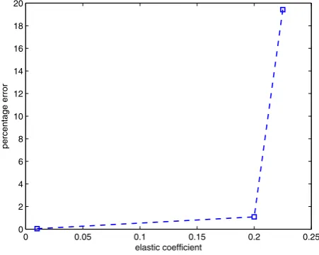
Fig. 3 Percentage error % for different values of the elastic coefficientκ
In a second set of simulations, for a horizon length N = 6, we have studied how the percentage error below varies with different values of the elastic coefficient
κ = {0.01, 0.2,0.225}:
%=optimal cost of(MIPCi)−optimal cost of (MIPC) optimal cost of (MIPC) %.
The role ofκis crucial as we recall thatκdescribes the effective tightness and coupling between different statesx1(k)andx2(k). We do expect that small values for coefficient
κ, which means weak coupling of state components, may lead to small errors %. Differently, high values ofκ, describing a strong coupling between state components, are supposed to induce higher values of %.
This is in line with what we can observe in Fig.3where we plot the error % as a function of coefficientκ. For relatively small values ofκ in the range from 0 to 0.2, we observe a percentage error not exceeding 1 %, %≤1. A discontinuity at around
κ =0.2 causes the error % to go from about 1–20 %.
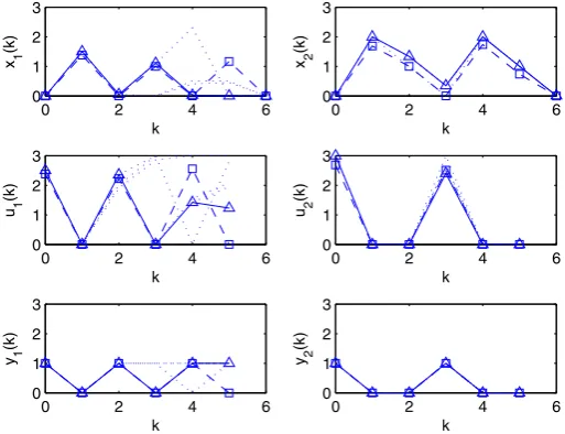
In Fig.4, for a horizon lengthN =6 and for a value ofκ =0.225, we depict the exact solution (dashed squares) and approximate solution (solid triangles) returned by the (MIPC) and by the(LPi), respectively. Dotted lines represent predicted trajectories
in earlier periods of the receding horizon. We note that controlsui(k)never exceed
the capacity and are always associated with unitary control actions yi(k). Also, we
observe four control actions (four peaks at 1) in the approximate solution and three in the exact solution. So we have an increase in the percentage error, of 20%. A last observation concerning the exact plot of yi(k)is that the number of control actions
[image:19.439.106.332.57.237.2]0 2 4 6 0
1 2 3
x 1
(k)
k
0 2 4 6
0 1 2 3
x 2
(k)
k
0 2 4 6
0 1 2 3
u 1
(k)
k
0 2 4 6
0 1 2 3
u 2
(k)
k
0 2 4 6
0 1 2 3
y 1
(k)
k
0 2 4 6
0 1 2 3
y 2
(k)
k
Fig. 4 Elastic coefficientκ=0.225. Exact solution (dashed squares) and approximate solution (solid tri-angles) returned by the mixed integer linear program (MIPC) and by the linear program(LPi), respectively.
Horizon length isN=6. Time plot of statesxi(k), continuous controlsui(k)and discrete controlsyi(k)
We also compared exact and approximate solutions for a smaller value ofκ =0.2 and observed that we still have notable differences in the plot of continuous controls
u1(k)which cause a reduced percentage error % = 1. We have concluded our simulations by noticing that the percentage error % is around zero when we reduce further the value ofκ to 0.01.
6.2 Numerical Examples on the Mean-Field
In this subsection, we present two numerical examples on the mean-field approxima-tion.
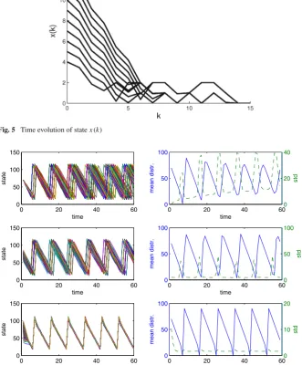
Example 6.2 Consider a complete network ofn=10 agents. The local state average is the same for all i and also is equal to the global average, i.e., for alli it holds thatm¯i(k)= 1n j∈V,j=i(xj(k)−xi(k)). The horizon length isN =15, the scalar
=0.1, the initial state isx(0)= [4. . .13], and the disturbance isEi•w(k)=1 if
kis odd andEi•w(k)=2 otherwise for all agentsi. The bound on input isC =3,
and the objective function is given below where1n indicates then-dimensional row vector on 1’s:
J(u,y)=
N−1
k=0
1n,u(k)+1n,x(k)+1001n,y(k). (33)
[image:20.439.91.348.57.254.2]Fig. 5 Time evolution of statex(k)
0 20 40 60
0 50 100 150
state
time
0 50 100
mean distr.
time
0 20 40 600
20 40
std
0 20 40 60
0 50 100 150
state
time
0 50 100
mean distr.
time
0 20 40 600
50 100
std
0 20 40 60
0 50 100 150
state
time
0 50 100
mean distr.
time
0 20 40 600
10 20
std
Fig. 6 Population evolution for values of the averaging parameter =10−4,10−1,1 and initial sparsity std= 10−1,5,10 (from top to bottom): (left) time plot of statex(k); (right) average distribution and standard deviation
[image:21.439.53.385.104.505.2]0 20 40 60 80 100 120 0
0.5 1
distr.
0 20 40 60 80 100 120
0 0.05 0.1 0.15 0.2
distr.
0 20 40 60 80 100 120
0 0.1 0.2 0.3 0.4
state
distr.
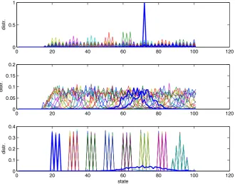
Fig. 7 Distribution for increasing values of the averaging parameter =10−4,10−1,1 and initial sparsity std= 10−1,5,10 (from top to bottom)
The horizon length is N = 60, the scalar = 10−4,10−1,1, and the initial state
x(0)is extracted from a Gaussian distribution with mean 70 and standard deviation
st d=10−1,5,10. The disturbance isEi•w(k)=10+2γi(k)whereγi(k)is a random
walk, for all agentsi. Thus, the system dynamics take the form
xi(k+1)=xi(k)−di(k)+ui(k),
di(k)= −[sat[ (m¯i(k)−xi(k))] +10+2γi(k)], (34)
whereui(k)is an(s,S)strategy of the type
ui(k)=
100, ifxi(k)±ε≤20,
0, otherwise. (35)
[image:22.439.56.387.56.314.2]Figure7shows the population distribution for each one of the above simulations (from top to bottom). Thick lines highlight initial and final distributions.
7 Conclusions
In a nutshell, we have proposed a robust decomposition method which brings ann -dimensional hybrid optimization problem intonindependent tractable scalar problems of lot sizing form. Through examples, we have illustrated the mean-field coupling in a multi-agent system problem, where each agent seeks to compensate a combination of an exogenous signal and the local state average. We have discussed a large population mean-field type of approximation as well as the application of predictive control methods.
There are at least three possibilities for future developments. First, one needs to study connections between regeneration intervals and reverse dwell time condi-tions developed in hybrid/impulsive control. Second, we intend to zoom in on the exploitation of cutting plane methods to increase the efficiency of linear relaxation approximations. Third, it would be of interest to investigate the mean-field large pop-ulation approximations that arise from the decomposition of the mixed integer optimal compensation problem.
Acknowledgments The work of D. Bauso was supported by the 2012 “Research Fellow” Program of the Dipartimento di Matematica, Università di Trento and by PRIN 20103S5RN3 “Robust decision making in markets and organizations, 2013–2016.” The work of T. Ba¸sar was supported in part by the U.S. Air Force Office of Scientific Research (AFOSR) under MURI Grant FA9550-10-1-0573 and in part by NSA through the Information Trust Institute at the University of Illinois.
Open Access This article is distributed under the terms of the Creative Commons Attribution 4.0 Interna-tional License (http://creativecommons.org/licenses/by/4.0/), which permits unrestricted use, distribution, and reproduction in any medium, provided you give appropriate credit to the original author(s) and the source, provide a link to the Creative Commons license, and indicate if changes were made.
References
1. Branicky, M.S., Borkar, V.S., Mitter, S.K.: A unified framework for hybrid control: model and optimal control theory. IEEE Trans. Autom. Control43(1), 31–45 (1998)
2. Axehill, D., Vandenberghe, L., Hansson, A.: Convex relaxations for mixed integer predictive control. Automatica46(9), 1540–1545 (2010)
3. Goodwin, G., Quevedo, D.: Finite alphabet control and estimation. Int. J. Control Autom. Syst.1, 412–430 (2003)
4. Tarraf, D.C., Megretski, A., Dahleh, M.A.: A framework for robust stability of systems over finite alphabets. IEEE Trans. Autom. Control53(5), 1133–1146 (2008)
5. Waal, P.R.D., Schuppen, J.H.V.: A class of team problems with discrete action spaces: optimality conditions based on multimodularity. SIAM J. Control Optim.38, 875–892 (2000)
6. Nemhauser, G.L., Wolsey, L.A.: Integer and Combinatorial Optimization. Wiley, New York (1988) 7. Pochet, Y., Wolsey, L.A.: Lot sizing with constant batches: formulations and valid inequalities. Math.
Oper. Res.18(4), 767–785 (1993)
8. Pochet, Y., Wolsey, L.A.: Production Planning by Mixed Integer Programming. Springer Series in Operations Research and Financial Engineering. Springer, New York (2006)
10. Sager, S., Bock, H.G., Reinelt, G.: Direct methods with maximal lower bound for mixed-integer optimal control problems. Math. Program. A118(1), 109–149 (2009)
11. Sager, S., Claeys, M., Messine, F.: Efficient upper and lower bounds for global mixed-integer optimal control. J. Glob. Optim.61(4), 721–743 (2015)
12. Ahuja, R., Magnanti, T., Orlin, J.: Network Flows: Theory, Algorithms, and Applications. Prentice Hall, Englewood Cliffs (1993)
13. Imai, H., Iri, M.: Computational–geometric methods for polygonal approximations of a curve. Comput. Vis. Graph. Image Process.36(1), 31–41 (1986)
14. Imai, H., Iri, M.: An optimal algorithm for approximating a piecewise linear function. J. Inf. Process. 9(3), 159–162 (1987)
15. Bauso, D.: Boolean-controlled systems via receding horizon and linear programing. Math. Control Signals Syst. (MCSS)21(1), 69–91 (2009)
16. Hespanha, J., Liberzon, D., Teel, A.: Lyapunov characterizations of input-to-state stability for impulsive systems. Automatica44(11), 2735–2744 (2008)
17. Acemo˘glu, D., Como, G., Fagnani, F., Ozdaglar, A.: Opinion fluctuations and disagreement in social networks. Math. Oper. Res.38(1), 1–27 (2013)
18. Huang, M., Caines, P., Malhamé, R.: Individual and mass behaviour in large population stochastic wireless power control problems: centralized and Nash equilibrium solutions. In: Proceedings 42nd IEEE Conference on Decision and Control, Maui, HI, pp. 98–103 (2003)
19. Huang, M., Caines, P., Malhamé, R.: Large population stochastic dynamic games: closed loop Kean– Vlasov systems and the Nash certainty equivalence principle. Commun. Inf. Syst.6(3), 221–252 (2006) 20. Huang, M., Caines, P., Malhamé, R.: Large population cost-coupled LQG problems with non-uniform agents: individual-mass behaviour and decentralized -Nash equilibria. IEEE Trans. Autom. Control 52(9), 1560–1571 (2007)
21. Lasry, J., Lions, P.: Jeux à champ moyen. i le cas stationnaire. C. R. Math.343(9), 619–625 (2006) 22. Lasry, J., Lions, P.: Jeux à champ moyen. ii horizon fini et controle optimal. C. R. Math.343(10),
679–684 (2006)
23. Lasry, J., Lions, P.: Mean field games. Jpn. J. Math.2, 229–260 (2007)
24. Weintraub, G.Y., Benkard, L., Van Roy, B.: Oblivious equilibrium: a mean field approximation for large-scale dynamic games. In: Weiss, Y., Schölkopf, B., Platt, J.C. (eds.) Advances in Neural Information Processing Systems 18, pp. 1489–1496. MIT Press, Cambridge (2006).http://papers.nips.cc/paper/ 2786-oblivious-equilibrium-a-mean-field-approximation-for-large-scale-dynamic-games.pdf 25. Achdou, Y., Camilli, F., Dolcetta, I.C.: Mean field games: numerical methods for the planning problem.
SIAM J. Control Optim.50, 77–109 (2012)
26. Gueant, O., Lasry, J., Lions, P.: Mean field games and applications, chap. Paris-Princeton Lectures, pp. 1–66. Springer (2010)
27. Lachapelle, A., Salomon, J., Turinici, G.: Computation of mean field equilibria in economics. Math. Models Methods Appl. Sci.20, 1–22 (2010)
28. Achdou, Y., Dolcetta, I.C.: Mean field games: numerical methods. SIAM J. Numer. Anal.48, 1136– 1162 (2010)
29. Bauso, D., Tembine, H., Ba¸sar, T.: Robust mean field games. Dyn. Games Appl. (2015). doi:10.1007/ s13235-015-0160-4
30. Tembine, H., Zhu, Q., Ba¸sar, T.: Risk-sensitive mean-field stochastic differential games. In: Proceedings of 2011 IFAC World Congress, Milan, Italy (2011)
31. Tembine, H., Zhu, Q., Ba¸sar, T.: Risk-sensitive mean-field games. IEEE Trans. Autom. Control59(4), 835–850 (2014)
32. Zhu, Q., Tembine, H., Ba¸sar, T.: Hybrid risk-sensitive mean-field stochastic differential games with application to molecular biology. In: Proceedings of Conference on Decision and Control, Orlando, FL (2011)
33. Zhu, Q., Ba¸sar, T.: A multi-resolution large population game framework for smart grid demand response management. In: International Conference on Network Games, Control and Optimization (NETG-COOP 2011), Paris, France (2011)
34. Bauso, D., Zhu, Q., Ba¸sar, T.: Mixed integer optimal compensation: decompositions and mean-field approximations. In: Proceedings of 2012 American Control Conference, Montreal, CA, pp. 2663–2668 (2012)
36. Clark, A., Scarf, S.: Optimal policies for a multi-echelon inventory problem. Manag. Sci.6(4), 475–490 (1960)