Effects of environmental variables on invasive amphibian activity: using model selection on quantiles for counts

using model selection on quantiles for counts

1

Centre for Tropical Biodiversity and Climate Change, College of Science and Engineering, James Cook University, Townsville, Queensland 4814 Australia

2

U.S. Geological Survey, Fort Collins Science Centre, 2150 Centre Ave, Bldg C, Fort Collins, Colorado 80526 USA

Citation:Muller, B. J., B.S. Cade, and L. Schwarzkopf. 2018. Effects of environmental variables on invasive amphibian activity: using model selection on quantiles for counts. Ecosphere 9(1):e02067. 10.1002/ecs2.2067

Abstract. Many different factors influence animal activity. Often, the value of an environmental variable may influence significantly the upper or lower tails of the activity distribution. For describing relationships with heterogeneous boundaries, quantile regressions predict a quantile of the conditional distribution of the dependent variable. A quantile count model extends linear quantile regression methods to discrete response variables, and is useful if activity is quantified by trapping, where there may be many tied (equal) values in the activity distribution, over a small range of discrete values. Additionally, different environ-mental variables in combination may have synergistic or antagonistic effects on activity, so examining their effects together, in a modeling framework, is a useful approach. Thus, model selection on quantile counts can be used to determine the relative importance of different variables in determining activity, across the entire distribution of capture results. We conducted model selection on quantile count models to describe the factors affecting activity (numbers of captures) of cane toads (Rhinella marina) in response to several environmental variables (humidity, temperature, rainfall, wind speed, and moon luminosity) over eleven months of trapping. Environmental effects on activity are understudied in this pest animal. In the dry sea-son, model selection on quantile count models suggested that rainfall positively affected activity, especially near the lower tails of the activity distribution. In the wet season, wind speed limited activity near the max-imum of the distribution, while minmax-imum activity increased with minmax-imum temperature. This statistical methodology allowed us to explore, in depth, how environmental factors influenced activity across the entire distribution, and is applicable to any survey or trapping regime, in which environmental variables affect activity.

Key words: animal activity; cane toad; model selection; quantile count model; quantile regression; Rhinella marina.

Received9 November 2017; accepted 14 November 2017. Corresponding Editor: Debra P. C. Peters.

Copyright:©2018 Muller et al. This is an open access article under the terms of the Creative Commons Attribution License, which permits use, distribution and reproduction in any medium, provided the original work is properly cited.

 E-mail: [email protected]

I

Animal activity is influenced by a complex web of factors (Tester and Figala 1990), including a range of environmental variables (Chamaill e-Jammes et al. 2007, Upham and Hafner 2013). Animal activity can vary widely in response to a variety of different environmental variables, but rather than determining the mean number of active animals, such variables may impose a limit

Quantile regression is especially useful for exam-ining distributions with heterogeneous variances (Koenker and Bassett 1978), a common character-istic of distributions in ecology (Cade and Noon 2003), including animal activity in relation to environmental variables (Johnson et al. 2014). Specifically, rates of change near the maximum (i.e., 0.95 quantile) or minimum (i.e., 0.05 quan-tile) of the distribution are often a better repre-sentation of the influence of the measured variable than the mean (Thomson et al. 1996, Cade et al. 1999). If, for example, a particular measured variable imposes a limit on activity, the organism’s response cannot increase to more than the upper limit set by that factor; however, it can be any value less than that, for example, if other, unmeasured, factors are also influencing activity (Cade and Noon 2003).

Our motivating example was estimating effects of various environmental variables on cane toad (Rhinella marina) activity in northern Australia. Cane toads are large, nocturnal, terrestrial anu-rans originating from South America, whose invaded range includes many tropical and sub-tropical areas globally, including Australia. The physiological constraints on terrestrial amphib-ians (Tracy 1976), and experimental data on cane toads (e.g., Cohen and Alford 1996), suggest that seasonal variation in activity should be strongly associated with environmental moisture. Wind speed also affects desiccation rates, and activity, of anurans (Henzi et al. 1995), while locomotor performance and behavior are strongly depen-dent on temperature in ectotherms (Huey and Stevenson 1979, Huey 1982). Finally, positive and negative effects of lunar cycles on amphibian biology have also been observed (Grant et al. 2012). These factors limit activity in other species; for example, several ectothermic species are inac-tive below certain temperatures (e.g., Lei and Booth 2014). Any combination of these environ-mental variables may impose a limit on the maxi-mum or minimaxi-mum activity of cane toads.

Trapping is a common method for measuring animal activity (e.g., Gibbons and Bennett 1974, Price 1977, Rowcliffe et al. 2014) and could be used to measure cane toad activity (Muller and Schwarzkopf 2017). Cane toad traps for adults contain a lure that produces a cane toad adver-tisement call, and a light that attracts insects as a visual cue (Yeager et al. 2014). Trap efficacy

depends primarily on activity; toads must be active to approach the lure, and enter the trap. Therefore, the number of toads trapped per night provides an estimate of toad activity on that night. However, if captures are low, or if the trap has limited capacity (i.e., the maximum number of animals capturable is constrained by trap size), trapping may result in a very small range of counts, with numerous tied (equal) count val-ues. Indeed, previous studies report mean cane toad capture rates of approximately 1–6 individ-uals per trap per night, and it is uncommon to exceed 14 captures in a single night (although the maximum number of toads caught in a single trap to date was 31; Muller and Schwarzkopf 2017). In this case, conventional quantile regres-sion analysis creates serious interpretation and inference issues, because the models assume a continuous dependent variable, rather than a dis-crete dependent variable (Cade and Dong 2008). The quantile count model is a special implemen-tation of conventional quantile regression, whereby the changes in quantiles of counts are estimated by making them continuous random variables and then back-transforming estimates to the discrete response without sacrificing model accuracy (Machado and Santos Silva 2005). Therefore, a quantile count model can be used to analyze trapping data, to examine the entire cane toad activity distribution in response to an environmental variable.

respect to a null model with just an intercept, then the comparison of differences in AIC is related to the proportionate reduction in varia-tion of the phenomenon explained by each com-bination of variables (adjusted by the number of estimated parameters), given what was mea-sured (Richards et al. 2011). Akaike’s information criterion is calculated using the number offitted parameters (including the intercept) in the model and the likelihood associated with the maxi-mum-likelihood estimate. The weighted sums of absolute deviations minimized in conventional quantile regression estimation are maximum-likelihood estimates assuming an asymmetric double exponential distribution, providing the basis for computing AIC and other information criteria on quantile regression models (Koenker and Machado 1999, Yu and Moyeed 2001, Cade et al. 2005). Therefore, model selection on quan-tile count models can be used to determine which combination of variables affects toad activity across the entire response distribution.

We trapped cane toads over eleven months at one location while simultaneously collecting infor-mation on humidity, temperature, rainfall, wind speed, and moon luminosity. We examined the distributions of toad captures using model selec-tion on quantile count models (using every 5th quantile betweens= 0.05 ands= 0.95) to exam-ine which environmental variables affected toad activity at different parts of the activity distribu-tion during different seasons. We suggest that model selection on quantile count models is appli-cable to any trapping regime for which several environmental variables affect the number of indi-viduals captured, especially if those effects occur near the lower or upper tails of the distribution.

M

M

Study site

The study occurred on Orpheus Island (18°360_{46.0″S, 146°29}0_{25.2″E) from 21 May 2013} to 28 March 2014, with the exception of 16 d in November 2013, 17 d in December 2013, 10 d in January 2014, and 9 d in February 2014. The island is approximately 23 km east of the Australian mainland and 120 km north of Townsville, Queensland. It is approximately 12 km long and is comprised primarily of dry woodlands, with rainforest patches.

Data collection

To catch toads, we used wire traps (191 9 0.25 m), equipped with doors that opened easily with pressure from outside, but prevented egress of trapped toads. The trap con-tained a lure that repeatedly played a cane toad advertisement call at night, and had a small LED black (UV) light that attracted insects. More detail on the trap and methodology is available in Yeager et al. (2014).

We used two traps for the study, at two trap-ping sites. Both traptrap-ping sites were located in open, grassy areas and had similar ambient light (x = 0.051 lx) and environmental noise (x = 32.5 dB) levels. We measured light and noise levels at each site on 15 randomly selected nights, at 22:00 hours, using a lux meter (ATP DT-1300), and a C-weighted Lutron sound level meter (model: SL-4013). We placed the traps 400 m apart, such that the acoustic lure at one site could not be heard by toads at the other site (Muller et al. 2016). We removed, counted, and sexed trapped toads daily by visual inspection of coloration and skin texture (females are dark brown with a smooth bumpy dorsum, whereas males are lighter with a rough sandpapery dor-sum). We placed a water bowl and PVC pipe for shelter in each trap. Toads were euthanized immediately after their removal from the traps, using an overdose (350 ppm) of buffered tricaine methanesulfonate (MS-222), and exposure was via submersion in water containing a sodium bicarbonate-buffered solution. Euthanizing toads after capture may have reduced the number of toads available for capture on subsequent nights, but there was never a decrease in toad numbers that was not easily explained by weather (e.g., there were no consistent patterns in which nightly captures were low following a large capture event). Toads move nomadically (Sch-warzkopf and Alford 2002), and the size of the toad population, and the island, facilitated con-stant immigration into the study area, and there-fore, the number of toads available to local trapping was likely approximately constant.

every night during the trapping period. We aver-aged half-hourly recordings across the 12-h per-iod from 18:00 hours to 6:00 hours to calculate nightly averages. We characterized moon lumi-nosity as the percent of the moon illuminated on each night (as measured from Townsville; approximately 79 km from the study site) during the trapping period (obtained from www.timea nddate.com).

Statistical methods

We divided the trapping period into four sea-sons: the dry season (June–August), the pre-wet season (September–November), the wet season (December–February), and the post-wet season (March–May).

We used captures for each trap from each night as replicates so each night had two mea-sures of toad activity which were counts of cap-tured toads. We used the quantile count model of Machado and Santos Silva (2005), where the dis-crete count response (y) is transformed to the continuous scale (jittered) for quantile estimates by adding a random uniform number between 0 and 1 to each count,z= y + U[0, 1). We used an exponential count model,Qz(s|X)= s+exp(Xb(s)), estimated in its linear form by taking loga-rithms, for log(zs) theQlog(z s)(s|X)= Xb(s), whereXis the matrix of predictor variables and a column of 1’s for the intercept. Estimates in the artificial continuous scale are then back-transformed with a ceiling function, Qy(s|X)= dsþexpðX^bðsÞÞ 1 e, to recover the quantile estimates in the discrete random variable scale (counts y). Our quantile count model had the typical multiplicative exponential form used with other parametric count models (Cade and Dong 2008) that ensures that all estimates are greater than or equal to zero. For each season, we estimatedfive candidate quantile count mod-els with environmental predictors (humidity, minimum temperature, rainfall, wind speed, and moon luminosity) and one null quantile count model with just an intercept. Estimates were implemented with the rq() function in the quan-treg package for the R environment for statistical computing and graphics (Koenker 2012; Appen-dix S1). Models were estimated for s 2 {0.05, 0.10, 0.15,. . ., 0.95}. To integrate out the artificial noise introduced by jittering toad counts to a con-tinuous variable (z= y + U[0, 1)), we estimated

each model m = 500 times, using m random samples between 0 and 1 (U[0, 1)) and averaged the estimates (Machado and Santos Silva 2005, Cade and Dong 2008).

We calculated the AIC for each model, includ-ing a null model with just an intercept, for each of the m= 500 replications at every quantile for which models were estimated (n = 9500 AIC estimates across the entire distribution per can-didate model). To calculate DAICs for each can-didate model, we subtracted the AICs of each candidate model from the AICs of the null model for each of the m= 500 replications at every quantile for which models were estimated (Cade et al. 2017). Therefore, models with higher DAIC are better supported because the null model had no significant relationship with any predictor variable. We averaged across m = 500 replications by quantile to compute the average DAIC of each candidate model at s 2

{0.05, 0.10, 0.15, . . ., 0.95}. This calculation dis-closed the strength of the relationship between toad captures and each predictor variable across the entirety of the distribution in the continuous log-transformed scale of toad counts. We per-formed model selection for strong predictor variables by identifying models that had the highest DAIC at any quantile or were within 2 DAIC of the strongest model at any quantile (Burnham and Anderson 2004). Often, different models were strongest at different parts of the distribution. We then considered candidate models that included all possible combinations of the strong predictor variables, and a null model containing only an intercept to which candidate models were compared. We once again identified which models had high average DAICs across the entirety of the distribution and selected the strongest model for further analysis.

temporal autocorrelation parameter were also examined to determine whether they were suf-ficiently different from zero to justify their inclusion in the seasonal models.

Confidence intervals for parameter estimates made in the continuous log scale were estimated by integrating out the artificial noise introduced by the m= 500 random jitters to the continuous scale. We averaged estimates of confidence inter-val end points for parameters in the strongest model based on the quantile rank score test inversion approach in rq(), with weights based on a local bandwidth of quantiles to account for heterogeneity (Koenker and Machado 1999, Cade et al. 2005, Cade and Dong 2008). Other approaches to estimating confidence intervals for quantile count models based on estimating the asymptotic variance/covariance from averaging components across m simulations have been developed (Machado and Santos Silva 2005) and implemented in the Qtools package for R (Geraci 2016). However, the quantile rank score test inversion approach usually provides better confidence interval coverage and length at smal-ler to intermediate sample sizes than procedures based on the variance/covariance estimates as it requires estimating neither the density of obser-vations near the quantile estimate of interest nor the direct computation of variances of parameter estimates. Properties of the quantile rank score test have been investigated in Koenker (1994) and Cade et al. (2006).

The confidence intervals for parameter esti-mates and AIC model selection statistics were all obtained in the continuous log scale, but interpretation of the model estimates was made in the discrete count scale. We back-trans-formed quantile estimates of the strongest model from the continuous log scale to the dis-crete count scale using the ceiling function (Machado and Santos Silva 2005, Cade and Dong 2008). In cases where the strongest model included more than one predictor variable, we calculated quantile estimates for each variable while holding all other variables included in the model at their median values. From these estimates, we examined the proportional changes in counts by calculating, as a percent-age, the changes of estimated counts at particu-lar quantiles, across a selected range of values of the predictor variable.

R

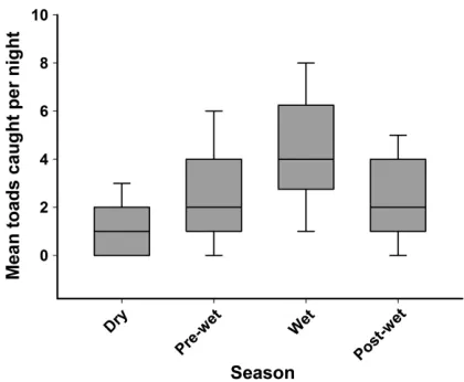
Traps were open for 91 nights in the dry season, 74 nights in the pre-wet season, 54 nights in the wet season, and 39 nights in the post-wet season (total of 516 effective trap nights, given two traps were open each night throughout the trapping period). We trapped 241 toads in the dry season, 387 toads in the pre-wet season, 490 toads in the wet season, and 167 toads in the post-wet season. Toads were most active in the wet season and were least active in the dry season (Fig. 1).

Dry season

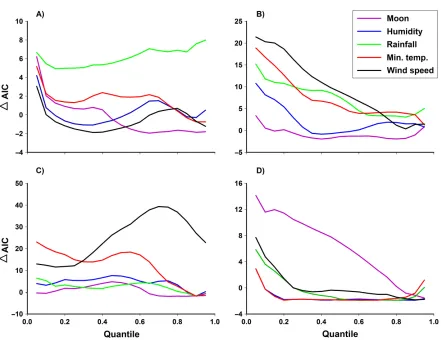
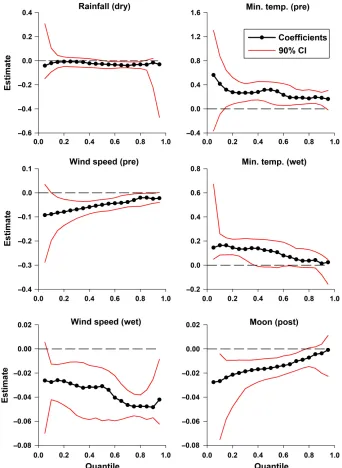
In the dry season, the model including rainfall consistently had the highest average DAIC, across all quantiles (Fig. 2A). We did not include any other variables in a combination model with rainfall, because theDAIC of every other variable was<2 at all quantiles≥0.15 (Fig. 2A). The model that included afirst-order temporal autocorrela-tion effect, in combinaautocorrela-tion with rainfall, was slightly better supported across most of the dis-tribution, but was particularly well supported at lower quantiles (Appendix S2: Fig. S1). In this model, rainfall had a positive effect on all quan-tiles≥0.10 of the toad counts; the estimated par-tial effect was strongest near the minimum of the distribution (Fig. 3). The proportional changes in counts at quantiles ≥0.75 increased 60–67% as

rainfall increased from 20 mm to 33 mm; how-ever, the greatest proportional increases (up to 200%) occurred at quantiles ≤0.25 as rainfall increased from 20 to 33 mm (Fig. 4). This indi-cated that rain events were the strongest driver of activity in the dry season. It may also indicate that generally inactive toads (represented by counts at quantiles≤0.25) were most likely to be trapped during rain events when more than 20 mm fell per night, because the minimum activity (i.e., minimum captures) greatly increased when rainfall was>20 mm.

Pre-wet season

effect, in combination with minimum tempera-ture and wind speed, was well supported, espe-cially at lower quantiles (Appendix S2: Fig. S2). In this model, minimum temperature had a

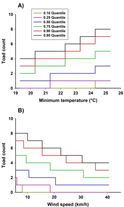
counts were largest (57–200%) at quantiles≥0.50, when the minimum temperature increased from 22°to 26°C. Proportional increases in toad counts when minimum temperature increased from 19° to 22°C were considerably smaller, and only occurred at quantiles ≥0.75. This may indicate that many toads were inactive when the temper-ature was below 22°C; the highest chance of capture for these individuals was when tempera-tures were 22° to 26°C. Conversely, wind speed had a negative effect on all quantiles≥0.10 of the toad counts when minimum temperature was fixed at its median value (Figs. 3, 6B). Propor-tional changes in toad counts were largest when wind speed was below 25 km/h; counts at quan-tiles ≥0.50 decreased 38–67% when wind speed increased from 5 to 25 km/h, and toad counts at quantiles ≤0.25 decreased to zero. The negative effect of wind tapered off when speed exceeded 25 km/h. The combination model suggests that toads are most active in the pre-wet season when the minimum temperature was above 22°C and wind speed was low.

Wet season

In the wet season, minimum temperature and wind speed were the two candidate variable mod-els that had the highest averageDAIC, across all quantiles (Fig. 2C). Minimum temperature was

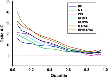
the strongest predictor variable at quantiles≤0.25, while wind speed was the strongest predictor near the middle and upper limits of the distribu-tion. A model including both variables had con-siderable support across all of the distribution, especially at lower limits (Fig. 7). The model that included afirst-order temporal autocorrelation, in combination with minimum temperature and wind speed, was never within 2DAIC units of the selected model at any quantile, and was not con-sidered further. Minimum temperature had a pos-itive effect on all quantiles ≥0.10 of the toad counts, when wind speed wasfixed at its median value; however, this effect was considerably stron-ger at lower quantiles (Fig. 3). The proportional changes in counts increased 67–200% at quantiles ≤0.5 when temperature increased from 24° to 28°C; however, proportional changes in counts at higher quantiles were comparatively lower, across the same temperature range (Fig. 8A). The obvi-ous interpretation is that even the lowest mini-mum temperatures in the wet season were warm enough to allow toad activity, however when tem-peratures were higher, the minimum activity (i.e., minimum captures) greatly increased. Wind Fig. 4. Estimated quantile count model for cane toad

captures (n=182) on Orpheus Island in the dry season (June–August 2013), as a function of rainfall and a

first-order autocorrelation effect, estimated using a ceiling function. An average of estimates form =500 random jitterings for cane toad counts was used.

speed had a negative effect on all quantiles≥0.10 of the toad counts, when minimum temperature was fixed at its median value (Fig. 3). When s≥ 0.75, the proportional changes in counts decreased 42–45% as wind speed increased from 5 to 20 km/h (Fig. 8B). This indicated that wind may have limited toad activity in the wet season, given that the rate of change of toad counts was

highest at quantiles near the maximum of the dis-tribution. Overall, the model indicated that warm, still nights were most conducive to toad activity. While minimum temperatures were generally warm enough to facilitate high toad activity, wind speed constrained the maximum activity of toads, and may be the primary driver of activity in the wet season.

Post-wet season

In the post-wet season, moon luminosity was the strongest predictor of toad activity; the model including moon luminosity had the high-est averageDAIC form= 500 replications of jit-tered toad counts, across most quantiles (Fig. 2D). This model was strongest at the lower limits of the distribution, and gradually weak-ened at higher quantiles. The model that included a first-order temporal autocorrelation, in combination with moon luminosity, was never within 2DAIC units of the selected model at any quantile, and was not considered further. Although the negative effect of moon luminosity on toad activity was strong at quantiles ≤0.50 Fig. 7. Change in averageDAICs of models contain-ing minimum temperature, wind speed, and a combi-nation of both variables, acrosss 2{0.05, 0.10, 0.15, . . ., 0.95}, for m=500 replications of z = y+U[0, 1), on Orpheus Island, in the wet season (December 2013– February 2014). The relative strength of models con-taining individual environmental variables in the wet season is shown in Fig. 2C. In the wet season, a combi-nation model containing minimum temperature and wind speed was strongest at quantiles ≤0.70, and within 2DAIC units of the strongest model at upper quantiles. AIC, Akaike’s information criterion.

Fig. 6. Estimated quantile count model, including a

(Figs. 2D, 3), none of the models had an average DAIC >2 at quantiles≥0.80, indicating that none of the measured variables limited toad activity in the post-wet season. The proportional changes in counts decreased 67–200% (to zero in some cases) at quantiles ≤0.50 as moon luminosity increased from 0% to 52% (Fig. 9). The decrease in proportional changes in counts was not as rapid at moderate to high moon luminosities (≥52%), at quantiles where counts were above

zero. This may indicate that most toads preferred dark conditions in the post-wet season, and were not active when moon luminosity was ≥52%; however, some toads were always active, regard-less of moon luminosity.

D

Overall, several different variables had syner-gistic and antagonistic effects on cane toad activ-ity. Using our combination of statistical techniques, we detected the influence of environ-mental variables on both lower and upper bounds of toad activity. We also found that there was high seasonal variability in cane toad activ-ity; toads were more active in the wet season (December–February) and less active in the dry season (June–August). Furthermore, there was variability in the combinations of environmental variables that influenced toad activity, depend-ing on the time of year. This may be because par-ticular environmental variables were sufficient for minimum activity during certain seasons, but not others.

Results acquired using model selection on quantile count models were consistent with expectations based on the physiological require-ments of cane toads. For example, rainfall was the strongest predictor of toad activity in the dry season, across all measured quantiles. Minimum

Fig. 8. Estimated quantile count model for cane toad captures (n=108) on Orpheus Island in the wet sea-son (December 2013–February 2014), as a function of minimum temperature, with wind speed fixed at its median value (A), and as a function of wind speed, with minimum temperaturefixed at its median value (B), estimated using a ceiling function. An average of estimates form =500 random jitterings for cane toad counts was used.

toad activity increased up to 200% when rainfall exceeded 20 mm, suggesting that many toads may be generally inactive during the dry season, and only emerge from their burrows, forage, or search for mates, when rainfall is high. Cane toads emerge from their burrows more fre-quently (Seebacher and Alford 1999), and move longer distances (Schwarzkopf and Alford 2002) when there is more atmospheric and soil mois-ture, probably because moist conditions limit water lossviatheir permeable skin (Schwarzkopf and Alford 1996). The first-order temporal auto-correlation effect evident in the dry season indi-cated that activity on a given night partially predicted activity on the subsequent night. This could be interpreted as a lagged effect of rainfall, where soil moisture was comparatively high for several consecutive nights after rain, which cre-ated extended periods of favorable conditions for toad activity. Rainfall in the dry season was rare; therefore, the physiological cost of movement was generally high. Toad capture rates increased with rainfall, probably because the cost of move-ment (i.e., water loss) was lower than in dry peri-ods (Schwarzkopf and Alford 2002).

In the wet season, wind speed appeared to limit toad activity (Fig. 8B). This may be because evap-orative water loss rates increase when wind speed is high (Bentley and Yorio 1979); therefore, toads may reduce activity when wind exceeds a certain speed. High winds may also reduce insect activity (Holyoak et al. 1997), so toads may be less active for feeding, and our insect-attracting UV light lure may also be less attractive when it is windy (McGeachie 1989). Windy conditions may have also increased the excess attenuation of the call used to lure toads, and therefore reduced the distance the call carried (Larom et al. 1997). The strongest predictor model in the wet season also included minimum temperature, the effect of which was strongest at lower quantiles. Toad captures increased a great deal (67–200%) at lower quantiles (≤0.5), when minimum temperature increased 4°C (from 24°to 28°C), while captures at upper quantiles, across the same temperature range, remained relatively stable. This large increase in toad captures with a relatively small increase in ambient temperature indicates that minimum temperature in the wet season was well above the minimum threshold for toad activity, because many toads were active, regardless of

temperature. The increase in minimum toad activ-ity is consistent with the strong increase in toad locomotor performance from a preferred tempera-ture of 24°C toward a thermal optimum of approximately 30°C (Kearney et al. 2008). The availability of temperatures conducive to high performance may have encouraged activity from even the most inactive toads, and greatly increased their chance of capture.

Our toad activity models included various com-binations of rainfall, minimum temperature, and wind speed in most seasons. However, in the post-wet season, moon luminosity appeared to influence toad activity, especially at lower quan-tiles. Activity in the post-wet season may occur because there is a need to feed after breeding in the wet season (Yasumiba et al. 2016). Toads strongly avoid light (Davis et al. 2015), but will feed under lighted conditions if there is food available (Gonzalez-Bernal et al. 2011). We sug-gest some toads limited their activity as ambient light increased; however, bolder (or hungrier) individuals may have continued feeding in spite of the moonlight. Several studies report depressed nocturnal activity in amphibians due to moon-light, probably because amphibians avoid moon-light, which may occur because there is an increase in their detectability to predators in lighter condi-tions (reviewed in Grant et al. 2012). It was surprising that the moonlight effects were only detectable in one season and that the magnitude of reduction in activity appeared to vary across the moon luminosity spectrum. Possibly, the effects of moonlight were most detectable in this season because, after the wet season, toad activity was most strongly determined by foraging needs. Temperature and humidity were still high enough to encourage activity, so that an otherwise weak effect of moon luminosity, not detectable in other seasons, when other factors (such as reproduction or hydration) were affecting the toad’s propensity to be active, then became influential.

quantile regression, the interval between 0.10 and 0.90 quantile regression estimated at any specified value of X is an 80% prediction interval for a single future observation of y (Cade and Noon 2003). For example, in the dry season, the 80% prediction interval increases from 0–4 toads when rainfall is 10 mm, to 1–8 toads when rain-fall is 25 mm (Fig. 4). Conversely, in the wet sea-son, the 80% prediction interval decreases from 2–10 toads when wind speed is 10 km/h to 1–5 toads when wind speed is 25 km/h (Fig. 8B). Our quantile count models characterize the vari-ability of prediction intervals for future toad counts reasonably, in each season, with few assumptions. An additional advantage of the quantile count model over traditional parametric count models is that it avoids having to select from among various parametric distributions (e.g., Poisson, negative binomial, and their zero-inflated counterparts).

Examining rates of change at various points across cane toad capture distribution models, using model selection, enabled us to more effec-tively examine the influence of several environ-mental factors across the entire distribution. Our jittered quantile count model is particularly use-ful when the dependent variable includes many tied values, across a small range of values. Indeed, nightly numbers of toads captured often ranged between 0 and 5 (89% of the toad counts fell within this range). Thus, our jittered quantile count model allowed for interpretation of a dis-crete count response variable with many tied val-ues, across an extremely limited range of values (Machado and Santos Silva 2005, Cade and Dong 2008). Finally, our model selection procedure allowed us to select strong predictor models at any quantile in the distribution to include in combination models, while simultaneously rejecting weak predictor models that may have otherwise added an uninformative parameter to the combination model (Arnold 2010). This method streamlined the model selection process and reduced the chance of misinterpretation of AIC results (see Arnold 2010).

Model selection on quantile count models was extremely effective at examining, in depth, the effect of environmental variables on cane toad trapping rates, and activity. Our study provides a simple example of this methodology, using onlyfive environmental variables. Future studies

could incorporate a wider range of variables to better approximate the factors effecting activity, and counts. This methodology could also be used for standard quantile regressions, when the range of values is large, with few tied values, using a process similar to generalized linear modeling to obtain slope estimates at various quantiles across the distribution. The indepen-dent use of AIC model selection, and quantile count models, is not new; however, we have demonstrated that the use of both methods, simultaneously, can allow us to examine exten-sively the relationship between environmental variables and rates of capture in trapping and mark–recapture regimes, and also to determine which of these variables affect the study organ-ism’s activity.

A

We thank O.I.R.S staff for help with data collection and G. Wensor for technical support. Toads were trapped, handled, and euthanized in accordance with James Cook University Animal Ethics Protocols A1838 and A2046. Funding was provided by the Australian Research Council (Linkage Grant LP10020032). Any use of trade,firm, or product names is for descriptive purposes only and does not imply endorsement by the U.S. Government. We have no conflict of interests.

L

C

Akaike, H. 1974. A new look at the statistical model identification. IEEE Transactions on Automatic Control 19:716–723.

Akaike, H. 1998. Information theory and an extension of the maximum likelihood principle. Pages 199–213. in E. Parzen, K. Tanabe, and G. Kitagawa, editors. Selected papers of Hirotugu Akaike. Springer, New York, New York, USA.

Arnold, T. 2010. Uninformative parameters and model selection using Akaike’s information criterion. Jour-nal of Wildlife Management 74:1175–1178.

Bentley, P. J., and T. Yorio. 1979. Evaporative water loss in anuran amphibia: a comparative study. Com-parative Biochemistry and Physiology Part A: Phy-siology, 62:1005–1009.

Burnham, K. P., and D. R. Anderson. 2004. Multimodel inference: understanding AIC and BIC in model selection. Sociological Methods and Research 33:261–304.

Cade, B. S., and B. R. Noon. 2003. A gentle introduc-tion to quantile regression for ecologists. Frontiers in Ecology and the Environment 1:412–420. Cade, B. S., B. R. Noon, and C. H. Flather. 2005.

Quan-tile regression reveals hidden bias and uncertainty in habitat models. Ecology 86:786–800.

Cade, B. S., B. R. Noon, R. D. Scherer, and J. J. Keane. 2017. Logistic quantile regression provides improved estimates for bounded avian counts: a case study of California Spotted Owlfledgling pro-duction. Auk 134:783–801.

Cade, B. S., J. D. Richards, and P. W. Mielke Jr. 2006. Rank score and permutation testing alternatives for regression quantile estimates. Journal of Statis-tical Computation and Simulation 76:331–355. Cade, B. S., J. W. Terrell, and R. L. Schroeder. 1999.

Estimating effects of limiting factors with regres-sion quantiles. Ecology 80:311–323.

Chamaille-Jammes, S., H. Fritz, and F. Murindagomo. 2007. Detecting climate changes of concern in highly variable environments: Quantile regressions reveal that droughts worsen in Hwange National Park, Zimbabwe. Journal of Arid Environments 71:321–326.

Cohen, M. P., and R. A. Alford. 1996. Factors affecting diurnal shelter use by the cane toad,Bufo marinus. Herpetologica 52:172–181.

Davis, J. L., R. A. Alford, and L. Schwarzkopf. 2015. Some lights repel amphibians: implications for improving trap lures for invasive species. Interna-tional Journal of Pest Management 61:305–311. Geraci, M. 2016. Qtools: a collection of models and

tools for quantile inference. R Journal 8(2):117–138. Gibbons, J. W., and D. H. Bennett. 1974. Determination of anuran terrestrial activity patterns by a drift fence method. Copeia 1974:236–243.

Gonzalez-Bernal, E., G. P. Brown, E. Cabrera-Guzman, and R. Shine. 2011. Foraging tactics of an ambush predator: the effects of substrate attri-butes on prey availability and predator feeding success. Behavioral Ecology and Sociobiology 65:1367–1375.

Grant, R., T. Halliday, and E. Chadwick. 2012. Amphibians’response to the lunar synodic cycle— a review of current knowledge, recommendations, and implications for conservation. Behavioral Ecol-ogy 24:53–62.

Henzi, S. P., M. L. Dyson, S. E. Piper, N. E. Passmore, and P. Bishop. 1995. Chorus attendance by male and female painted reed frogsHyperolius marmora-tus: environmental factors and selection pressures. Functional Ecology 9:485–491.

Holyoak, M., V. Jarosik, and I. Novak. 1997. Weather-induced changes in moth activity bias measure-ment of long-term population dynamics from light

trap samples. Entomologia Experimentalis et Applicata 83:329–335.

Huey, R. B. 1982. Temperature, physiology, and the ecology of reptiles. Pages 25–74 in C. Gans and F. H. Pough, editors. Biology of the reptilia. Vol-ume 12. Academic Press, New York, New York, USA.

Huey, R. B., and R. D. Stevenson. 1979. Integrating thermal physiology and ecology of ectotherms: a discussion of approaches. American Zoologist 19:357–366.

Johnson, M. F., S. P. Rice, and I. Reid. 2014. The activity of signal crayfish (Pacifastacus leniusculus) in rela-tion to thermal and hydraulic dynamics of an allu-vial stream, UK. Hydrobiologia 724:41–54.

Kearney, M., B. L. Phillips, C. R. Tracy, K. A. Christian, G. Betts, and W. P. Porter. 2008. Modelling species distributions without using species distributions: the cane toad in Australia under current and future climates. Ecography 31:423–434.

Koenker, R. 1994. Confidence intervals for regression quantiles. Pages 349–359 in P. Mandl and M. Huskova, editors. Asymptotic statistics: proceed-ings of the 5th Prague Symposium. Physica-Verlag, Heidelberg, Germany.

Koenker, R. 2012. Package‘quantreg’. http://cran.r-pro ject.org/web/packages/quantreg/quantreg.pdf Koenker, R., and G. Bassett. 1978. Regression

quan-tiles. Econometrica 46:33–50.

Koenker, R., and J. A. F. Machado. 1999. Goodness of

fit and related inference processes for quantile regression. Journal of the American Statistical Association 94:1296–1310.

Larom, D., M. Garstang, K. Payne, R. Raspet, and M. A. Lindeque. 1997. The influence of surface atmo-spheric conditions on the range and area reached by animal vocalizations. Journal of Experimental Biology 200:421–431.

Lei, J., and D. T. Booth. 2014. Temperature,field activ-ity and post-feeding metabolic response in the Asian house gecko, Hemidactylus frenatus. Journal of Thermal Biology 45:175–180.

Machado, J. A. F., and J. S. Santos Silva. 2005. Quan-tiles for counts. Journal of the American Statistical Association 100:1226–1237.

McGeachie, W. J. 1989. The effects of moonlight illumi-nance, temperature and wind speed on light-trap catches of moths. Bulletin of Entomological Research 79:185–192.

Muller, B. J., D. A. Pike, and L. Schwarzkopf. 2016. Defining the active space of cane toad (Rhinella marina) advertisement calls: Males respond from further than females. Behaviour 153:1951–1969. Muller, B. J., and L. Schwarzkopf. 2017. Success of

characteristics of lures. Pest Management Science. https://doi.org/10.1002/ps.4629

Neter, J., M. H. Kutner, C. J. Nachtsheim, and W. Wasserman. 1996. Applied linear statistical models. Volume 4. Irwin, Chicago, Illinois, USA.

Price, M. V. 1977. Validity of live trapping as a measure of foraging activity of heteromyid rodents. Journal of Mammalogy 58:107–110.

Richards, S. A., M. J. Whittingham, and P. A. Stephens. 2011. Model selection and model averaging in behavioural ecology: the utility of the IT-AIC framework. Behavioural Ecology and Sociobiology 65:77–89.

Rowcliffe, J. M., R. Kays, B. Kranstauber, C. Carbone, and P. A. Jansen. 2014. Quantifying levels of animal activity using camera trap data. Methods in Ecol-ogy and Evolution 5:1170–1179.

Schwarzkopf, L., and R. A. Alford. 1996. Desiccation and shelter-site use in a tropical amphibian: com-paring toads with physical models. Functional Ecology 10:193–200.

Schwarzkopf, L., and R. A. Alford. 2002. Nomadic movements in tropical toads. Oikos 96:492–506. Seebacher, F., and R. A. Alford. 1999. Movement and

microhabitat use of a terrestrial amphibian (Bufo marinus) on a tropical island: seasonal variation and environmental correlates. Journal of Herpetol-ogy 33:208–214.

Symonds, M. R. E., and A. Moussalli. 2010. A brief guide to model selection, multimodel inference and model averaging in behavioural ecology using Akaike’s information criterion. Behavioural Ecol-ogy and SociobiolEcol-ogy 65:13–21.

Terrell, J. W., B. S. Cade, J. Carpenter, and J. M. Thompson. 1996. Modelling stream fish habitat limitations from wedged-shaped patterns of varia-tion in standing stock. Transacvaria-tions of the Ameri-can Fisheries Society 125:104–117.

Tester, J. R., and J. Figala. 1990. Effects of biological and environmental factors on activity rhythms of wild animals. Chronobiology: Its Role in Clinical Medicine, General Biology, and Agriculture 1990:909–919.

Thomson, J. D., G. Weiblen, B. A. Thomson, S. Alfaro, and P. Legendre. 1996. Untangling multiple factors in spatial distributions: lilies, gophers, and rocks. Ecology 77:1698–1715.

Tracy, C. R. 1976. A model of the dynamic exchanges of water and energy between a terrestrial amphib-ian and its environment. Ecological Monographs 46:293–326.

Upham, N. S., and J. C. Hafner. 2013. Do nocturnal rodents in the Great Basin Desert avoid moonlight? Journal of Mammalogy 94:59–72.

Yasumiba, K., R. A. Alford, and L. Schwarzkopf. 2016. Seasonal reproductive cycles of cane toads and their implications for control. Herpetologica 72:288–292.

Yeager, A., J. Commito, A. Wilson, D. Bower, and L. Schwarzkopf. 2014. Sex, light, and sound: Location and combination of multiple attractants affect probability of cane toad (Rhinella marina) capture. Journal of Pest Science 87:323–329.

Yu, K., and R. A. Moyeed. 2001. Bayesian quantile regression. Statistics and Probability Letters 54: 437–447.

S

I