Specific yield for a two-dimensional flow

Specific yield for a two-dimensional flow

Peter Tritscher,

• W. Wayne Read,

2 and Philip Broadbridge

•

Abstract. We investigate the systematic secular spatial variation of specific yield. As a

vehicle for this analysis

we consider

a canonical

unconfined

aquifer consisting

of a porous

1. Introduction

Estimating the storage capacity and sustainable yield of un- confined aquifers is of fundamental concern to inhabitants of arid and semiarid regions. For each aquifer the water flow regime is determined by a complex interaction among the surface and subsurface recharge-discharge distribution, the aquifer boundaries, and the soil characteristics. Central to quantification of available water is the concept of "specific yield." It has been defined as "... the volume of water that an unconfined aquifer releases from storage per unit surface area of aquifer per unit decline in the water table" [Freeze and Cherry, 1979, p. 62]. This is an implicitly local definition, with the specific yield for any chosen column of soil dependent upon, among other things, the local water flow, water table depth, and soil heterogeneity [Stewart, 1962; Gillham, 1984; Everett et al., 1984; Riekerk, 1989; Fetter, 1994]. In practice, however, spatial variation of specific yield has rarely been considered. Where the water table lowers by one unit of depth, the specific yield is the area of the region between the two relevant water content-depth curves, as depicted geometri- cally in Figure 2.23 of Freeze and Cherry [1979]. In one- dimensional zero-flux solutions these curves are identifiable as moisture release curves, but here they are more general water content profiles. In section 3 we find it convenient to further generalize the definition of specific yield to minus the rate of change of water content depth with respect to water table depth. This definition does not depend on the somewhat arbi- trary choice of unit length in a notional "unit decline in the water table," but it would agree with the previous definition if a very small unit of length were used.

•School of Mathematics and Applied Statistics, University of Wol-

longong, Wollongong, New South Wales, Australia.

2Department of Mathematics and Statistics, James Cook University,

Townsville, Queensland, Australia.

Copyright 2000 by the American Geophysical Union.

Paper number 1999WR900333.

0043-1397/00/1999WR900333509.00

The characteristic moisture release curve and the depth to the water table are the most important factors in determining the volume of water held by the aquifer. It is relatively simple to show from one-dimensional studies that the specific yield is moderately dependent upon the rate of water moving through the soil [Childs, 1960; Gardner, 1958]. However, it is not known if a lateral water flow component, which is typical in two- and three-dimensional flows, bears significance upon the local spe- cific yield and hence on the total volume of water available. The answer to this question has now become accessible since we have developed exact series solutions for saturated- unsaturated flow in two dimensions [Tritscher et al., 1998]. In order to investigate the significance of a two-dimensional flow upon the spatial variability of specific yield, we employ a ca- nonical unconfined aquifer consisting of a porous zone whose cross section is a simple long rectangle. The permeable region overlays an impermeable (or nearly impermeable) base and is bounded by vertical impermeable dikes. In this exploratory model, half of the soil surface is subjected to a uniform infil- tration rate, with the remainder of the soil surface discharging by evaporation. This geometry yields a physically meaningful and practical recharge-discharge profile with a manageable number of parameters while retaining the essential character of two-dimensional flow. We specifically investigate the influ- ence of recharge rate, depth to the water table, and aquifer length for a representative soil.

Previously, numerical methods have been required to solve saturated-unsaturated flow problems with complex boundary geometries and highly variable soil conductivities [Bear and Verruijt, 1987; Zaradny, 1993]. However, it is not widely known that in arbitrary, irregularly shaped domains, linear boundary value problems can be solved by separation of variables and by consequent expansions using nonorthogonal bases for function spaces. With some simple precedents in acoustics by Rayleigh [1945] and in saturated flow by Powers et al. [1967], this method was applied by Read and Volker [1993] and Read [1993] to solve Laplace's equation for saturated flow and by Read and Broad- bridge [1996] for the quasi-linear unsaturated flow of Gardner [1958] and Philip [1969].

1394 TRITSCHER ET AL.: QUASI-STEADY SPECIFIC YIELD

steady infiltration-evaporation

/I., , • , , ,_unsaturated zone, • , .

D. '' ' ' ' ' ' ' ' ß ' '

,,.I , ,, ,, ,, '..'..'--__--'.,' ,' ,' ,'/

- ... .-',',' , ,

at•au

ted//

z/ode;-

F--- •E

Figure 1. Schematic diagram of the soil profile and water recharge-discharge zones.

Recently, Tritscher et al. [1998] have used the analytical se- ries method to solve the steady quasi-linear saturated- unsaturated seepage flow problem for porous domains of ir- regular shape. The seepage problem was modeled as a variational problem to determine the position of the saturated- unsaturated interface. A series solution for the integrand of the penalty functional was derived, which in turn allowed a simple direct numerical method to be applied to achieve an optimum location. By some relatively minor modifications to the formulation of the seepage problem, we may derive a series-type solution for our flow domain wherein the phreatic surface no longer intersects the surface seepage face. For pre- scribed-flux boundary conditions the steady solution for water content is unique only after specifying another parameter such as the total water content. This nonuniqueness of the solution enables us to investigate the relationship between the total water content and water table depth, purely from steady state solutions. The specific yield can in fact be uniquely deter- mined, as a function of total water content.

The series approach has several advantages that are useful for our study. In particular, the explicit dependence of the functional on the position of the phreatic surface yields an accurate location for the water table, which is essential to our analysis. The other advantages, as in the seepage flow problem, are that it affords a realistic description of the water distribu- tion in both saturated and unsaturated zones; the formulation is well defined, algorithmic, and reproducible; no spatial dis- cretizations are necessary; and global solution errors are readily estimated from maximum principles.

2. Model Description

A schematic diagram of the soil horizon used in these anal- yses is given in Figure 1. A layer of permeable soil overlays an impervious base material with vertical dikes at the ends AF and CE. The soil surface AC and basement FE are horizontal so that the cross section of the flow region ABCEF is a rect- angle. The flow region has thickness D, and length L ,, which are measured in the vertical and horizontal directions, respec- tively. At the left vertex on the soil surface we fix the origin of a suitable (x,, z,) coordinate system, with z, positive verti- cally downward. The equations for the soil surface and imper- meable base are given by z, = 0 and z, = D,, respectively.

Steady and essentially uniform infiltration occurs along the soil surface AB from x, - 0 to x, = L,/2, while the rest of

the soil surface BC (fromx, = L,/2 tox, = L,) is subject to mostly uniform evaporation. For a small length where the water supply changes from uniform infiltration to uniform evaporation, we fit a sinusoidal curve to smooth the transition. This is introduced to smooth the phreatic surface so that cal- culation time is reduced. At the soil surface the volumetric water flux takes the form

r,0, 0 -< x, -< 0.4L,

r,(x,) = r,o cos(5rrx,/L,),

0.4L, <x, -< 0.6L,

-r,0, 0.6L, <x, -< L,

(l)

When the soil is sufficiently moist, the rate of evaporation is governed by atmospheric conditions. We have assumed that the atmospheric conditions are uniform over the evaporation region and that the atmospheric demand is near to the rate that balances the volume of water supplied by the infiltration region. This is a reasonable approximation until the soil is very near dry and soil-water transport is the rate-determining pro- cess [Philip, 1957; Gardner and Hillel, 1962]. However, for this case the local specific yield is simply near the maximum value. At this point, we introduce dimensionless variables, using the length L, of the region and the saturated hydraulic con- ductivity K,o. The nondimensional lengths and variables sat- isfy the following relationships:

D, r, r,0

D L,

K,0

K,0

(2)

Note that D is the aspect ratio of the porous region.

2.1. Governing Equation

We assume a homogeneous, isotropic aquifer, with a soil that displays negligible hysteresis in the potential energy-water content relationship and that the flow is governed by Darcy's law. Then for steady saturated-unsaturated flow, the flow equa- tion may be expressed as

V. (K(0) VH) = 0, (3)

where K(O) (= K,(O)/K,o) is the dimensionless hydraulic conductivity, H ( = H,/L, ) is the dimensionless total hydrau-

lic head, 0 (x, z) is the volumetric moisture content, and V is the gradient operator [Bear and Ferruijt, 1987].

In saturated-unsaturated flow, K is a highly nonlinear func- tion of volumetric moisture content. Here we assume K is a constant function for the saturated zone and an exponential function of the pressure head h(x, z) (= H + z) for the unsaturated zone:

1, h

>-

-h0

(4)

K = ea(h+ho),

h < -ho'

This yields the familiar quasi-linear approximation of Gardner [1958] and Philip [1969], which has been found to be suitable for a wide variety of soil types [Pullan, 1990]. The constant h o (=h ,o/L ,) is the dimensionless bubbling pressure so that we may incorporate a tension-saturated zone and a is the dimensionless sorptive number, which, in terms of dimensional units, is the ratio of the geometric length scale L, to the

'"E 0.4-

•0.3 -

=02-

0 '

=01-

o

E 0.0-

I I I I

0 I 2 3 4

Iog•o of pressure head (cm)

o •

-1-

-2-

-:3-

-4- -5-

I I I I

0 I 2 3 4

Iog•o of pressure head (cm)

Figure 2. Soil hydraulic properties for silt loam GE3 (from Figure 7 of van Genuchten [1980]). Circles, solid lines, and dashed line indicate observed, van Genuchten relationship, and quasi-linear fit (a, = 0.0100 cm -1,

from Philip [1984]), respectively.

, = œ,,,. (5)

In our derivation of the solution we will consider the less restrictive case where we have a lower boundary and soil sur- face of arbitrary geometry, as this may be achieved with min- imal additional effort. The rectangular domain is a special case of the arbitrary configuration.

The boundary value problem takes on a particularly simple form if we formulate the problem using a dimensionless stream function, ½(x, z), which quantifies the mass flux in the flow domain. We relate the stream function to the total hydraulic head by

00 OH 00 OH

.... g(o) --. (6)

Ox

- K(O) Oz Oz

Ox

There will be no mass flux across the impermeable basement. Consequently, the stream function on this boundary will be a constant, which we choose as zero, without loss of generality. That is,

½(0, z) = ½(x, ft'(x)) = ½(1, z) = 0.

(7)

Here we have

defined

z = fb(x) as the function

specifying

the

depth of the basement.

We assume the soil surface is subject to vertical infiltration and evaporation at a rate which is a relatively general function

r*(x) such

that J'• r*(x) dx = 0. Subsequently,

the stream

function along this boundary is given by

•0

X

½(x, ft(x)) = R(x) = - r*(x) dx, (8)

where z = ft(x) is the function specifying the elevation of the soil surface. For example, our particular case given by (1)

yields ½(x, 0) =

= ro(sin(5wx)/(5w) - 0.4), ro(x- 1),

0_<x_<0.4

0.4 <x -< 0.6.

0.6<x_<l (9)

2.2. A Variational Formulation

Normally, the boundary value problem (3)-(8) would be solved numerically for the potential H without explicit refer- ence to saturated or unsaturated zones. The location of the phreatic surface, h(x, z) = 0, would be obtained by inversion

techniques. However, we use a more direct approach by posing a functional which incorporates the phreatic surface explicitly.

Actually, we define the surface where the pressure head is equal to the bubbling pressure h (x, z) = -h o and then derive the location of the phreatic surface. However, often the bub- bling pressure is small so the tension-saturated zone may be absorbed into the unsaturated zone.

Let us denote the bubbling-pressure surface h(x, z) = -ho

as z = rt(x). We specify the flux boundary condition over the unsaturated soil surface (8) in terms of the functional

F(,l(x)) = [½(x, ft(x)) - R(x)] 2 dx , (10)

and we minimize F subject to the constraint that the total hydraulic head along the bubbling-pressure surface is the neg- ative of the elevation plus the bubbling pressure:

H(x, *l(x)) = -*l(x) - ho. (11)

Since we can construct explicit series solutions for ½(x, z) and H(x, z), it is assumed that ½ and H satisfy all other governing

equations and boundary conditions stated earlier.

As in the seepage problem [Tritscher et al., 1998], the func- tional (10) represents the root-mean-square error in stream function compared with our target value R(x). In our varia- tional problem this functional is to be minimized over the range of allowed trial functions for the bubbling-pressure sur- face z = r/(x). We then solve the variational problem by a direct numerical scheme such as an Euler method or Ritz's method [El'sgol'ts, 1961] after deriving an explicit form for the stream function, ½(x, z).

1396 TRITSCHER ET AL.: QUASI-STEADY SPECIFIC YIELD

E

o•, 10

c 0

._o

• -10

,l• I I I I ' I I

.--

'• 0 5 10 15 20 25

._

length (m)

._o

0.008

• 0.000

o

I

0- 1- 2- 3- 4-

5- ,

I

I

0

I

I

5 I 15 20 25

length (m)

'5, 0.15- ._o

'• 0.10- • 0.05-

o

0.00 - I

0- 1- 2- 3- 4-

5- I

o 5

I I I

length (m)

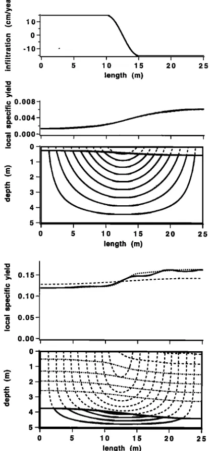
Figure 3. Graphs of the local specific yield for an aquifer

that is almost full or almost empty. Solid, dotted, and dashed

lines indicate actual local specific yield, local specific yield for assumed purely vertical flow, and quasi-static local specific yield, respectively. For comparison we display the infiltration-

evaporation rate and the flow regimes. Shown are normalized streamlines and moisture content contour curves. Dashed curves denote the unsaturated zone. The moisture content

divisions

are 0.0265

cm3/cm

3 units.

The phreatic

surface

is the

{(x, z) ' 0 -< x -< 1 andfb _> z --> r/} and an unsaturated

zoneilu = {(x,z)' 0-<x-< 1 andr/_>z_>f'}.Withthe

above partition, equation (3) yields

V2H = 0

(x, z) 6 ils

(12)

for the governing equation in the saturated zone and yields the steady state Richards' equation

aK

- :0 (x,z)l:u

V. (KVh) •z

in the unsaturated zone. With our assumed exponential rela-

tionship between K and h, the Kirchhoff transformation

h

t• = K dh = K/a (14)

on (13) yields the well-known linear equation

:o

(x z)

Z '

>'0.15

._o

o 0.10

•n 0.05

_o o.oo

' ' ' • ß ' . , ß -• ! - i I •-r---r-,--

0 -]L

...

,...,...•

....

'-,..,_., • , , , ,

/i i i i i i i i i % ... y,. i i• i i i i

/l""r'"r'"r'"r'-'r'-.•.-.•...•. •_ . "i'"'; '-,,•.-.,i,.,•1,..,i, i J

// . ' .... -•-.I,.. j . i i -,,i ...

.=.•,= i ! i ! i i • ... .•., i i • i i i

2 HI' , u'";'"•'-'a.*.-,-.-,.-.,• .... , , ';"-r ... ,.-.r-.. .... /L..,....•...• ,_ , , ,• ß ... ,•.-.-, .... ,...a , •.

J/ , • ;"'c'"'• ... q.-. "" ' • ' ,'"•"r.- r

0 5 10 15 20 25

length (m)

I I I I I

.__.

>'0.15

o0.10

•n 0.05

_.o o.oo

, , , 'j"'i'"i'"t ... "k' .... ß ... } .... •. ... ,. ... ., ... '.:' :r.: ::C'".C" F')"" K'"œ'"•- ... • .... r ... 'r'-q.-.,.-.'.-.'.-.

', • '"•" U' •'"•""•"'• ... •'• .... ß .... •-.-•-.-,.-.•...a...a...

i

i

i

15 ,

215

0 5 10 I 20

length (m)

12

>'0.15

,0

o 0.00

'

2'0 '

4'0 '

'

'

o 10 30 50 60 70

length (m)

Figure 4. Local specific yield for an increase in aquifer depth or an increase in aquifer length. The proportion of soil under infiltration is held constant at 50%. Otherwise, the pictorial

The dimensionless dependent variable/•, commonly referred to as the matric flux potential, is related to the stream function by [Raats, 1970]

Ox

= - •zz + al•

O• = Ox'

(!6)

We specify the boundary conditions across the bubbling- pressure surface dividing the unsaturated and tension- saturated zones. The total hydraulic head must equal the ele- vation plus the bubbling pressure along the bubbling-pressure surface:

H(x, *l(x)) = -*l(x) - ho. (17)

Hence our constraint (11) is satisfied. Additionally, the soil water content tends toward saturation to yield a constant ma- tric flux potential:

/x(x, r•(x))= 1/a. (18)

Finally, we require continuity of stream function:

lim ½(x, z)= lim ½(x, z). (19)

Z-•}- Z-•/+

These boundary conditions with our specification of no flow across the basement (equation (7)) complete the variational formulation. We note that the continuity of stream function

(19) and the continuity of potential (17)-(18) are sufficient to

guarantee continuity of the Darcian flux vector across the bub- bling-pressure surface [Tritscher et al., 1998].

We have transformed the nonlinear boundary value problem (3)-(8) to a form that provides linear governing equations and boundary conditions for each zone of the aquifer. By a Fourier series technique previously applied to Laplace's equation by Read and Volker [1993] and Read [1993] and to quasi-linear flow by Read and Broadbridge [1996], a series form of the solution may be obtained by classical separation of variables. We present an outline of the solution in the appendix. 2.3. Nonuniqueness of the Phreatic Surface

Calculations have shown that for each specific boundary value problem a family of phreatic surfaces exist, each with its own stream function solution. We find that there is sufficient freedom in the solution to allow one point on the phreatic surface to be specified. Alternatively, we may specify the total water content, which, because of our assumed nonhysteretic soil, is in a one-to-one correspondence with the location of the phreatic surface. This may be compared with purely uns•itur- ated flow, wherein the matric flux potential is not uniquely determined and that infinitely many completely unsaturated moisture distributions exist [Read and Broadbridge, 1996]. Analogous to the case of saturated-unsaturated flow, addi- tional specification of the moisture content at one point in the domain is sufficient to guarantee uniqueness [Read and Broad- bridge, 1996]. This nonuniqueness permits a quasi-steady flow to be used for the analysis of specific yield for two-dimensional flow. For fixed and balanced flux boundary conditions we may compare the change in water table depth with the change in the total water content as the solution changes from one steady state to another.

3. Application

We give a detailed analysis for a medium texture soil since this will give a fair indication of the degree of dependence of

• -100-1,.

.-- i i i

•- 0 5 10 15

._

length (m)

>' 0.12

.•_

'• 0.08

_ 0.04

_.o o.oo

'

2•5

20

i i i i

0 'q•--!-4-:,.• _{/I ! % % \ •'-••} ', ', ', ... _{',. ..• '-,•, _ '"/"-.•,.,.&,, m ".•"3'"} ,'"'-4";'": ... i. ... ,-"

E 11 \ \ ' , ,'"', ... : ...

*'• 2 ' ''' ' ; ;

'o 4

0 5 10 15 20 25

length (m)

._e >' 0.12

._•

o 0.08

• 0.04 ...

-

i

_o 0.00

,

•

,

•

0 - ..-,-.-, _{• • • • • • , "'•'-,,•,,..} ... .,...•.-.m...•..- ß - .... .. '-.-.-;g--,- _{",-•,... ' .... •,-.,l,-.• ...} ... _{T. ...}

. . ,, ß , ß ,,-:::.';.-; .... ::::::::::::::::::::::::::

e 8

12

,

•

•

•5

•

215

0 5 10 I 2o

length (m)

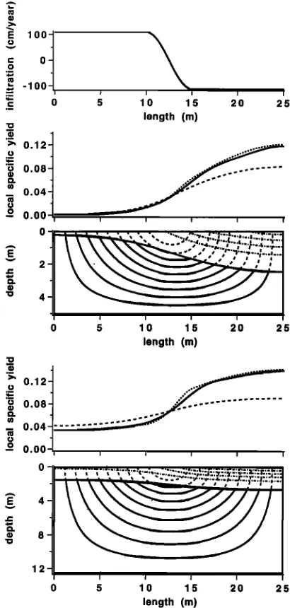
Figure 5. Graphs of local specific yield for an increase in the infiltration rate. Shown are local specific yield for the cases where the aquifer dimensions are the same as in Figure 3 and for a case when the aquifer depth is greater. Otherwise, the pictorial representation is the same as in Figure 3.

specific yield on the aquifer geometry and on recharge condi- tions. Heuristically, the extreme ends of the range of soil types will yield relatively simple results. For sandy soils the band where the soil moisture content is highly varying is relatively narrow, and typically the soil surface is dry. The specific yield in this case becomes essentially that for a deep water table and hence assumes a value near the maximum, regardless of the flow regime. Conversely, an extremely fine clay can support only very low recharge rates before becoming completely sat- urated. Hence, in most recharge situations the aquifer is prac- tically full and the specific yield must be near zero.

For our medium soil we choose a silt loam (GE3) from Reisenauer [1963]. This is chosen because the saturated con- ductivity is approximately in the middle range at 4.96 cm/d.

Additionally, the assumed conductivity function (4) yields a

1398 TRITSCHER ET AL.: QUASI-STEADY SPECIFIC YIELD

0.16-

= 0.14-

>'0.12-

0.10-

0.08 -

.o 0.06-

0.04 -

0.02 -

0.00 -

I

2 3 4 5 6

mean phreatic depth (m)

Figure 6. The regional specific yield for various aquifer dimensions and infiltration rates related to mean phreatic depth. For comparison, the dash-dotted curve is the yield obtained by assuming the water is static and the phreatic surface is horizontal. Symbols are translated as follows: plus signs, r, o = 15 cm/yr, D, = 2.5 m,L, = 25 m; solid circles, r, o - 15 cm/yr, D, - 5 m,L, = 25 m; squares, r, o = 15 cm/yr, D, = 12.5 m, L, = 25 m; triangles, r,o - 15 cm/yr, D, = 5 m, L, = 75 m; solid diamonds, r,o - 110 cm/yr, D, = 5 m,L, = 12.5 m; open diamonds, r,o = 110 cm/yr, D, - 5 m,L, = 25 m; and open circles, r, o = 110 cm/yr, D, = 12.5 m, L, = 25 m.

moisture content and hydraulic conductivity, with our quasi- linear fit, are shown in Figure 2.

Because of the nonuniqueness of the solution for the water content, we are free to specify the depth •(x) of the water table at one location, for example, at x - 0, within some allowable range of values. The boundary conditions and flow equations will then uniquely determine the water content 0 (x, z) and the depth of the phreatic surface •(x) at all other

locations. At a given value x of the horizontal coordinate, the total water volume per unit cross-sectional area is

i,(x) = O(x,, z,) dz, .

Notionally, the specific yield is regarded as the depth of water (- Ai, ) removed from a soil when the water table lowers by a unit length AT,. However, the choice of length unit is some- what arbitrary. A natural unambiguous definition of local di- mensionless specific yield is the limit of (- Ai, )/A •,,

di, di

SY(x)

= d•q, d•q

where • - •,a, and i = i,a,. In practice, we need to evaluate this derivative numerically by comparing the approx- imate phreatic surface locations in different solutions. These numerical evaluations have some errors, and this, along with the small errors in water table location, may explain the small ripples evident in the function SY(x) of Figures 3 and 4.

Figure 3 shows the specific yield for a water table that is just under the soil surface when the aquifer is almost full, and separately for a water table that is near the basement when the aquifer is almost empty. We compare these yields with those predicted by simpler models in order to gauge the effect of any lateral component of water flow. The simplest model is to assume that the water in the column above the phreatic surface is static. This is equivalent to neglecting variations in pressure distribution due to water movement, and the local specific yield is obtainable directly from the moisture release curve. This is a globally one-dimensional model with uniform zero water flux, being the average of the flux at the surface of the two- dimensional region. With this simplification the relative error from the actual specific yield is less than 13%. The error tends to increase as the water table falls. To avoid any ambiguity, we comment that in this model and in any other simpler model, we still calculate the position of the phreatic surface by the full saturated-unsaturated flow model; it is only in the specific yield calculation that we make simplifying approximations.

dimensional flow is not far from the local distribution for purely vertical flow, a situation that seems reasonable, since to raise water against gravity typically requires a greater pressure difference than is needed to move the water horizontally.

In Figure 4 we show the effect of increasing the aquifer depth or increasing the aquifer length. Increasing the depth of the aquifer tends to flatten the water table, and the graph of the specific yield shows this effect. However, an increase in the aquifer length causes a larger variation in the depth to the water table, and we have a corresponding change in the local specific yield curve. Our simpler models still provide good estimates of the actual local specific yield. We comment that one-dimensional studies have shown that for any prescribed evaporation rate there is a maximum depth of the water table after which that rate of evaporation can no longer be main- tained [Gardner, 1958; Philip, 1969]. Physically, the conductiv- ity rate near the surface becomes so low that no amount of suction can drive the water at the requested flow rate. In our formulation we have assumed a constant evaporation rate to simplify the problem. Hence there is a maximum depth for which our solution is valid. For example, the phreatic surface presented for the deep aquifer of Figure 4 is near the maxi- mum depth beyond which our formulation is no longer valid. Finally, we increase the infiltration rate. Figure 5 shows graphs of local specific yield for the same aquifer dimensions as in Figure 3 or for the deep aquifer of Figure 4. The infiltration rate is increased to near the maximum that can be sustained for a valid solution, with the restriction that the phreatic does not intersect the soil surface. In each case the actual local specific yield is approximated well by the simpler model that assumes purely vertical flow. However, the model which neglects the infiltration rate is substantially in error, the relative error being as high as 35%.

For two-dimensional flow we have shown that locally the specific yield may be strongly influenced by the water table depth and mildly dependent on the infiltration rate if the infiltration rate is high. However, it can be reasoned that be- yond some very great depth, further changes in water table depth would cease to have any appreciable effect on the spe- cific yield. For the simple geometry considered, a lateral com- ponent of flow has been found to have an insignificant effect on the local specific yield, and the model that assumes locally purely vertical flow adequately estimates the specific yield.

Although local specific yield gives an indication of the move- ment of the local water table as water is removed or added, the overall specific yield of the aquifer remains to be determined. To address this, let us define the volume of water released per unit decline in the mean water table depth divided by the area of the aquifer as a rudimentary measure of the overall specific yield of the aquifer, and let us label this as the regional specific yield. The division by the aquifer area provides a nondimen- sional unit and allows a comparison among aquifers of differ- ing area.

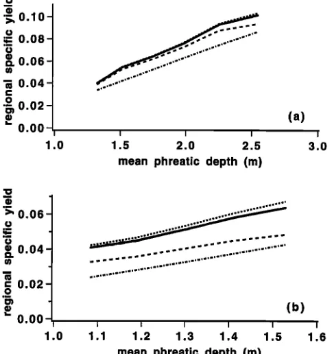
Figure 6 shows the regional specific yield for various aquifer dimensions and infiltration rates as the mean phreatic depth is lowered. We compare these to the yield obtained by assuming the water to be static and the phreatic surface to be horizontal. For most infiltration rates and aquifer dimensions this simple model gives a surprisingly good estimate of the regional spe- cific yield. It is only when there is a large variation in the water table depth that the error may be unacceptable. This occurs for high infiltration rates or long thin aquifers. In Figure 7 we take the flow regimes that have the most deviation from the static

ß •, 0.10-

= 0.08-

n e 0.06-

ß ; 0.04-

o

ß • o.o2-

o.oo - 1.o

(a)

I I I I

1.5 2.0 2.5 3.0

mean phreatic depth (m)

>'0.06

•004

Q. ß

• 0.02

0.00

(b)

I I I I I I

1.0 1.1 1.2 1.3 1.4 1.5 1.6

mean phreatic depth (m)

Figure 7. A comparison of regional specific yield with sim- pler models. Solid, dotted, dashed, and dash-dotted lines de- note actual regional specific yield; yield calculated from as- sumed purely vertical flow; yield calculated from quasi-static local specific yield; and yield obtained with no water flow, the water is assumed static, and the phreatic is horizontal, respec- tively. For our comparison we use aquifer conditions for which the static model was approaching inadequacy: (a) r, o = 15 cm/yr, D, = 5 m, L, = 75 m (see Figure 4 lowermost aquifer

for an example flow regime) and (b) r,o = 110 cm/yr, D, =

5 m, L, = 25 m (see Figure 5 upper aquifer for an example flow regime).

model and compare these with more sophisticated models, namely, the yield calculated from assumed purely one- dimensional vertical flow and the yield calculated from quasi- static local specific yield. The regional specific yield obtained from the assumed purely vertical flow model gives excellent results. The next closest is the yield calculated from quasi-static local specific yield. However, the yield calculated from quasi- static local specific yield may not be much of an improvement over the simple static model.

1400 TRITSCHER ET AL.: QUASI-STEADY SPECIFIC YIELD

• o.12

'.'E 0.08

m 0.04

o

o 0.00

I I I I

I I I I I

0 5 10 15 20 25

length (m)

% 0.08-

,•,

• 0.06-

o

•'0 04-

m ß

c 0.02-

0

ø•0 00-

• ß

1.0

I

•2

.

•6

•

1. I 4 1. 1.8

mean phreatic depth (m)

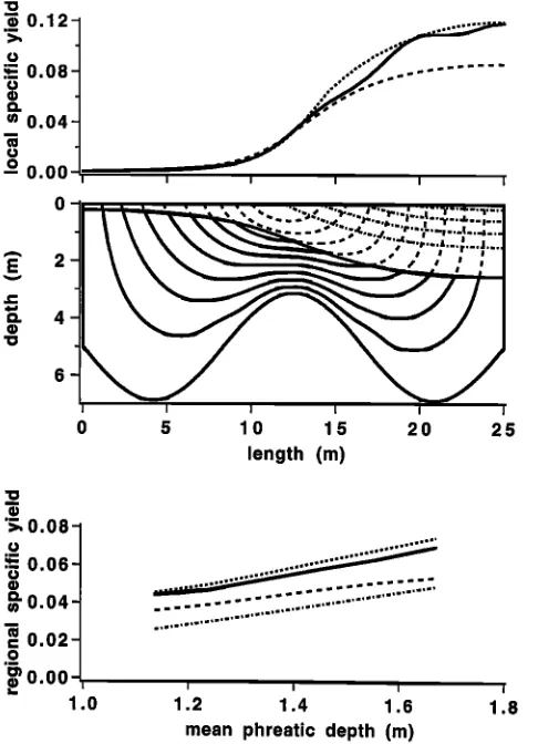
Figure 8. Local specific yield, flow regime, and regional spe- cific yield for an aquifer geometry that yields a more compli- cated unsaturated-zone flow pattern than the simple canonical geometry. The chosen basement geometry forces some of the flow under the evaporating surface to be downward. The leg- end for the local specific yield and flow regime is the same as in Figure 3. The legend for the regional specific yield is the same as in Figure 7. The infiltration parameter r. o is 95 cm/yr.

face where evaporation is occurring. However, this effect is barely significant even when compared with possible errors in the specific yield calculation. We conclude that we have not yet found a flow regime for which the assumed purely vertical flow model is not satisfactory as a good estimator of the specific yield.

4. Conclusions

For two-dimensional flow we have demonstrated that locally the specific yield may be strongly influenced by the water table depth and mildly dependent on the recharge rate if that rate is high. For the simple geometry considered, a lateral component of flow has been found to have an insignificant effect on the local specific yield. For a homogeneous soil a model that as- sumes locally purely vertical flow is more than adequate as an estimator for the specific yield. Perhaps a more important influence on specific yield would be soil heterogeneity. This influence may be investigated in the future by techniques sim- ilar to those employed here.

For the overall yield of an aquifer we find that the simplest model, where the flow through the soil is neglected, i.e., where

the water is static and the phreatic surface is horizontal, gives a reasonable indication of the actual specific yield for most infiltration rates and aquifer dimensions. However, if the in- filtration rate is high or the aquifer is particularly long, then the yield obtained from an assumed purely vertical flow, presup- posing that the phreatic depth is accurately known, gives an excellent estimate of the actual specific yield.

In our formulation we have employed a boundary condition of constant evaporation rate. This in turn has placed a restric- tion on the allowable depth of the phreatic surface, and hence our specific yield covers most of the range possible but falls short of the theoretical maximum. It is suggested for future work that a more realistic radiation-type boundary condition for evaporation at the soil surface be incorporated into the solution. This would ease the restriction on the depth of the phreatic surface, which would broaden the specific yield range available.

Appendix

We present here a series solution for the stream and poten- tial functions. The procedure for the derivation is identical to that of Tritscher et al. [1998]. The solution for the stream and potential may be presented as

• [-A n sinh(n

rrz) + B n cosh(n

,rz)]

x sin (nrrx)/cosh (nrrD) (x, z) • Ils q,(x, z) =

e •z/2

• [ -Cn sinh

(y,z) + D n cosh

(ynZ)

]

x sin (nrrx)/cosh (ynD), (x, z) • Iln

H(x,

z)

-- Aø

- n•l

[An

cosD

(g/qTZ)

--

B

n

sinh

(n

,rz)]

x cos (nrrx)/cosh (nrrD) (x, z) • Ils In (a•)/a - h0 - z (x, z) • Iln,

(A2) where

I•(X, z) = Co

eø•- e ø•/2

• (l/n,r)[(aCn/2

- 'YnDn)

n=l

ß sinh (7,z) + (7•Cn- aDn/2) cosh ('¾nZ)]

ß cos (nrrx)/cosh (7nD), (A3)

with

•n--- •a2/4 + n 2*r2,

(A4)

and An, Bn, Cn, D n are the solution of the following system of linear equations. The coefficients for the saturated zone are given by

j=l

i nt- An -- -kn •, (AS)

A 0 ko

• + • •

n=l i=1

Bn-- E k;7qtAi

,

(m7)

i=1

where

k• h, k•?*, and

kn

• are

(constant)

expansion

coefficients.

These are given by the following relations:

sinh (n •rf b) sin (n •rx)/cosh (n •rD)

= • kjn

•q'

cosh

(i •rf

b) sin

(i •rx)/cosh

(i •rD),

(A8)

i=1

sinh (n•r,1) cos (n•'x)/cosh (n•'D)

=k[n

ah

"}-

E kJff

h

cosh

(i •"1)

cos

(i •'x)/cosh

(i •'D),

i=1

-*l(x) - h0 = k•

(A9)

+ • kn•cosh

(n•'*l)

cos(n'n'x)/cosh

(n'n'D).

n=l

(A10)

The coefficients for the unsaturated zone are given by

-k• - E knq'k;na•Tn/(rt

qr)

n=l

sinh (TnT}) COS (n•'x)/cosh (Tn D)

= k•n

a• + E kiu?

cosh

(Ti'l])

COS

(i•'x)/cosh

(TnD),

i=1

(A16)

e "'v2=

k• + • kn'•cosh(Tnrl)

cos(n'n'x)/cosh(TnD),

(A17)

n=l

e-•'V2/ot

= k• + • k2 cosh

(TnT})

COS

(n•'x)/cosh

(TnD).

n=l

(A18)

Kirkham and Powers [1972] or Read [1993] detail Gram- Schmidt orthogonalization, and Read [1993] details least squares methods to calculate the expansion coefficients.

To provide reproducibility of the figures, we detail the nu- merical implementation for the solutions. As given by Tritscher et al. [1998], we minimize an alternative functional to reduce errors from series truncation, as it is possible that the phreatic is so chosen that the functional (10) is minimized at the ex- pense of the boundary errors. We avoid this problem by incor- porating the boundary errors explicitly, namely,

F(•(x)) = F(•(x)) + Wl•l(•(x)) -I'- W2•2(•(X))

-I- W3•3(T}(X)) -I- W4•4(T}(X)), (A19)

)

= -k•Co + E E k•q'k•?Ti/(i'n')

+ k•na•øZn/(2n'rr)

Cn,

n=l i=1

(All)

-k; + kn*a/(2n•r)

- • kiq'kn•Ti/(iqr

)

i=1

where ei(•q(x)) are root-mean-square (rms) boundary errors:

{ •0L }1/2

•:1

-- L-1

[½(X,

fa)]2 dx ,

(A20)

•:2 = L-1

[H(x, ,r}) -- •]2 dX ,

(A21)

--

'•'ji "nj r•. (j'n') C,

i=1 j=l

-- kn•Co- TnCn/(t't'rt ) (A12)

Dn = kn•

'•- E k;7

•Ci,

(A13)

i=1

with the expansion coefficients kTn •q', kn*, .av. kin , kn •, and kn ,•

given by

sinh (TnT}) sin (n•'x)/cosh (Tn D)

= • kTn

•q'

cosh

(TIT) sin

(i'n'x)/cosh

(%D),

(A14)

i=1

lim e-'•'v2½(x, z)

z-->*l-

= • k• cosh

(TnT})

sin

(n•'x)/cosh

(TnD),

(A15)

n=l

L

e3 = {(L - s(T}))

-1

[lim ½(x, z) - lim ½(x, Z)] 2 dx}

1/2,

(.1) z--->•- z--->• +

(A22)

•4 = (m - S(T}))

-1

[#,(X, '1) -- 1/C•]

2 dx

,

(A23)

and w i are weights.

We choose

2 for the weights

W

i and cal-

culate the expansion coefficients required in the series solution procedure by a least squares method [Read, 1993]. We mini- mize the new functional by Ritz's method [El'sgol'ts, 1961] with cubic splines for the basis functions, and we adjust the knot points by a Nelder-Mead [1965] minimization scheme. Five equally spaced spline segments were chosen for the nodes of the phreatic surface. We specified 10 series terms each in the saturated and unsaturated zones, except for Figure 8, where 20 series terms for the saturated zone were used. Our specific yields were calculated by fourth-order finite differences. The abscissae spacing in the finite differences were from 0.0025 to 0.01 nondimensional units. In dimensional units this corre- sponds to a difference in the water table depth by approxi-

1

1402 TRITSCHER ET AL.: QUASI-STEADY SPECIFIC YIELD

Acknowledgments. We thank J. H. Knight for helpful comments

and the anonymous referees for constructive criticisms. We also grate-

fully acknowledge the financial support provided by the Australian

Research Council, Department of Employment, Education, Training

and Youth Affairs, Canberra, Australia.

References

Bear, J., and A. Verruijt, Modeling Groundwater Flow and Pollution, D.

Reidel, Norwell, Mass., 1987.

Childs, E. C., The nonsteady state of the water table in drained land,

J. Geophys. Res., 65, 780-782, 1960.

El'sgol'ts, L. E., Calculus of Variations, Pergamon, Tarrytown, N.Y.,

1961.

Everett, L. G., L. G. Wilson, and E. W. Hoylman, Vadose Zone Mon-

itoring for Hazardous Waste Sites, Noyes Data Corp., Park Ridge,

N.J., 1984.

Fetter, C. W., Applied Hydrogeology, p. 376, Prentice-Hall, Englewood

Cliffs, N.J., 1994.

Freeze, R. A., and J. A. Cherry, Groundwater, Prentice-Hall, Engle-

wood Cliffs, N.J., 1979.

Gardner, W. R., Some steady state solutions of the unsaturated mois-

ture flow equation with application to evaporation from a water table, Soil Sci., 85, 228-232, 1958.

Gardner, W. R., and D. I. Hillel, The relation of external evaporative

conditions to the drying of soils, J. Geophys. Res., 67, 4319-4325,

1962.

Gillham, R. W., The capillary fringe and its effect on the water-table

response, J. Hydrol., 67, 307-324, 1984.

Kirkham, D., and W. L. Powers, Advanced Soil Physics, Wiley-

Interscience, New York, 1972.

Nelder, J. A., and R. Mead, A simplex method for function minimi- zation, Comput. J., 7, 308-313, 1965.

Philip, J. R., Evaporation, and moisture and heat fields in the soil, J.

Meteorol., 14, 354-366, 1957.

Philip, J. R., Theory of infiltration, Adv. Hydrosci., 5, 215-296, 1969.

Philip, J. R., Nonuniform leaching from nonuniform steady infiltration,

Soil Sci. Soc. Am. J., 48, 740-749, 1984.

Powers, W. L., D. Kirkham, and G. Snowden, Orthonormal function

tables and the seepage of steady rain through soil bedding, J. Geo-

phys. Res., 72, 6225-6237, 1967.

Pullan, A. J., The quasi-linear approximation for unsaturated porous

media flow, Water Resour. Res., 26, 1219-1234, 1990.

Raats, P. A. C., Steady infiltration from line sources and furrows, Soil

Sci. Soc. Am. Proc., 34, 709-714, 1970.

Rayleigh, Lord (J. W. Strutt), The Theory of Sound, 2nd ed., Dover,

Mineola, N.Y., 1945.

Read, W. W., Series solutions for Laplace's equation with nonhomo-

geneous mixed boundary conditions and irregular boundaries, Math.

Comput. Modell., 17, 9-19, 1993.

Read, W. W., and P. Broadbridge, Series solutions for steady unsat-

urated flow in irregular porous domains, Transp. Porous Media, 22,

195-214, 1996.

Read, W. W., and R. E. Volker, Series solutions for steady seepage

through hillsides with arbitrary flow boundaries, Water Resour. Res.,

29, 2871-2880, 1993.

Reisenauer, A. E., Methods for solving problems of multidimensional,

partially saturated steady flow in soils, J. Geophys. Res., 68, 5725-

5733, 1963.

Riekerk, H., Influence of silvicultural practices on the hydrology of

pine flatwoods in Florida, Water Resour. Res., 25, 713-719, 1989.

Stewart, J. W., Water-yielding potential of weathered crystalline rocks

at the Georgia Nuclear Laboratory, in Geological Survey Research,

U.S. Geological Survey professional paper, B106-B107, 1962.

Tritscher, P., W. W. Read, P. Broadbridge, and J. H. Knight, Steady

saturated-unsaturated flow in irregular porous domains, Preprint

4/98, School of Math. and Appl. Stat., Michael Birt Libr., Univ. of

Wollongong, Wollongong, N.S.W., Australia, 1998.

Van Genuchten, M. T., A closed-form equation for predicting the

hydraulic conductivity of unsaturated soils, Soil Sci. Soc. Am. J., 44,

892-898, 1980.

Zaradny, H., Groundwater Flow in Saturated and Unsaturated Soil,

A. A. Bolkema, Rotterdam, Netherlands, 1993.

P. Broadbridge and P. Tritscher, School of Mathematics and Ap-

plied Statistics, University of Wollongong, N.S.W. 2522, Australia.

([email protected]; [email protected]) W. W. Read, Department of Mathematics and Statistics, James

Cook University, Townsville, Queensland 4811, Australia.

([email protected])