Interference cancellation assisted lattice reduction aided detection for MIMO systems

Interference cancellation assisted lattice-reduction aided

detection for MIMO systems

Kyungchun Lee1, Joohwan Chun1, and Lajos Hanzo2 1_{Dept. of EECS, KAIST}

373-1 Guseong-dong, Yuseong-gu, Daejeon 305-701, Republic of Korea e-mail: [email protected]; [email protected]

2_{School of ECS, Univ. of Southampton, SO17 1BJ, UK} e-mail: [email protected]

Abstract— In this paper, we proposed and investigated the optimal successive interference cancellation (SIC) strategy designed for lattice-reduction aided multiple-input multiple-output (MIMO) detectors. For the sake of generating the optimal MIMO symbol estimate at each SIC detection stage, we model the so-called effective symbols generated with the aid of lattice-reduction as joint Gaussian distributed random variables. However, after lattice-reduction, the effective symbols become correlated and exhibit a non-zero mean. Hence, we derive the optimal minimum-mean-squared-error (MMSE) SIC detector, which updates the mean and variance of the effective symbols at each SIC detection stage. As a result, the proposed detector achieves an approximately 3 dBE_b/N₀ gain and performs close to the maximum likelihood detector.

I. INTRODUCTION

The computational complexity of the maximum likelihood (ML) MIMO detector increases exponentially with the number of transmit antennas [1]. The family of reduced-complexity detection algorithms may be classified as linear and nonlinear detectors [2]. Although linear detectors, such as the linear minimum-mean-squared-error (MMSE) detector, typically exhibit a low complexity, their perfor-mance is significantly worse than that of the ML detector. The non-linear successive interference cancellation (SIC) algorithm detects each symbol sequentially with the aid of classic redemodulation and subtraction based canceling operations, and exhibits an attrac-tive performance versus complexity trade-off [2]–[4]. However, its performance is nonetheless inferior with respect to ML detection [4]. The family of lattice-reduction (LR) aided algorithms [5]–[7] transforms the MIMO channel encountered into an effective channel matrix, which is near-orthogonal. Therefore, suboptimal detectors combined with LR become capable of attaining full diversity and hence achieve a performance close to that of the ML detector.

Following the LR operation, the resultant symbols are no longer mutually independent and hence they exhibit non-zero cross-correlations, which are determined by the specific LR transformation matrix used. Furthermore, since the resultant effective symbols are correlated, their mean and covariance should be updated after the symbol detection operation of each spatial detection layer. Although numerous studies of LR-aided SIC detectors have been published [5]–[7], no conclusive proposals have been made for handling their non-zero means and the correlation of the symbol.

Hence, in this paper, we derive the optimal LR-aided SIC detector, which is capable of adequately handling the non-zero mean as well as correlation of the effective symbols. We assume that the effective symbols are Gaussian distributed random variables with

This work was supported in part by ADD through a grant managed by RDRC, and by KOSEF under contract R01-2003-000-10829-0 as well as a grant managed by MICROS ERC. Furthermore, the financial support of the EPSRC, UK and that of the European Union under the auspices of the Newcom and Phoenix projects is gratefully acknowledged.

non-zero means as well as covariances, and perform the optimum inter-antenna interference cancellation operation at each detection stage, where the optimization is carried out in the MMSE sense. This paper is organized as follows. Section II describes the signal model and the LR-aided detection. In Section III, the optimal MMSE-SIC algorithm invoked in the context of LR-aided detection is presented. Section VI provides our simulation results, while Section V offers our conclusions.

II. SYSTEMMODEL

A. Signal Model

We consider Nt transmit antennas andNr receive antennas. The channel is assumed to be frequency-flat fading and its time-domain variation is deemed negligible over a transmission frame duration. The overall channel can be represented by an(Nr×Nt)-dimensional complex-valued matrix

H=

2 6 6 6 4

h11 · · · h1Nt h21 · · · h2Nt

..

. . .. ...

hNr1 · · · hNrNt

3 7 7 7

5, (1)

wherehmnis the complex-valued non-dispersive fading coefficient of the channel between thenth transmit and themth receive antenna. The signal encountered at themth receive antenna is formulated as

ym=

P_Nt

n=1hmnxn+vm , wherexnis the symbol transmitted from the nth antenna, andvm is the zero-mean complex Gaussian noise having a variance of σv2 per dimension. In this paper, we assume thatxn represents quadrature amplitude modulated (QAM) signals. The overall received signals can be represented asy=Hx+v, where we havey= [y1 y2 · · · yNr]T,x= [x1 x2 · · · xNt]T and v_{= [v}

1 v2 · · · vNr]T, while(·)T represents the matrix transpose.

For later notational convenience, we introduce an equiva-lent real-valued expression y = Hx + v, where we have x = [Re(x₎T _Im(x)T_]T_{, y = [Re(y)}T _Im(y)T_]T_{, v =}

[Re(v₎T _Im(v)T_]T _and H=

»

Re(H_{) −Im(H)}

Im(H_{) Re(H)} –

. (2)

We set the dimension ofHto(M×N), whereM= 2Nr,N= 2Nt.

B. LR-aided Detection

having unity elements. For example, when the elements ofxassume values of {−3/√5,−1/√5,1/√5,3/√5} in the 16-QAM phasor contellation,dbecomes2/√5and the elements ofx˜belong to the decision interval 1 of the phasor points of{−1,0,1,2}.

Given the integer-valued transmitted symbolx˜, the received signal of y = Hx+v is rewritten as y˜ = ˜Hx˜+v, where we have

˜

y=y+dH1N/2andH˜ =dH.

Following the scaling and shifting operations of˜x=x/d+1N/2, according to the LR principles, we transform the channel matrix H˜ with the aid of T and T−1 having integer elements yielding the effective received signal model

˜

y= ˜HTT−1_{x˜+v=Gs+v, (3)} where we introduced the effective symbols of

s=T−1_{x˜ (4)}

andG= ˜HT. SinceT−1 andx˜are composed of integer elements, the effective symbol vectorsalso has integer elements. After detect-ing the effective symbols of s = T−1˜x, we can further transform them tox usingx˜ =Ts and x˜ =x/d+1N/2. According to (3) in LR-aided detection, the channel matrixH˜ =dHis rotated using the matrix Tand this operation is designed to render the effective channel matrixG= ˜HT‘as orthogonal as possible’. This operation guarantees that despite using sub-optimal detectors, we are capable of approaching the ML detector’s performance.

For example, when we have

˜

H=

2 6 6 4

0.8 0.04 −0.02 −2.3 −2.3 −0.1 0.7 4.2

0.02 2.3 0.8 0.04 −0.7 −4.2 −2.3 −0.1

3 7 7

5, (5)

we can setTandT−1 to

T=

2 6 6 4

1 0 2 −2

−1 1 0 0 2 −2−1 0 0 0 1 −1

3 7 7 5,T−1=

2 6 6 4

1 0 0 −2 1 1 0 −2 0−2 −1 0 0−2 −1−1

3 7 7 5. (6)

As an indicator of orthogonality of a matrix, we use the condition number, which is defined as the ratio of the maximum singular value and the minimum singular value of a matrix. As the condition number get closer to 1, the matrix becomes orthogonal. The condition numbers of H˜ and G = ˜HT are 11.8 and 1.7, respectively. By multiplyingTtoH˜, the condition number is considerably reduced, which implies that G causes much smaller errors than H˜ in the suboptimal detectors.

Several algorithms have been proposed for generating the matrix T [8]–[10]. The Lenstra, Lenstra and Lovasz (LLL) algorithm [8] constitutes a popular approach, which has a complexity that increases at a polynomial order as a function of the number Nt of transmit antennas. Hence, we invoke the the LLL lattice-reduction algorithm in the context of MIMO detection.

Let us consider two basis vectors {b1, b2} in a lattice. To minimize the correlation between two vectors, we perform the orthogonalization :

b₂=b₂−μ2,1b1, (7) whereμj,k is defined asμj,k =|bTjbk|/bk2. Whenμ2,1 is not an integer, (7) can change the lattice. Therefore, we modify (7) to

b₂=b₂− μ2,1b1, (8) where · denotes the operation rounding a number to the nearest integer. For the further reduction of the correlation, we check the

TABLE I

THELLLALGORITHM

Input:BI= [b1, b2, · · ·, bN], 1/4< δ <1 n= 2

whilen≤N

for l=n−1, n−2,· · ·, 1

bn=bn− μn,lbl % size-reduction end

Calculateb∗n=bn−

P_n−1

k=1μn,kb∗k % projection ifδb∗n−12>b∗n+μn,n−1b∗n−12

Swapbn−1 andbn. n= max{n−1,2}

else

n=n+ 1

end end

B_{O= [}b1, b2, · · ·, bN] Tis defined asBIT=BO.

condition

b22_<b12_{. (9)}

If b2<b1, we swap b1 and b2 and perform (8) again. For the multidimensional case of{b1, b2, · · ·, bN}, we project two adjacent basis bn and bn+1 orthogonally to the space spanned by the previous basis {b1, b2, · · ·, bn−1}, and apply (8) and (9). Furthermore, in the LLL algorithm, to reduce the computational complexity, the condition (9) is changed to

b22< δb12, (10) where1/4< δ <1. The overall LLL algorithm can be summarized as Table I.

Following the lattice reduction, we arrive at a near-orthogonal channel matrixG= ˜HT. However, sinceGis not perfectly orthog-onal, the SIC detector is capable of achieving further performance improvements in the symbol detection. Hence, in this paper, we focus our attention on the MMSE-SIC detector using lattice-reduction, which successively detects and cancels out the ‘cross-talk’ or inter-antenna interference of the elements of s and finally converts sto x.

III. MMSE-SICDETECTION

In order to perform MMSE-SIC detection, we exploit the knowl-edge of the mean and covariance of the effective symbols. Following the scaling operation of x˜ = x/d +1N/2, s has a non-zero mean, which is given by m = E(T−1x˜) = E(T−1x/d) + E(T−11N/2) = T−11N/2. Furthermore, the covariance of s becomesR=E({T−1˜x−T−11N/2}{T−1x˜−T−11N/2}T) = ExE(T−1T−T)/d2, where Ex is the mean power of the elements inxand(·)−T denotes the transpose of the inverse of a matrix.

Without loss of generality, we assume that the elements of s are detected in the order of {s1, s2,· · ·, sN}, where sk is the kth element ofs. In the first SIC detection, we obtain the MMSE detector weight in the form of [11]

w₁={[(GT_G+σ2

The above operations invoked for obtainingsˆ1 can be expressed using the extended channel matrix and extended received signal vector as follows:

¯

G= [GT _σ

vCT]T, (12)

¯

y= [{y˜−Gm}T ₀T

N]T, (13) where we have C = (R−1)1/2, while 0K denotes an all-zero vector of dimensionK×1. Here,(·)1/2 represents the square root of a positive-definite matrix. Using (12) and (13), we arrive at an equivalent expression for ˆs1: ˆs1 = ˚[ ¯G†]1y¯+ [m]1˝, where (·)† denotes the Moore-Penrose pseudo-inverse [12]1_.

Upon detecting ˆs1,the corresponding modulated signal is sub-tracted from y˜ and the resultant received vector processed at the second detection stage becomes ˜y2 = ˜y−sˆ1g1, wheregk denotes thekth column ofG. In a similar manner, the received signal vector processed at the nth detection stage after canceling the effects of the(n−1)detected symbols becomesy˜n= ˜y−Pn_k=1−1sˆkgk. The symbols of the different antenna elements are assumed to be mutually independent during the consecutive SIC detection steps. However, after the LR operation, the effective symbols defined in (4) become correlated and therefore the specific value of the detected symbols affects both the mean and variance of the symbols to be detected.

More specifically, the effective symbol sk of (4) is constituted by the linear combination of the independent elements ofx˜, which implies that{s1, s2,· · ·, sN}can be modeled byN joint Gaussian distributed random variables having a mean of mand a covariance ofRprovided thatNis sufficiently large and hence the central limit theorem holds.

In order to regularly update the mean and covariance of the effective symbols at each detection stage, we use the following proposition [13].

Proposition 1: Consider an(N×1)-dimensional vectort, which is composed of joint Gaussian random variables having a mean of m and covariance of R, where t is partitioned into t1 and t2 as follows: t = [tT₁ tT₂]T. The corresponding mean and variance, m andR, become

m= [mT

1 mT2]T, (14)

R=

»_Π

11Π12 Π₂₁Π₂₂

–−1

. (15)

When we havet1= ˆt1, the distribution oft2conditioned ont1= ˆt1 becomes

m_t2|t1=ˆt1 =−Π₂₂−1Π21(ˆt1−m1) +m2, (16) R_t2|t1=ˆt1 =Π−₂₂1. (17) Proof: The proof is straightforward and for reasons of space economy it is omitted.

Let the already detected symbols and the symbols yet to be detected at thenth SIC detection stage be denoted bysn,d= [s1s2· · ·sn−1]T and sn,nd = [sn sn+1· · ·sN]T, respectively. The corresponding partitions ofmand Rarem= [mT_n,dmT_n,nd]T,

R=

» _Π

n,11 Πn,12 Πn,21 Πn,22

–−1

. (18)

Assuming that no detection errors are encountered and that Propo-sition 1is satisfied, we can update the mean and covariance of the symbolssn,ndthat have not as yet been detected by the SIC receiver

1_{The Moore-Penrose pseudo-inverse of G}¯ _{is defined as G}¯† ₌ ( ¯GT_G¯₎−1_G¯T_.

as follows:

m_n=−Π−1

n,22Πn,21(ˆsn,d−mn,d) +mn,nd, (19) R_n=Π−1

n,22, (20)

where we haveˆsn,d= [ˆs1 sˆ2· · ·sˆn−1]T.

Using (11) as well as the updated mean and variance information of (19) and (20), we get the detector weight to be used for thenth symbol as follows

w_n=n[(GT

n,ndGn,nd+σ2vRn−1)−1GTn,nd]1

o_T

, (21)

and the decision statistics of the elementssnof the effective symbol vectorsas:

dn=wnT(˜yn−Gnd,dmn) + [mn]1, (22) where Gn,nd contains the last (N−n+ 1) columns of G. The estimate ofsnis obtained by roundingdnaccording to

ˆ

sn=dn. (23)

Some further remarks concerning the proposed LR-aided SIC detector are provided below.

1) The covariance matrix of the detection error between the pre-and post-detection output becomesΦn= (GTn,ndGn,nd/σ2v+ R−1

n )−1. As in conventional MMSE-SIC detectors, the specific antenna’s signal having the lowest detection error variance is detected first, where the detection order for the various MIMO elements is determined by finding the minimum diagonal element ofΦnat each detection stage [14].

2) Updating the mean and covariance at each detection stage according to (19) and (20) is based on the assumption that the effective symbols are jointly Gaussian. If we haveN <8

, the central limit theorem no longer holds and therefore the effective symbols s cannot be modeled as Gaussian random variables. Nonetheless, the simulation results of Section IV will demonstrate that updating the effective symbols’ mean and covariance according to (19) and (20) under the Gaussian assumption delivers a useful performance improvement even forN= 4.

3) It is shown in Appendix I that the decision statistic of sn formulated in (22) can also be expressed as

dn=

"» _G

n,nd σvCn,nd

–†#

1 ×

»

˜

y_n−G_n,ndm_n,nd −σvCn,d(ˆsn,d−mn,d)

–

+ [m]n (24) whereCn,dandCn,ndcontain the first (n−1)columns and the last(N−n+1)columns ofC, respectively. It is worthwhile noting that the philosophy of SIC detection scheme advocated can be interpreted as applying SIC to the extended received signal

ye= [˜yT 0TN]T (25) and to the independent symbol s in conjunction with the extended channel matrix

4 6 8 10 12 14 16 10Ŧ4

10Ŧ3 10Ŧ2 10Ŧ1

Eb/No (dB)

BER

ML detector MMSEŦSIC LRŦSICŦ1 LRŦSICŦ2

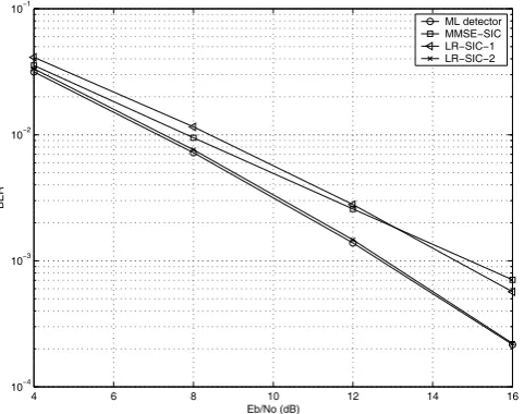
Fig. 1. BER versus SNR performance over a frequency-flat channel using Nt= 2, Nr = 2, QPSK. The channel was assumed to be perfectly known

at the receiver.

10 12 14 16 18 20 22

10Ŧ4 10Ŧ3

10Ŧ2 10Ŧ1

Eb/No (dB)

BER

ML detector MMSEŦSIC LRŦSICŦ1 LRŦSICŦ2

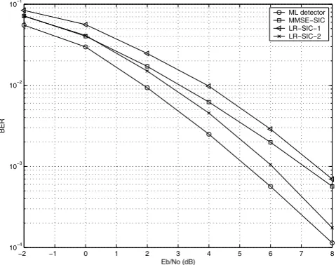
Fig. 2. BER versus SNR performance over a frequency-flat channel using Nt= 2, Nr= 2, 16-QAM. The channel was assumed to be perfectly known

at the receiver.

IV. SIMULATIONRESULTS

We have performed computer simulations to evaluate the per-formance of the LR-aided SIC detection algorithm advocated. We have assumed that all elements of the channel matrix H are independent and identically distributed (i.i.d.) zero-mean complex Gaussian random variables having a variance of 1/2 per dimension, which are known at the receiver. The LLL algorithm was used for lattice-reduction and it was applied to the extended channel matrix

[ ˜HT_σ

vIN/σx˜]T, rather than H˜T, for the sake of improving the performance [6]. Here, σx˜ denotes the standard deviation of the elements ofx˜ andIN represents the(N×N) identity matrix. Let Eb/N0 be the ratio of the average transmit power per information bit to the spectral density of the noise.

Figs. 1-4 characterize the achievable bit error rate (BER) perfor-mance of various detectors. The LR-SIC-1 scheme represents the LR-aided MMSE-SIC detector using no updating of the mean and covariance. More explicitly, at each detection stage, the LR-SIC-1 scheme uses the specific sub-matrices of the initial m and R

matrices corresponding to the symbols to be detected at a later SIC detection stage as the mean and covariance without considering the effect of the already detected symbols on them. By contrast, the LR-SIC-2 arrangement represents the LR-aided MMSE-SIC detector using the explicit updating operation derived in Section III under the assumption that the effective symbols are biased and correlated Gaussian random variables. Furthermore, the MMSE-SIC scheme denotes the MMSE version of the SIC detector of [3]. Finally, the ML detector finds the specific MIMO symbol vector having the minimum Euclidean distance from the received signal.

More specifically, Fig. 1 illustrates the four detector’s BERs for

Nt = 2, Nr = 2 and QPSK signaling for transmission over a frequency-flat channel. Observe in Fig. 1 that the performance of LR-aided detector can be significantly improved by updating both the bias and correlation of s according to (19) and (20). Hence, it becomes capable of approaching performance of the ML detector in conjunction withNt= 2,Nr= 2and QPSK signaling. As argued in Section III, for a low number of transmit antennas the Gaussian model of the effective symbols is somewhat inaccurate. Nonetheless, Fig. 1 demonstrates that we still attain an approximately 2 dB performance improvement even forNt= 2for the LR-SIC-2 scheme.

To probe a little further, Fig. 2 shows the attainable BER perfor-mance forNt= 2, Nr= 2and 16-QAM signaling. The LR-SIC-2 detector now exhibits a 0.9 dB Eb/N0 gain compared to the LR-SIC-1 scheme at BER=10−3, but now it performs 0.7 dB worse than the ML scheme.

In Fig. 3 and Fig. 4, the performance of the Nt= 4andNr= 4 scheme is shown for updating of QPSK and 16-AM constellations, respectively. It is observed that the explicit updating of the bias and covariance ofsat each detection stage provides a 1-1.5 dB gain for the LR-aided SIC detector usingNt= 4andNr= 4antennas. For Nt= 4, the Gaussian model of the effective symbols may be more accurate than the case ofNt= 2in Fig. 1 and Fig. 2. However, as the number of transmit antennas increases, the SIC detector performs worse with respect to the ML detector. This can be seen by comparing the results of MMSE-SIC in Fig. 1 and Fig. 3. This effect also occurs in the LR-SIC, and hence the SNR disadvantages of LR-SIC-2 in Fig. 3 and Fig. 4 are higher than those in Fig. 1 and Fig. 2 despite the more accurate model of the effective symbol.

V. CONCLUSIONS

In this paper, the optimal lattice-reduction aided SIC detection algorithm designed for MIMO systems has been derived. Explicitly updating the bias and covariance of the effective symbols at each SIC detection stage, where the effective symbols were generated by lattice reduction, we arrive at the optimal MMSE-SIC detector weight. At each detection stage, we update the means and covariances of (19) and (20) using the knowledge of the detected effective symbolss of (23) under the assumption that the effective symbols are jointly Gaussian distributed. We have also shown that the SIC algorithm advocated may be equivalently expressed with the aid of the extended channel matrix and received signal vector of (25) and (26), respectively. The simulation results demonstrated that the explicit updating of the mean and variance of the effective symbols after each detection stage attains an attractive performance improvement in the context of LR-aided detection, which results in a near-ML detection performance.

REFERENCES

[2] L. Hanzo, M. M¨unster, B. J. Choi, and T. Keller,OFDM and MC-CDMA for Broadband Multi-user Communications, WLANs and Broadcasting. IEEE Press - John Wiley & Sons Ltd., 2003.

[3] P. W. Wolniansky, G. J. Foschini, G. D. Golden, and R. A. Valenzuela, “V-BLAST: An architecture for realizing very high data rates over the rich-scattering wireless channel,” inProc. IEEE ISSSE-98, Pisa, Italy, Sept. 1998, pp. 295–300.

[4] X. Li, H. C. Huang, A. Lozano, and G. J. Foschini, “Reduced-complexity detection algorithms for systems using multi-element arrays,” inProc. IEEE Global Telecommun. Conf., San Francisco, CA, Nov. 2000, pp. 1072–1076.

[5] C. Windpassinger and R. F. H. Fischer, “Low-complexity near-maximum-likelihood detection and precoding for MIMO systems using lattice reduction,” inProc. IEEE Information Theory Workshop (ITW), Paris, France, March 2000, pp. 345-348.

[6] D. W¨ubben, R. B¨ohnke, V. K¨uhn, and K. D. Kammeyer, “Near-maximum-likelihood detection of MIMO systems using MMSE-based lattice-reduction,” inProc. IEEE International Conference on Communi-cations, Paris, France, June 2004, pp. 798–802.

[7] I. Berenguer, J. Adeane, I. J. Wassell, and X. Wang “Lattice-reduction-aided receivers for MIMO-OFDM in spatial multiplexing systems,” in Proc. IEEE International Symposium on Personal, Indoor and Mobile Radio Communications, Barcelona, Spain, Sept. 2004, pp. 1517-1521. [8] A. K. Lenstra, H. W. Lenstra, Jr., and L. Lov´asz, “Factoring polynomials

with rational coefficients,” Mathematische Annalen, vol. 261, pp. 515– 534, 1982.

[9] L. Afflerbach and H. Grothe, “Calculation of Minkowski-reduced lattice bases,” Computing, vol. 35, pp. 269–276, 1985.

[10] M. Seysen, “Simultaneous reduction of a lattice basis and its reciprocal basis,” Combinatorica, vol. 13, pp. 363–376, 1993.

[11] J. L. Melsa, D. L. Cohn, Decision and Estimation Theory. New York: McGraw-Hill, 1978.

[12] G.H. Golub and C.F. Van Loan, Matrix Computations, Johns Hopkins University Press, Baltimore, 1996.

[13] F. L. Lewis, Optimal Estimation with an Introduction to Stochastic Control Theory, John Wiley and Sons, New York, 1986.

[14] R. B¨ohnke, D. W¨ubben, V. K¨uhn, and K. D. Kammeyer, “Reduced complexity MMSE detection for BLAST architectures,” inProc. IEEE Global Telecommun. Conf., San Francisco, CA, Dec. 2003, pp. 2258– 2262.

APPENDIXI

Equation (22) can be rewritten as

dn=

ˆ

(GT

n,ndGn,nd+σ2vR−n1)−1 ·GT

n,nd(˜yn−Gn,ndmn) +mn

˜

1 (27)

=h(GT

n,ndGn,nd+σ2vR−n1)−1(GTn,ndy˜n+σv2R−n1mn)

i

1. (28)

Substituting (19) into (28), we arrive at

dn=

ˆ

(GT

n,ndGn,nd+σ2vR−n1)−1

˘

GT n,nd˜yn −σv2Πn,21(ˆsn,d−mn,d) +σ2vR−n1mn,nd

¯˜

1, (29) which can be rewritten as

dn=

ˆ

(GT

n,ndGn,nd+σ2vR−n1)−1

˘_GT

n,nd(˜yn−Gn,ndmn,nd) −σv2Πn,21(ˆsn,d−mn,d)

¯

+m_n,nd˜

1. (30) UsingΠn,21=CTn,ndCn,d, we obtain

GT

n,nd( ˜yn−Gn,ndmn,nd)−σ2vΠn,21(ˆsn,d−mn,d) =

[GT

n,nd σvCTn,nd]

»

˜

yn−Gn,ndmn,nd −σvCn,d(ˆsn,d−mn,d)

–

. (31)

Furthermore, we have

GT

n,ndGn,nd+σ2vRn−1= [GTn,nd σvCTn,nd]

»

G_n,nd σvCn,nd

–

.

(32)

Upon substituting (31) and (32) into (30), we obtain (24).

Ŧ2 Ŧ1 0 1 2 3 4 5 6 7 8

10Ŧ4 10Ŧ3 10Ŧ2 10Ŧ1

Eb/No (dB)

BER

ML detector MMSEŦSIC LRŦSICŦ1 LRŦSICŦ2

Fig. 3. BER versus SNR performance over a frequency-flat channel using Nt= 4, Nr= 4, QPSK. The channel was assumed to be perfectly known

at the receiver.

3 4 5 6 7 8 9 10 11 12 13

10Ŧ5 10Ŧ4 10Ŧ3 10Ŧ2 10Ŧ1

Eb/No (dB)

BER

ML detector MMSEŦSIC LRŦSICŦ1 LRŦSICŦ2

Fig. 4. BER versus SNR performance over a frequency-flat channel using Nt= 4, Nr= 4, 16-QAM. The channel was assumed to be perfectly known