JENNIFER HACKETT and GRAHAM HUTTON,
University of Nottingham, UKParametricity, in both operational and denotational forms, has long been a useful tool for reasoning about program correctness. However, there is as yet no comparable technique for reasoning about program improve-ment, that is, when one program uses fewer resources than another. Existing theories of parametricity cannot be used to address this problem as they are agnostic with regard to resource usage. This article addresses this problem by presenting a new operational theory of parametricity that is sensitive to time costs, which can be used to reason about time improvement properties. We demonstrate the applicability of our theory by showing how it can be used to prove that a number of well-known program fusion techniques are time improvements, including fixed point fusion, map fusion and short cut fusion.
CCS Concepts: •Software and its engineering→Functional languages;Polymorphism; •Theory of computation→Operational semantics;
ACM Reference Format:
Jennifer Hackett and Graham Hutton. 2018. Parametric Polymorphism and Operational Improvement. N/A, ICFP ( July 2018), 24 pages. https://doi.org/10.1145/nnnnnnn.nnnnnnn
1 INTRODUCTION
Parametric polymorphism is everywhere. In typed functional languages, many if not most of the
built-in and user-defined functions are parametric. Because of this ubiquity, we must carefully study
the properties of parametric functions. Chief among these properties is theabstraction theorem [Reynolds 1983], which shows that any well-typed term must satisfy a property that can be derived
uniformly from its type. By instantiating this theorem for specific types, we obtain the so-called
“free theorems” of Wadler [1989], properties held by any term of a given type.
The abstraction theorem was first presented by Reynolds [1983], who proved it using the notion
ofrelationalparametricity. In relational parametricity, one starts with a denotational semantics based on sets (or more generally, some form of domain) and builds on top of it another denotational
semantics based on relations between those sets. It can then be shown that interpreting any term
in related contexts must produce related results. Deriving the free theorem is then a matter of
calculating the relational interpretation of the type in question.
The original denotational presentation of the abstraction theorem is promising, as it suggests
that similar theorems will exist for any System F-like language. However, it is often not obvious
what a parametric model of such a language should be. For this reason, it is helpful to investigate
moreoperationalnotions of parametricity such as the version developed by Pitts [2000], where the relations we work with are between terms rather than between the interpretations of terms. The
result is an abstraction theorem that respects observational equivalence, provided the relations
involved satisfy the intuitive property of⊤⊤-closure.
Authors’ address: Jennifer Hackett; Graham Hutton, School of Computer Science, University of Nottingham, Jubilee Campus,
Wollaton Road, Nottingham, NG8 1BB, UK, {jennifer.hackett, graham.hutton}@nottingham.ac.uk.
Permission to make digital or hard copies of all or part of this work for personal or classroom use is granted without fee
provided that copies are not made or distributed for profit or commercial advantage and that copies bear this notice and
the full citation on the first page. Copyrights for components of this work owned by others than ACM must be honored.
Abstracting with credit is permitted. To copy otherwise, or republish, to post on servers or to redistribute to lists, requires
prior specific permission and /or a fee. Request permissions from [email protected].
© 2018 Association for Computing Machinery.
XXXX-XXXX/2018/7-ART $15.00
Parametricity can be used to give correctness proofs of a number of useful program optimisations,
most notably short cut fusion [Gill et al. 1993]. However, correctness is only one side of optimisations:
we must also consider whether transformationsimproveperformance. In order to carry correctness results into this setting we need aresource-awaretheory of parametricity, to provide us with free theorems that include information about efficiency properties.
In this article we develop a new operational theory of parametricity that can be used to reason
abouttime improvement, i.e. when one term can be replaced by another without increasing time cost. Our theory is built on a standard lazy abstract machine [Sestoft 1997], making it applicable to
call-by-need languages such as Haskell. Specifically, we make the following contributions:
• We show how Pitts’ notion of⊤⊤-closure can be adapted to produce a resource-aware notion
that we call machine-closure. The key idea is that whereas ⊤⊤-closed relations respect
observational equivalence, machine-closed relations respecttime improvement.
• We use the notion of machine-closure to prove an abstraction theorem for call-by-need programs that use recursion in a restricted manner, namely when the right-hand side of the
recursive binding is invalueform. The resulting theorem can be used to reason about time improvement properties in call-by-need languages such as Haskell.
• We demonstrate the application of our abstraction theorem by justifying a number of
fusion-based optimisations as time improvements, including short cut fusion. We focus on fusion as
most parametricity-based optimisations are instances of fusion.
This work has similar aims to that of Seidel and Voigtländer [2011], who investigate
efficiency-based free theorems in a call-by-value language, but differs in setting and approach. Firstly, we
consider call-by-need rather than call-by-value. Secondly, their work is based on a denotational
semantics instrumented with costs and it is not clear how this can be applied in a call-by-need
setting, so instead we use an operational semantics with an explicit stack and heap. Finally, our work
builds on the call-by-need improvement theory of Moran and Sands [1999a], using an improvement
relation to abstract away from explicit costs where possible.
This paper is part of a wider project to make questions of call-by-need efficiency more tractable
[Hutton and Hackett 2016]. By developing new techniques for questions of improvement that are
compatible with the existing techniques used to prove correctness, we seek to bring the two issues
of correctness and improvement closer together, reducing the work that must be done to formally
justify a particular program transformation. In this case, a technique based on parametricity for
reasoning about improvement makes it easier to reason about the efficiency aspects of program
transformations that rely on parametricity for their correctness properties.
2 BACKGROUND
We begin in this section with some background on the two key technical elements that underpin
our work, namely parametric polymorphism and operational improvement.
2.1 Parametric Polymorphism
The viewpoint of parametric polymorphism is that a polymorphic function must do thesamething at every type. This contrasts with ad-hoc polymorphism [Strachey 2000], where it is only required
that a function dosomethingat every type. The result is that parametrically polymorphic functions are forced to respect the abstractions of the calling code, being prevented from inspecting the
structure of the type at which they are called. This property was first observed by Reynolds [1983],
who proved theabstraction theoremfor the polymorphicλ-calculus.
Reynolds’ abstraction theorem works by first defining a set-theoretic denotational semantics,
this a semantics oflogical relations. These relations are built by defining relation-lifted definitions of the type constructors of the language. For example, two terms at a function type are related if
they take related arguments to related results:
(f,g) ∈R→S ⇔ ∀(x,y) ∈R. (f x,g y) ∈S
Once we have this relational interpretation of types, it can be shown by a straightforward induction
on the structure of type derivations that interpreting any term in related environments will give
related results. This model can be extended with extra constructs such as general recursion and
sequencing, which translate to adding restrictions on the relations [Johann and Voigtländer 2004].
However, this method is limited to languages with a natural denotational semantics, and so cannot
be applied when the only natural semantics is operational.
Pitts [2000] addressed this issue by presenting anoperationaltreatment of parametricity for a language called PolyPCF, a version of Plotkin’s PCF [Plotkin 1977] extended with list types and
polymorphism. The same technique of building relations from the structure of types is used, but
these relations are between terms rather than elements of a denotational semantics. It is therefore
necessary to require that the relations respect equivalence in the operational semantics.
To ensure that relations respect equivalence, Pitts introduced two notions for PolyPCF language.
Firstly, there is the⊤relation that holds between stacks (which function as term contexts) and
terms whenever the stack applied to the term will produce the empty listNil. Secondly, there is the
⊤⊤-closure operator for term relations, so called because it involves using the⊤relation twice:
once to go from a relation on terms to one on stacks, and once to go back again. As a consequence
of the definition, all⊤⊤-closed relations respect equivalence.
We can summarise the notion of⊤⊤-closure as follows. Given a relationR:τ1↔τ2between
typesτ1andτ2, its⊤⊤-closureR
⊤⊤
is a relation of the same type. A pair(M1,M2)is inR⊤⊤if: for all stacksS1,S2,
if for all(N1,N2) ∈R,S1⊤N1⇔S2⊤N2
thenS1⊤M1⇔S2⊤M2
Pitts shows that⊤⊤-closed relations are closed under the relational versions of function space
formation, type abstraction and list type formation, thus demonstrating that they are a suitable
notion of relation on terms. It can then be shown that any closed term is related to itself, and that
open terms are related to themselves provided that the relational interpretations of the free type
variables are all⊤⊤-closed. Applying this theorem is then a matter of instantiating with particular
relations, provided these relations can be shown to be⊤⊤-closed.
2.2 Operational Improvement
In order to reason about the operational efficiency of programs, we need some model of the cost of
terms. For call-by-value this is straightforward: in most cases it is enough simply to count the steps
taken to evaluate the term to normal form; functions are slightly more complicated as we have
both the cost to evaluate the function itself and the cost to compute its result, where the latter may
depend on the argument to the function [Shultis 1985]. The result is a semantics of call-by-value λ-terms that can be used to reason about time costs.
The situation for call-by-need is more complicated, however. In this case, a subterm is only
evaluated when it isforced, i.e. when its value is required, so the cost to evaluate a term to normal form is a poor measure of efficiency. For example, the terms[⊥]and[0]are both in normal form,
evaluating subterms as well, but this method will identify the termsletx=Min(x,x)and(M,M) even though one shares work in a way the other does not.
The solution of Moran and Sands [1999a] is to quantify over evaluation contexts. That is to say,
a termMisimproved byanother termN, writtenM ▷
∼N, if for all contextsC, the termC[M]takes at least as many steps to evaluate asC[N]. By taking into account all possible uses of the initial terms, we automatically take into account cost savings introduced by sharing as well as the cost of
computing subterms. Furthermore, this notion of efficiency is compositional by definition, making
it amenable to techniques of inequational reasoning.
Moran and Sands’ improvement theory has been used to justify general-purpose program
improvements, such as the worker/wrapper transformation [Hackett and Hutton 2014]. This takes
advantage of the parallels between the rules of call-by-need improvement and those of program
equivalence, which makes it possible to adapt proofs of correctness into proofs of improvement. Subsequent work took this idea of having compatible equivalence and improvement proofs and
placed it in a generalised setting ofpreorder-enriched categories[Hackett and Hutton 2015]. Improvement theory and related techniques have seen something of a resurgence in recent years.
Breitner [2015] uses an operational approach to proving the safety of the call arity transformation
based on counting the number of allocations made. Sergey et al. [2017] use a step-counting approach
to show that floatingletbindings into a lambda is an improvement provided the lambda expression
is used only once. Schmidt-Schauß and Sabel [2015] use an operational semantics based on term
rewriting rules to show that a number of local optimisations are improvements, including common
subexpression elimination. Finally, Simões et al. [2012] define a cost model for Launchbury’s natural
semantics [Launchbury 1993], and use it to prove soundness of a cost analysis.
3 FROM EQUIVALENCE TO IMPROVEMENT
In this section, we show how to build a theory of parametricity that can be used to reason about
program improvements. Essentially we want to do for improvement what Pitts did for equivalence.
Unfortunately, Pitts’ notion of⊤⊤-closure is too strong for our purposes: because⊤⊤-closed
relations must respect program equivalence, they cannot be used to distinguish between
obser-vationally equivalent programs with different costs. In a sense, Pitts’ notion of observation is too
narrow for our purposes. What we need is a notion of closure that forces relations to respect only
cost-equivalence, i.e. when two programs are interchangeable in terms of time costs.
3.1 Call-By-Need PolyPCF
We consider a simple language, a polymorphically-typedλ-calculus with recursive bindings. The
type and term grammars are defined as follows:
α ∈TVar
x,y,xs∈Var A,B∈Type::=α
| A→B | List A | ∀α.A
M,N ∈Term::= x | λx.M | M x | Λα.M | M A
| let{ ®x =M®}inN | Nil
| x::xs
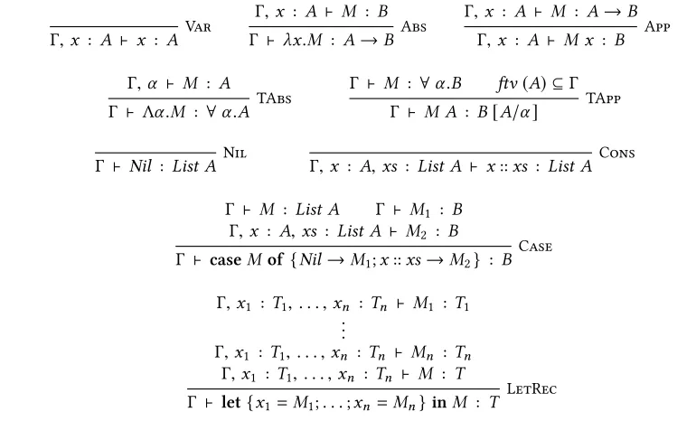
The typing rules for the language are given in Figure 1, and comprise one rule for each language
construct. Note that the typing contextΓcontains both free type variables and type assignments for free term variables. We apply a standard well-formedness constraint toΓ.
Our chosen language is similar to the PolyPCF language studied by Pitts, but with two key
differences. Firstly, we have added recursive let-bindings to the language and remove the fixed
point combinatorfix. We do this because let-binding-based presentations of recursion are better at capturing sharing. Secondly, we only allow functions and constructors to be applied to variables.
This latter distinction is useful because it means that all sharing is explicitly introduced in
let-bindings, making it easier to reason about call-by-need evaluation; a similar restriction applied to
earlier versions of the internal language used in the Glasgow Haskell Compiler, GHC Core.
The operational semantics for this language is a small-step semantics based on Sestoft’s Mark 1
abstract machine [Sestoft 1997], extended to handle type abstraction and application. A machine
state is given by a triple⟨H,M,S⟩consisting of a heapHthat binds term variables to terms, the current term to be evaluatedM, and a stackSconsisting of tokens that describe the context in which the result of evaluatingMis to be used. There are four kinds of stack tokens: variable updates #xthat signal when a variable is to be updated with the result of the computation; applicationsx that signify when the result should be given a variable as an argument; type applications[A]that signify when the result should be given atypeargument; and finally, alternativesaltsthat signify that the result should be pattern-matched and branched on.
A term is considered evaluated when it is invalue form, that is, when it is the empty list, a cons cell or either kind of abstraction. Note that this is quite a restrictive form for lists, as cons cells
only contain variables rather than terms; this reflects the fact that a fully-evaluated list will exist
almost entirely on the heap. By convention, we denote value terms with letters such asV andW.
The complete set of transition rules for the semantics are given in Figure 2. We assume that all
bound variables are unique in the statement of these rules, which can be achieved byα-renaming
to a fresh variable whenever an abstraction is opened.
Now we can define our notions of improvement and cost-equivalence. If for all heaps and stacks
⟨H,S⟩we have that if⟨H,M,S⟩terminates after makingnLookup steps then⟨H,N,S⟩terminates afternor fewer Lookup steps, we sayMisimprovedbyN, writtenM▷
∼N. IfMandNboth improve each other we say that they arecost-equivalent, writtenM◁▷
∼ N. Note that improvements capture the notion ofnever-worse, and do not guarantee that the resulting term is in practicebetter.
We only count Lookups as these are an appropriate measure of the total cost of evaluating
a term. In particular, the total number of steps is bounded by a linear function of the number
of Lookups [Moran and Sands 1999a]. Of course, it may be the case that an improvement that
holds when counting Lookups fails when taking some other operational aspects into account.
However, restricting the scope of the costs makes the theory more tractable. This is standard in
improvement theory – no abstract model will perfectly match reality, and given that memory access
often dominates, counting memory accesses is a reasonable approach.
3.2 Machine-Closure for Relations
Now that we have our language, we must develop a notion of relations between terms of that
language. These relations will be between terms of particular types in the language; ifRrelates terms of typeAto terms of typeB, we say thatRhas the typeA↔B. However, not all relations will have the desired properties of respecting costs. We must therefore have some notion ofpermissible relations that are all guaranteed to have this property.
As noted above, we cannot use Pitts’ notion of⊤⊤-closure as it identifies all equivalent terms
regardless of cost. However, we can modify⊤⊤-closure to produce another notion of closure that
Γ,x : A ⊢ x : A Var
Γ,x : A ⊢ M : B
Γ ⊢ λx.M : A→B Abs
Γ,x : A ⊢ M : A→B
Γ,x : A ⊢ M x : B App
Γ,α ⊢ M : A
Γ ⊢ Λα.M : ∀α.A TAbs
Γ ⊢ M : ∀α.B ftv(A) ⊆Γ
Γ ⊢ M A : B[A/α]
TApp
Γ ⊢ Nil : List A Nil
Γ,x : A,xs : List A ⊢ x::xs : List A Cons
Γ ⊢ M : List A Γ ⊢ M1 : B
Γ,x : A,xs : List A ⊢ M2 : B
Γ ⊢ caseMof {Nil→M1;x::xs→M2} : B Case
Γ,x1 :T1, . . . ,xn :Tn ⊢ M1 :T1 ..
.
Γ,x1 :T1, . . . ,xn :Tn ⊢ Mn :Tn
Γ,x1 :T1, . . . ,xn :Tn ⊢ M : T
[image:6.486.53.438.89.322.2]Γ ⊢ let{x1=M1;. . .;xn =Mn}inM : T LetRec
Fig. 1. The typing rules for our language
⟨H {x=M},x,S⟩ → ⟨H,M,#x : S⟩ { Lookup }
⟨H,V,#x : S⟩ → ⟨H {x=V},V,S⟩ { Update }
⟨H,M x,S⟩ → ⟨H,M,x : S⟩ { Unwind }
⟨H,λx.M,y : S⟩ → ⟨H,M[y/x],S⟩ { Subst }
⟨H,M A,S⟩ → ⟨H,M,[A] : S⟩ { TypeUnwind }
⟨H,Λα.M,[A] : S⟩ → ⟨H,M[A/α],S⟩ { TypeSubst }
⟨H,caseMof alts,S⟩ → ⟨H,M,alts : S⟩ { Case }
⟨H,Nil,{Nil→N1;x::xs→N2} : S⟩ → ⟨H,N1,S⟩ { BranchNil } ⟨H,y::ys,{Nil→N1;x::xs→N2} : S⟩ → ⟨H,N2[y/x,ys/xs],S⟩ { BranchCons } ⟨H,let{ ®x=M®}inN,S⟩ → ⟨H { ®x =M®},N,S⟩ { Letrec }
Fig. 2. The call-by-need abstract machine
stack pairsthat capture all of the state of the abstract machine besides the term itself, and adapting the⊤relation to take costs into account. We also follow Voigtländer and Johann [2007] and use
one-directional implication in our definition, as this is more useful for reasoning about program
orderings. We call the resulting notion of closuremachine-closure. Given a relationR : A↔B, two termsM1 : AandM2 : Bare related by the machine-closure ofR, writtenR
M, if:
for all heap and stack pairs⟨H1,S1⟩and⟨H2,S2⟩,
[image:6.486.54.443.371.503.2]By⟨H,N,S⟩ ↓n, we mean that if we start the abstract machine in state⟨H,N,S⟩, then it will take at mostnLookup steps to finish evaluating. The key idea is that machine-closed relations should only be able to capture properties that can be observed by running terms in specific machine contexts
and comparing the costs. In other words, they must beobservational improvementproperties. We can prove a number of useful theorems about closure. Firstly, we note that
machine-closure is monotone, i.e. ifR⊆SthenRM ⊆SM. This follows from the fact thatRappears twice under the left-hand side of an implication. Secondly, we show that machine-closure reallyisa notion of closure, i.e.R⊆RM=(RM)M. ThatRis smaller thanRMfollows from the definition, as when(M1,M2) ∈Rthen the criterion for membership inRMbecomes a tautology. Then, as any heap and stack pairs that identify pairs inRwill also identify pairs inRMby definition, we can conclude that any pair in(RM)Mwill also be inRM, so our closure operation is idempotent.
Finally, we show that machine-closed relations respect improvement, in the sense that whenever
(M1,M2) ∈R,M′
1∼▷M1andM2▷∼M
′
2, then(M
′
1,M
′
2) ∈R. Assuming this precondition, and assuming Ris machine closed, we can then conclude that for any heap and stack pairs⟨H1,S1⟩and⟨H2,S2⟩ such that for any(N1,N2) ∈R, we have⟨H1,N1,S1⟩ ↓n⇒ ⟨H2,N2,S2⟩ ↓n:
⟨H1,M′
1,S1⟩ ↓n ⇒ { improvement }
⟨H1,M1,S1⟩ ↓n ⇒ { assumption }
⟨H2,M2,S2⟩ ↓n ⇒ { improvement }
⟨H2,M2′,S2⟩ ↓n
Therefore, we can conclude that(M′
1,M
′
2)is also inR
M.
3.3 Actions on Relations
Now that we have defined an appropriate notion of relation on terms, we must in turn define how
the type constructors of our language act on those relations. In particular, we need these actions
to preserve the machine-closure property, in order that any relation built out of machine-closed
relations using these constructors will also be machine-closed. We can define relational actions for
the three type constructors of our language as follows:
• Function spaces.Given relations,R : T1↔T
′
1andS :T2↔T
′
2, we can define the relation R→S : (T1→T2) ↔ (T
′
1 →T
′
2). Two termsM :T1→T2andM
′ :T′
1 →T
′
2are related by R→Siff for all collections of bindingsB,B′, we have the following implication:
(letBiny,letB′iny) ∈R
⇒ (letBinM y,letB′inM′y) ∈S
In other words, they must take related arguments to related results.
• List types.GivenR : T ↔T′, we can define the relationList R : List T ↔List T′as the least fixed point of the following equation, for all collections of bindingsB,B′:
List R=({ (Nil,Nil) } ∪
{ (letBiny::ys,letB′iny::ys) | (letBiny,letB′iny) ∈R,
In other words,Nilis related to itself, and non-empty lists are related if their heads and tails are related. The fixed point is guaranteed to exist because all operations in the definition are
monotone and relationsList A↔List A′form a lattice.
• Type abstraction.Given a family of functionsRindexed over typesT1,T′
1that map relations
of typeT1↔T
′
1to relations of typeT2[T1] ↔T
′
2 [T
′
1], we can define the relation∀r. R(r).
Two termsM : ∀α.T2[α]andM
′ :
∀α.T2′[α]are related by∀r. R(r)if and only if: ∀T1,T1′∈Type,S :T1↔T
′
1 . (MT1,M′T′
1) ∈R(S)
In other words, two polymorphic terms are related if a relation between two types can be
lifted to a relation that relates the terms’ instantiations at those types.
These three definitions are based on the relational actions from Pitts [2000], adapted to our setting.
We use the technique of adding bindings to get around the limitation of applying terms and
constructors only to variables, and to take account of sharing. There is an implicit requirement in
the above definitions that all the bindings are type-correct. Note that our approach for lists differs
from that of Pitts, who uses agreatestfixed point to make the use of coinduction easier. In contrast, we use a least fixed point to make the use of induction easier. In Pitts’ setting, both definitions
result in the same logical relation, and we conjecture the same is true in our setting. However, our
theory does not depend on this being the case, and all of our results hold regardless.
The next step is to prove that all three of these constructions preserve the notion of
machine-closure. That this is the case for theListconstruction is immediate, as any fixed-point of the defining equation is by definition machine-closed. For the other two, the proof is a little more involved:
Lemma 3.1 (Function Space Preserves Machine-Closure).
(i) Given bindings B, B′and heap and stack pairs⟨H,S⟩,⟨H′,S′⟩, if we have (a) (letBiny,letB′iny) ∈R
(b) ∀(N,N′) ∈R′.⟨H,N,S⟩ ↓n⇒ ⟨H′,N′,S′⟩ ↓n then we also have
∀(M,M′) ∈R→R′ .
⟨H+B,M,y : S⟩ ↓n⇒ ⟨H′+B′,M′,y : S′⟩ ↓n
(By H +B, we mean the heap gained by adding the bindings B to the heap H .) (ii) Given machine-closed relations R and R′, then R→R′is also machine-closed.
Proof. For part (i), take arbitrary(M,M′) ∈R→R′. We note that(letBinM y,letB′inM′y) ∈ R′by assumption (a) and the definition ofR→R′, and reason as follows:
⟨H+B,M,y : S⟩ ↓n
⇔ { Unwind and Letrec steps are free }
⟨H,letBinM y,S⟩ ↓n ⇒ { assumption (b) }
⟨H′,letB′inM′y,S′⟩ ↓n
⇔ { Unwind and Letrec steps are free }
⟨H′+B′,M′,y : S′⟩ ↓n
For part (ii), we assume(M,M′) ∈ (R→R′)Mfor machine-closedRandR′, and aim to prove
we must show that(let B in M y,let B′ in M′ y) ∈ R′. Letting⟨H,S⟩, ⟨H′,S′⟩ be arbitrary heap-stack pairs such that∀(N,N′) ∈R′.⟨H,N,S⟩ ↓n⇒ ⟨H′,N′,S′⟩ ↓n, we have:
⟨H,letBinM y,S⟩ ↓n
⇔ { Unwind and Letrec steps are free }
⟨H+B,M,y : S⟩ ↓n
⇒ { part (i), definition of machine-closure }
⟨H′+B′,M′,y : S⟩ ↓n
⇔ { Unwind and Letrec steps are free }
⟨H′,letB′inM′y,S⟩ ↓n
Because these heap-stack pairs were arbitrary, we can conclude(letBinM y,letB′inM′y) ∈
R′M, which implies the desired result by the assumption thatR′is machine-closed. □
Lemma 3.2 (Type Abstraction Preserves Machine-Closure).
(i) Given heap and stack pairs⟨H,S⟩,⟨H′,S′⟩, if we have ∀r : T ↔T′,(N,N′) ∈R(r) .
⟨H,N,S⟩ ↓n ⇒ ⟨H′,N′,S′⟩ ↓n
then we also have
∀(M,M′) ∈∀r. R(r) .
⟨H,M,[T] : S⟩ ↓n⇒ ⟨H,M′,[T′] : S′⟩ ↓n
(ii) For any typesT2,T
′
2, given a family of functions R indexed over typesT1,T
′
1that map relations of typeT1↔T
′
1to relations of typeT2[T1] ↔T
′
2 [T
′
1], if all the relations R(r)are machine-closed then the relation∀r.R(r)will also be machine-closed.
Proof. Similarly to Lemma 3.1, but with TypeUnwind steps rather than Unwind/Letrec. □
3.4 The Logical Relation
Given the above relational actions, it is possible to define a family of relations indexed over types,
abstracted over the interpretations of type variables. By convention this family is called thelogical relation, denoted∆. The idea is that this family of relations will relate every term to itself, and so by calculating the relation for a particular type we will get a property of terms of that type. This
property is called theabstraction theorem. Using the constructions from the previous section, we can define our logical relation recursively on the structure of types:
∆( ®R/ ®α) (αi) = Ri
∆( ®R/ ®α) (T1→T2) = ∆( ®R/ ®α) (T1) →∆( ®R/ ®α) (T2)
∆( ®R/ ®α) (∀α.T) = ∀r. ∆(rM/α,R®/ ®α) (T)
∆( ®R/ ®α) (List T) = List(∆( ®R/ ®α) (T))
A simple proof by induction shows that∆( ®R/ ®α) (T)is machine-closed whenever all theR®are. Furthermore, another proof by induction shows that if all ofR®are subsets of▷
∼then∆( ®R/ ®α) (T)is also a subset of▷
3.5 The Abstraction Theorem (for Non-Recursive Programs)
Now we can prove a version of the abstraction theorem. In this section we will prove the theorem
for a non-recursive version of our language, but in the next section we will show how to extend
the theorem to deal with recursive programs. We proceed in this manner because dealing with
recursion requires applying some limitations to our language that we do not wish to apply to
non-recursive programs. For the purposes of this section, we use the following weaker version of
the Let rule that disallows the use of recursion:
Γ ⊢ M1 :T1 . . . Γ ⊢ Mn :Tn
Γ,x1 :T1, . . . ,xn :Tn ⊢ M : T
Γ ⊢ let{x1=M1;. . .;xn =Mn}inM : T Let’
Now we state the abstraction theorem:
Theorem 3.3 (Abstraction for Non-Recursive Programs). Given a closed term M and closed type A such that ⊢ M : A (using the weaker Let’ rule rather than Let), we have(M,M) ∈∆() (A).
To prove this theorem we must actually prove a stronger theorem, extending the logical relation
∆to terms with free variables. AssumingΓ=α®,x1 :T1, . . . ,xn :Tn, we defineΓ ⊢ M ∆ M
′ : T to mean that for all bindingsB,B′that close the termsM,M′respectively, and machine-closed relationsR® :Ti ↔T′
i (wherelengthR®=lengthα®), we have: (∀i∈ [1. .n] .
(letBinxi,
letB′inxi) ∈∆( ®R/ ®α) (Ti)) ⇒
(letBinM[ ®T/ ®α],
letB′inM′[ ®T′/ ®α]) ∈∆( ®R/ ®α) (T)
Theorem 3.3 then follows immediately from the following lemma:
Lemma 3.4. Given a contextΓ, term M and type A such thatΓ ⊢ M : T (using the weaker Let’ rule instead of Let), we have thatΓ ⊢ M ∆ M : T . (The proof is given in the Appendix.)
4 DEALING WITH RECURSIVE BINDINGS
In order to extend our treatment to deal with the full Let rule, we must have some way to reason
about the behaviour of recursive bindings. The usual technique, as used by Pitts [2000] and Moran
and Sands [1999a], is to define some notion of unwinding and to consider a fixed point as a limit to
the sequence of increasingly deep unwindings. This notion of limit is made precise by anunwinding lemmathat relates the behaviour of recursive terms to that of their finite non-recursive unwindings. For example, the meaning ofletx=MinNis generally taken to be the limit of the sequence:
letx0=⊥inN [x0/x]
letx1=M[x0/x];x0=⊥inN [x1/x]
letx2=M[x1/x];x1=M[x0/x];x0=⊥inN[x2/x] ..
We denote thenth element of this sequence asletx=n MinN
This technique cannot be applied as-is in a call-by-need setting, as there is work shared in the
recursive definition that is not shared in any of the unwindings. We follow the approach taken by
Moran and Sands [1999a] and restrict ourselves to cases where the right-hand side is a value, in
which case the problem does not arise. We return to this assumption in the concluding section.
First of all, we must state and prove our version of the unwinding lemma. In this case, we want
to know that machine-closed relations behave well with respect to limits of unwindings, which can
be regarded as a kind of continuity property of relations.
Lemma 4.1 (Unwinding).
(i) A machine state⟨H {x=V},N,S⟩terminates in k steps iff there is some non-negative integer n such that the machine state⟨H {x=n V},N,S⟩terminates in k steps.
(ii) Given a pair of closed termslet x = V in N andlet x = V′ in N′and a machine-closed relation R, the membership relation(let x =V in N,let x = V′ in N′) ∈ R holds iff the membership relation(letx=nV inN,letx=n V′inN′) ∈R holds for all non-negative n.
Proof. Part (i) follows easily from the fact that a binding can only recurse finitely many times
in a given execution. For part (ii), the⇒direction follows from (i) and the definition of
machine-closure. For the⇐direction, suppose we have heap and stack pairs⟨H1,S1⟩and⟨H2,S2⟩such that for any(P,P′) ∈ R, we have⟨H1,P,S1⟩ ↓n⇒ ⟨H2,P′,S2⟩ ↓n. We prove that⟨H1,let x = V inN,S1⟩ ↓n⇒ ⟨H2,letx=V′inN′,S2⟩ ↓nby case analysis on the termination behaviour of the left-hand side of this result, considering the two cases in turn:
• Termination. If⟨H1,letx=V inN,S1⟩terminates inksteps, then by part (i) there must be some non-negative integernsuch that⟨H1,letx=n V inN,S1⟩terminates inksteps, in which case we also have that⟨H2,letx=n V′inN′,S2⟩terminates inksteps, and then by part (i) we can conclude that⟨H2,letx =V′inN′,S2⟩terminates inksteps.
• Non-termination. If⟨H1,letx=V inN,S1⟩does not terminate,⟨H1,letx=V inN,S1⟩ ↓n
⇒ ⟨H2,letx=V′inN′,S2⟩ ↓nis vacuously true. □
Now we can extend our proof of Lemma 3.4 to deal with recursive bindings. Only the Let case
differs. For simplicity, we illustrate the case for a single recursive binding, but the result can be
generalised easily to the case of multiple recursive bindings.
Lemma 4.2 (Recursive bindings). If Γ,x :T1 ⊢ V ∆V :T1andΓ,x :T1 ⊢ N ∆N :T2both hold, thenΓ ⊢ letx=V inN ∆letx=V inN :T2will also hold.
Proof. LetB andB′ be bindings that closelet x = M in N (but don’t containx; we can ensure this with alpha-renaming) and letR® : T® ↔ ®T′ be a list of machine-closed relations with length equal to the number of free type variables inΓ. Assume that for anyy : A ∈ Γ, we have (let B in y,let B′ in y′) ∈ ∆ ( ®R/ ®α) (A). We aim to prove (let B in let x = V [ ®T/α]inN [ ®T/α],letB′in letx =V [ ®T′/α]inN [ ®T′/α]) ∈∆( ®R/ ®α) (T2).
It suffices to prove(letB;x =V [ ®T/α]inx,letB′;x =V [ ®T′/α]inx) ∈∆( ®R/ ®α) (T1), which implies our goal by the assumptionΓ,x :T1 ⊢ N ∆N :T2. First, we prove that for alln, we have (letB;x =n V [ ®T/α]inxn,letB′;x =n V [ ®T′/α]inxn) ∈∆( ®R/ ®α) (T1). We do this by induction onn. The base case is simple, as both sides diverge and all machine-closed relations relate diverging terms to each other. For the inductive case, we reason as follows. Our induction hypothesis is
that(let B;x =n V [ ®T/α] in xn,let B′;x =n V [ ®T′/α] in xn) ∈ ∆ ( ®R/ ®α) (T1), so by the assumptionΓ,x :T1 ⊢ V ∆V :T1we know that(letB;x =
V [ ®T/α] in V [xn/x]) ∈ ∆ ( ®R/ ®α) (T1). But these terms are cost-equivalent to (let B;x =n+1 V [ ®T/α]inxn,letB′;x =n+1V [ ®T′/α]inxn), so we are done.
Finally, we apply Lemma 4.1 to give(letB;x =V [ ®T/α] inx,let B′;x =V [ ®T′/α]in x) ∈
∆( ®R/ ®α) (T1), which completes the proof of this lemma. □
5 APPLICATIONS
In this section, we apply our abstraction theorem to a range of examples to derivefree theorems for improvement: theorems about the operational time efficiency of terms that rely only on their polymorphic types. As this theory is built on the same language and cost model as Moran and
Sands [1999a], all the same theorems hold, but now we have the added tool of parametricity. In
order to apply this tool, however, we need ways to construct interesting machine-closed relations.
In Moran and Sands’ theory, there is the special operator✓(which is pronounced as ‘tick’) that
adds one unit of cost. In our context, it is useful to reify this into the machine model, as this makes
reasoning easier. We therefore add a tick token✓to our stacks: it is safe to do this because our
reasoning was generic in the possible stack items. We introduce the following transition rule for✓
to the abstract machine semantics that we defined in Figure 2:
⟨H,M, ✓ : S⟩ → ⟨H,M,S⟩ { Tick }
and count these steps as well in our cost semantics, so the total cost of evaluation is now given by
the number of Lookup and Tick steps. We can then formulate the following theorem:
Theorem 5.1. Given a contextCsuch thatC[⊥]◁▷
∼ ⊥, the following relations are machine-closed:
(i) { (M,M′) |C[M]▷
∼M ′}
(ii) { (M,M′) |M ▷
∼C[M ′] }
By⊥, we mean some arbitrarily-chosen divergent term.
Proof. We take an arbitrary pair(M,M′)in the machine-closure of the relation and show it is in the original relation. For (i) we must showC[M]▷
∼M
′, which by definition is equivalent to:
∀⟨H,S⟩,⟨H,C[M],S⟩ ↓n ⇒ ⟨H,M′,S⟩ ↓n
Take an arbitrary⟨H,S⟩. Starting in the state⟨H,C [x],S⟩ wherexis fresh, the machine will either evaluate to⟨H′,x,S′⟩inksteps, or it will diverge, because otherwise it would violate the assumptionC[⊥]◁▷
∼ ⊥. If⟨H,C[x],S⟩diverges then so does⟨H,C[M],S⟩, so⟨H,C[M],S⟩ ↓n
⇒ ⟨H,M′,S⟩ ↓n is vacuously true and we are done. Otherwise, take an arbitrary(N,N′)such thatC[N]▷
∼N ′
. We know that⟨H,C[N],S⟩evaluates to⟨H′,N,S′⟩inksteps by construction, so we can conclude⟨H′,N,k✓ : S′⟩ ↓n⇒ ⟨H,C[N],S⟩ ↓n(wherek✓representskcopies of✓). From this and the assumptionC[N]▷
∼N ′
we can conclude⟨H′,N,k✓ : S′⟩ ↓n ⇒ ⟨H,N′,S⟩ ↓n. BecauseN andN′were arbitrary, by the definition of machine-closure this implies⟨H′,M,k✓ : S′⟩ ↓n⇒ ⟨H,M′,S⟩ ↓n, which by construction implies⟨H,C[M],S⟩ ↓n⇒ ⟨H,M′,S⟩ ↓n.
The second case (ii) follows the same pattern. □
5.1 Example: Fixed Point Fusion
Given a fixed point combinatorfix : ∀α. (α→α) →α, thefixed point fusionrule [Meijer et al. 1991] states that ifhis a strict function such thath·f =д·h, then we havefix f =h(fix g). We can actually prove an improving version of this rule using parametricity, solely from the type.
for any bindingsB2,B
′
2and machine-closed relationR : T ⇔T
′,
if for any bindingsB1,B
′
1we have (letB1inx,letB
′
1inx) ∈R ⇒ (letB1in(letB2inf)x,letB
′
1in(letB
′
2inf)x) ∈R
then(letB2infix T f,letB
′
2infix T
′f) ∈R
Simplifying, by lettingB2={f =M1},B
′
2={f =M2}, we obtain:
for any machine-closed relationR, if for any bindingsB1,B′
1we have (letB1inx,letB
′
1inx) ∈R ⇒ (letB1inM1x,letB
′
1inM2x) ∈R
then(letf =M1infix T f,letg=M2infix T
′g) ∈R
Now if we letR={ (N,N′) |C[N]▷
∼N ′}
, we obtain:
for any contextCsuch thatC[⊥]◁▷ ∼ ⊥, if for any bindingsB1,B
′
1we have letB1inC[x]∼▷letB
′
1inx ⇒ letB1inC[M1x]∼▷letB
′
1inM2x
thenletf =M1inC[fix T f]▷∼letg=M2infix T
′
g Finally, we observe that the preconditionletB1inC[x]▷
∼letB ′
1 inx ⇒ letB1inC[M1x]▷
∼
letB′
1inM2xis implied byletB1inC[M1x]▷∼letB1,y=C[x]inM2y, so we obtain:
for any contextCsuch thatC[⊥]◁▷ ∼ ⊥, if for any bindingsB1we have
letB1inC[M1x]▷
∼letB1,y=C[x]inM2y
thenletf =M1inC[fix T f]▷
∼letg=M2infix T
′g
Here, the role of the functionhis played by the contextC, and the requirementC[⊥]◁▷
∼ ⊥states that this context must be strict. The fixed functionsf andgcorrespond to the termsM1andM2,
and the requirement thatletB1inC[M1x]▷
∼letB1,y=C[x]inM2yis simply a spelling-out
ofh·f =д·h. Thus we see that our abstraction theorem implies an improving version of the
standard fixed point fusion rule. We can also takeR={ (N,N′) |N ▷
∼C[N
′] }to obtain a version
of this rule where the improvement goes in the other direction:
for any contextCsuch thatC[⊥]◁▷ ∼ ⊥, if for any bindingsB1we have
letB1,y=C[x]inM1y▷
∼letB1inC[M2x]
thenletf =M1infix T f ▷
∼letg=M2inC[fix T
′g]
The first rule tells us that fusion is an improvement when the fusion precondition is an improvement
in one direction. The second tells us that reverse fusion (“fission”) is an improvement when the
fusion precondition is an improvement in the other direction. Together, these imply that if the
fusion precondition is a cost equivalence, then fusion itself is a cost equivalence.
5.2 Example: Map Fusion
For our second example, consider themapfunction on lists:
map : ∀α β. (α→β) →Listα→Listβ map=Λα β.λf xs→
casexsof
Nil →Nil
A common optimisation concerning this function ismap fusion, where two successive applications ofmapare fused into one. The correctness of this transformation is a consequence of the free theorem formap, so it makes sense to ask if we can justify it as an improvement in a similar way. The abstraction theorem applied tomapgives us the following:
for any bindingsB2,B
′
2and machine-closed relationsR1 :T1↔T
′
1,R2 :T2↔T
′
2,
if for any bindingsB1,B
′
1we have (letB1inx,letB
′
1inx) ∈R1 ⇒ (letB1in(letB2inf)x,letB
′
1in(letB
′
2inf)x) ∈R2
and(letB2inxs,letB
′
2inxs) ∈ListR1
then(letB2inmapT1T2f xs,letB
′
2inmapT
′
1T
′
2f xs) ∈ListR2
As before, we can use theorem 5.1 to instantiate our relationsR1andR2with contextsCandD.
However, it is not clear that theListaction applied to a relation based on a context will still be a relation based on a context. To proceed, we need the following result:
Theorem 5.2. Given a contextCsuch thatC[⊥]◁▷
∼ ⊥andΓ ⊢ M :T1⇒Γ ⊢ C[M] :T2, List{ (M1,M2) |C[M1]▷∼M2}
⊆
{ (L1,L2) |letmap=. . .;f =λx.C[x];l=L1inmapT1T2f l▷∼L2}
Proof. From the definition ofList, we know thatList { (M1,M2)C[M1]⟩M2}is the greatest
solution to the following equation:
X =({ (Nil,Nil) } ∪
{ (letBiny::ys,letB′iny::ys) |letBinC[y]▷
∼letB ′iny,
(letBinys,letB′inys) ∈X})M
We proceed by fixed point induction onX. In the base case,Xis empty, so is clearly included on the right hand side. For the inductive step, we assumeX ⊆ { (L1,L2) | let map = . . .;f =
λx.C[x];l=L1inmapT1T2 f l ▷
∼L2}and try to prove the same for the right hand side of the recursive equation. Because both sides of our inclusion are machine-closed, it suffices to show that
the following relation is included in the right hand side:
{ (Nil,Nil) } ∪
{ (letBiny::ys,letB′iny::ys) |letBinC[y]▷
∼letB ′
iny, (letBinys,letB′inys) ∈X}
We proceed by case analysis on the elements of this relation. First of all, the pair(Nil,Nil)is included in{ (L1,L2) | let map =. . .;f =λx.C [x];l =L1 in mapT1T2 f l ▷∼L2}simply by
applying the definition ofmap. In turn, for(letBiny::ys,letB′iny::ys)we know the following two properties from the way in which the relation is constructed:
letBinC[y]▷
∼letB ′iny
(letBinys,letB′inys) ∈X
From the inductive hypothesis, the second of these two properties implies:
letmap=. . .;f =λx.C[x];BinmapT1T2f ys▷
∼letB ′
We then reason as follows:
letmap=. . .;f =λx.C[x];l=letBiny::ysinmapT1T2f l ◁▷∼ { flatteninglets }
letmap=. . .;f =λx.C[x];B;l=y::ysinmapT1T2f l ▷
∼ { applying definitions ofmap,f }
letmap=. . .;f =λx.C[x];B;y′=C[y];ys′=mapT1T2f ysiny
′ ::ys′ ▷
∼ {letBinC[y]▷∼letB
′iny, and
letmap=. . .;f =λx.C[x];BinmapT1T2f ys▷
∼letB ′
inys} letB′iny::ys
Hence this pair is also included in the right-hand side. □
Now we can specialise our free theorem formapto something more immediately useful. Letting T1=T
′
1,R1={ (M1,M2) |M1▷∼M2}andR2={ (M1,M2) |C[M1]▷∼M2}, we obtain the following:
for any bindingsB2,B
′
2,
if for any bindingsB1,B
′
1we have letB1inx▷
∼letB ′
1inx ⇒letB1inC[(letB2inf)x]∼▷letB
′
1in(letB
′
2inf)x
and(letB2inxs,letB
′
2inxs) ∈ListR1
then(letB2inmapT1T2f xs,letB
′
2inmapT1T
′
2f xs) ∈ListR2
We note thatListR1contains the improvement relation, and simplify: for any bindingsB2,B
′
2,
if for any bindingsB1we have
letB1inC[(letB2inf)x]▷∼letB1in(letB
′
2inf)x
andletB2inxs▷∼letB
′
2inxs
then let h = λx.C [x];l = let B2 in map T1 T2 f xs in map T2 T
′
2 h l ▷∼ letB2′inmapT1T
′
2 f xs
Finally, we letB2={f =P,xs=M},B
′
2={f =Q,xs=M}and obtain:
if for any bindingsB1we have letB1inC[P x]∼▷letB1inQ x
thenleth=λx.C[x];f =P;xs=M;l=mapT1T2f xsinmapT2T
′
2 h l ▷
∼letg=Q;xs=MinmapT1T
′
2 g xs
Note thatB1is quantified overallbindings, including those that bind variables free inC,PandQ;
however, in practiceC,PandQwill typically not contain free variables. The result states that if the functionPcan be fused with the contextCto make an improved functionQ, then the combination ofmap(λx.C[x])withmap Pis improved bymap Q. This establishes that map fusion is indeed an efficiency optimisation in terms of time performance.
5.3 Example: Fold Fusion
Now consider thefoldfunction on lists, with the following type:
fold : ∀α β.(α→β→β) →β →Listα →β
Applying our abstraction theorem, we obtain:
for any bindingsB2,B
′
2and machine-closed relationsR1 :T1↔T
′
1,R2 :T2↔T
′
2,
if for any bindingsB1,B
′
1we have (letB1inx,letB
′
1inx) ∈R1and(letB1iny,letB
′
1iny) ∈R2
together imply(letB1;B2inh x y,letB
′
1;B
′
2inh
′
and(letB2inn,letB
′
2inn
′) ∈ R2
and(letB2inl,letB
′
2inl
′) ∈ListR
1
then(letB2infoldT1T2h n l,letB
′
2infoldT
′
1T
′
2 h
′n′l′) ∈R
2
LettingT1=T
′
1,R1={ (M1,M2) |M1▷∼M2},R2={ (M1,M2) |C[M1]▷∼M2}, we obtain:
for any bindingsB2,B′
2,
if for any bindingsB1,B
′
1we have letB1inx▷
∼letB ′
1inxandletB1inC[y]∼▷letB
′
1iny
together implyletB1;B2inC[h x y]▷
∼letB ′
1;B
′
2inh
′x y andletB2inC[n]▷
∼letB ′
2inn
′
thenletB2inC[foldT1T2h n l]▷
∼letB ′
2infoldT1T
′
2 h
′n′l
Simplifying further, we obtain:
for any bindingsB2,B
′
2,
if for any bindingsB1we have letB1;B2inC[h x y]▷
∼letB1;B
′
2;y
′=
C[y]inh′x y′ andletB2inC[n]▷
∼letB ′
2inn
′
thenletB2inC[foldT1T2h n l]▷
∼letB ′
2infoldT1T
′
2 h
′n′l
This is an improving version of the usual fusion rule for fold [Meijer et al. 1991], much like the improving version offix fusion above, telling us that when the fusion precondition is an improvement in one direction then fusion itself is also an improvement.
5.4 Example: Short Cut Fusion
Short cut fusion, as introduced by Gill et al. [1993], is a general purpose transformation that
eliminates the use of intermediate lists in functional programs. The transformation itself is based
aroundfoldfunction from the previous example, coupled with a new function calledbuild:
build : ∀α.(∀β.(α→β→β) →β→β) →Listα build =Λα.λg→g(Listα) (λx xs→x::xs)Nil
Essentially,buildis used to produce lists by abstracting over the two list constructors, whilefold is used to consume the resulting lists in a structured manner by replacing the two constructors.
These two functions are linked by the following equation:
fold h n(build g) = g h n
Short cut fusion involves applying this equation anywhere the left-hand side appears, thereby
removing the intermediate list. The strength of this technique comes from the generality ofbuild. In particular, many library functions that produce lists can be implemented usingbuild, and any function implemented in such a way then becomes a candidate for short cut fusion.
Unlike the previous examples, which could in theory be proved from the structure of the function
in question, the structure ofgis not known ahead of time. As such, parametricity isessentialin the proof of correctness of short cut fusion. This suggests that we may be able to prove a result
about its efficiency properties using our new abstraction theorem. First of all, instantiating the
abstraction theorem for the type of our functionggives: for any bindingsB2,B′
2and machine-closed relationR :T1↔T
′
1,
if for any bindingsB1,B
′
1we have (letB1inx,letB
′
1inx) ∈∆() (A)and(letB1iny,letB
′
1iny) ∈R
together imply(letB1;B2inf x y,letB
′
1;B
′
and(letB2inc,letB
′
2inc) ∈R
then(letB2ing f c,letB
′
2ing f c) ∈R
In this case, we letT1 =List A,R = { (M1,M2) | let xs =M1 infold h n xs ▷
∼M2},B2 = {f =
λx xs.x::xs;c=Nil}andB′
2={f =h;c=n}. The fact thatRis machine-closed follows from the
strictness of thefoldfunction on lists. We obtain: if for any bindingsB1,B
′
1we have (letB1inx,letB
′
1inx) ∈∆() (A)andletB1infold h n y▷∼letB
′
1iny
together implyletB1;xs=x::yinfold h n xs▷∼letB
′
1inh x y
andfold h n Nil▷
∼n
thenletf =λx xs.x::xs;c=Nilinfold h n(g f c)▷
∼letf =h;c=ning f c We now aim to prove the precondition. We assume(let B1 inx,let B
′
1 inx) ∈ ∆() (A)and let B1 in fold h n y ▷
∼ let B ′
1 in y, and attempt to provelet B1;xs = x::y in fold h n xs ∼▷ letB′1inh x y. Note that by our equivalent of the identity extension lemma the first assumption
impliesletB1inx ▷
∼letB ′
1inx. We reason as follows: letB1;xs=x::yinfold h n xs
▷
∼ { definition offold}
letB1inh x(fold h n y) ▷
∼ { assumptions }
letB1′inh x y
We can therefore conclude thatlet f =λx xs.x::xs;c =Nil infold h n(g f c)▷
∼g h n, which establishes that applying short cut fusion is indeed in an improvement.
6 CONCLUSION AND FURTHER WORK
We have shown that a parametricity result holds for a call-by-need operational semantics with a
notion of program cost, extending the work of Pitts [2000]. The resulting abstraction theorem can
be used to derive free theorems that give results about program efficiency, giving conditions under
which program transformations are guaranteed to maintain or improve the time performance of
programs. We have applied our theorem to a range of examples, including the well-known short
cut fusion of Gill et al. [1993], showing that these particular transformations are allsafe, in the sense that they do not degrade performance. This is an important step towards making formal
reasoning about the performance of call-by-need programs tractable.
This work considers the time performance of call-by-need programs. However,spacebehaviour of call-by-need programs can also be counterintuitive, and this raises the question of whether a
similar parametricity result will hold. This work was based on call-by-need time improvement as
developed by [Moran and Sands 1999a]; corresponding work for space costs could be based on the
theory of [Gustavsson and Sands 1999, 2001]. Ultimately, it would be best to have a unified theory
for both space and time based on some abstract notion of resource, so that this asymmetry can be
avoided. The work of Sands [1997] may offer a way forward here, and we are also in the process of
developing a generic foundation for program improvement [Hackett and Hutton 2018], based upon
the use of metric spaces to abstract over various aspects including the cost model.
Another way to extend this work would be to consider selective strictness, where an operator
such as Haskell’sseqcan be used to force evaluation of subterms. Parametricity in the presence ofseq has already been investigated both denotationally [Johann and Voigtländer 2004] and operationally
in terms of program equivalence and partial equivalence [Voigtländer and Johann 2007], so it would
Improvement-theory based techniques can show that a transformation does not have a negative
impact on performance, but there are other questions we may wish to ask about our optimisations.
In particular, we would like to quantifyhow muchperformance is improved, and whether this change is merely a constant factor or an actual asymptotic improvement. This would also allow
us to verify the properties of optimisations that are not simple improvements, such as those that
improve performance in all but a few pathological cases.
This work inherits the limitation of Moran and Sands [1999a], in that it can only be used to
reason about certain forms of recursive definition, namely those where the right-hand side is in a
valueform. This covers the usual case of recursive functions, because the right-hand side is then a lambda-term and hence in value form, but it fails to address a number of programs written in the
so-called “knot-tying” style. For example, the functioncyclethat takes a list and produces the list of infinite repetitions of that list, can naturally be written in two ways:
(i) cycle xs=xs++cycle xs (ii) cycle xs=letr =xs++rinr
Our theory allows us to reason about the first definition, but not the second. The problem is the
unwinding lemma (4.1) fails when the right-hand side of the definition is unrestricted, as when
x =M [x]is unwound to the infinite sequencex0 = ⊥;x1 = M [x0];x2 = M [x1]. . .we lose
sharing between the different levels of recursion. We believe this limitation can be removed by
consideringbindings with fuelinstead of unwound bindings, wherex=n Mis treated as a binding that allowsxto be looked up at mostntimes. However, while the unwinding lemma holds for this form of binding, we have yet to prove the corresponding Let case for the abstraction theorem.
Deriving free theorems can be time consuming. Generation of standard free theorems has been
mechanised for a sublanguage of Haskell [Böhme 2007], so the work of this article could potentially
also be mechanised. This would benefit from further work on machine-closed relations, so as to
increase the number of ways we can specialise these theorems. In particular, it would be useful to
know whether the inclusion from Theorem 5.2 can be strengthened to an equality.
Recently, we have developed the UNIE system [Handley and Hutton 2018], an inequational
reasoning assistant that provides mechanical support for improvement proofs. This tool takes
care of the administrative work in improvement proofs, allowing users to focus on the high-level
structure of their proofs. At present, UNIE is based on the standard untyped improvement theory,
but it could be extended to include a type system and parametricity-based results.
Our concept of machine-closure is based on execution costs in an abstract machine. Similar ideas
have been explored in quantitative realizability models [Brunel 2015; Brunel and Gaboardi 2015],
where the notion of aρ-behaviorhas a similar structure to our notion of a machine-closed relation (as well as Pitts’⊤⊤-closed relations). It would be interesting to explore this connection further.
Acknowledgements
We would like to thank Martin Handley and the referees for many useful comments and suggestions.
This work was funded by the Engineering and Physical Sciences Research Council (EPSRC) grant
EP/P00587X/1,Mind the Gap: Unified Reasoning About Program Correctness and Efficiency.
REFERENCES
Sascha Böhme. 2007.Free Theorems for Sublanguages of Haskell. Master’s thesis. Technische Universität Dresden.
Joachim Breitner. 2015. Formally Proving a Compiler Transformation Safe. InHaskell Symposium.
Aloïs Brunel. 2015. Quantitative Classical Realizability.Information and Computation241 (2015).
Aloïs Brunel and Marco Gaboardi. 2015. Realizability Models for a Linear Dependent PCF.Theoretical Computer Science585
Andrew J. Gill, John Launchbury, and Simon L. Peyton Jones. 1993. A Short Cut to Deforestation. InFunctional Programming
Languages and Computer Architecture.
Jörgen Gustavsson and David Sands. 1999. A Foundation for Space-Safe Transformations of Call-by-Need Programs.
Electronic Notes on Theoretical Computer Science26 (1999).
Jörgen Gustavsson and David Sands. 2001. Possibilities and Limitations of Call-by-Need Space Improvement. InInternational
Conference on Functional Programming.
Jennifer Hackett and Graham Hutton. 2014. Worker/Wrapper/Makes It/Faster. InInternational Conference on Functional
Programming.
Jennifer Hackett and Graham Hutton. 2015. Programs for Cheap!. InLogic in Computer Science.
Jennifer Hackett and Graham Hutton. 2018. A Generic Foundation for Program Improvement. (2018). In preparation.
Martin Handley and Graham Hutton. 2018. Improving Haskell. InTrends in Functional Programming.
Graham Hutton and Jennifer Hackett. 2016. Mind the Gap: Unified Reasoning About Program Correctness and Efficiency.
(2016). Engineering and Physical Sciences Research Council grant EP/P00587X/1.
Patricia Johann and Janis Voigtländer. 2004. Free Theorems in the Presence ofseq. InPrinciples of Programming Languages.
John Launchbury. 1993. A Natural Semantics for Lazy Evaluation. InPrinciples of Programming Languages.
Erik Meijer, Maarten M. Fokkinga, and Ross Paterson. 1991. Functional Programming with Bananas, Lenses, Envelopes and
Barbed Wire. InFunctional Programming Languages and Computer Architecture ’91 (Lecture Notes in Computer Science),
Vol. 523. Springer.
Andrew Moran and David Sands. 1999a. Improvement in a Lazy Context: An Operational Theory for Call-by-Need. (1999).
Extended version of [Moran and Sands 1999b], available at http://tinyurl.com/ohuv8ox.
Andrew Moran and David Sands. 1999b. Improvement in a Lazy Context: An Operational Theory for Call-by-Need. In
Principles of Programming Languages.
Andrew M. Pitts. 2000. Parametric Polymorphism and Operational Equivalence. Mathematical Structures in Computer
Science10, 03 (2000).
Gordon D. Plotkin. 1977. LCF Considered as a Programming Language.Theoretical Computer Science5, 3 (1977).
John C. Reynolds. 1983. Types, Abstraction and Parametric Polymorphism.Proceedings of the IFIP 9th World Computer
Congress(1983).
David Sands. 1997. From SOS Rules to Proof Principles: An Operational Metatheory for Functional Languages. InPrinciples
of Programming Languages.
Manfred Schmidt-Schauß and David Sabel. 2015. Improvements in a Functional Core Language with Call-By-Need
Operational Semantics. InPrinciples and Practice of Declarative Programming.
Daniel Seidel and Janis Voigtländer. 2011. Improvements for Free. InQuantitative Aspects of Programming Languages.
Ilya Sergey, Dimitrios Vytiniotis, Simon L Peyton Jones, and Joachim Breitner. 2017. Modular, Higher Order Cardinality
Analysis in Theory and Practice.Journal of Functional Programming27 (2017).
Peter Sestoft. 1997. Deriving a Lazy Abstract Machine.Journal of Functional Programming7, 3 (1997).
Jon Shultis. 1985.On the Complexity of Higher-Order Programs. Technical Report. University of Colorado.
Hugo Simões, Pedro Vasconcelos, Mário Florido, Steffen Jost, and Kevin Hammond. 2012. Automatic Amortised Analysis of
Dynamic Memory Allocation for Lazy Functional Programs. InInternational Conference on Functional Programming.
Christopher Strachey. 2000. Fundamental Concepts in Programming Languages.Higher-Order and Symbolic Computation
13, 1-2 (2000).
Janis Voigtländer and Patricia Johann. 2007. Selective Strictness and Parametricity in Structural Operational Semantics,
Inequationally.Theoretical Computer Science388, 1-3 (2007).
A PROOF OF LEMMA 3.4
We proceed by induction on the derivation of the typing judgementΓ ⊢ M : Taccording to the rules in Figure 1, considering each of the nine cases in turn.
Var Follows immediately from the definition of∆.
Abs In this case,Mis of the formλy.M′andTis of the formT1→T2. The inductive hypothesis is thatΓ,y :T1 ⊢ M
′ ∆ M′ :
T2. We must prove thatΓ ⊢ λy.M
′ ∆
λy.M′ :T1→T2.
We letB1,B2be bindings that closeλy.M
′and letR® :T®↔ ®T′be a list of machine-closed
relations with length equal to the number of free type variables inΓ. Assume that for all x : AinΓ,(letB1inx,letB2inx) ∈∆( ®R/ ®α) (A), and letB
′
1andB
′
2be extensions ofB1and
B2such that(letB
′
1iny,letB
′
2iny) ∈∆( ®R/ ®α) (T1)also. We reason as follows:
{ induction hypothesis }
⇒
(letB1′inM
′[ ® T/ ®α],
letB′
2inM
′[ ®T′/ ®α]) ∈∆( ®R/ ®α) (T2)
⇔ {β-reduction, machine-closure }
(letB1′in((λy.M
′)
y) [ ®T/ ®α], letB′
2in((λy.M
′)y) [ ®T′/ ®α]) ∈∆( ®R/ ®α) (T2)
⇔ { definition of→action on relations }
(letB′
1in(λy.M
′) [ ®T/ ®α],
letB2′in(λy.M
′) [ ®
T′/ ®α]) ∈∆( ®R/ ®α) (T1→T2) ⇔ { removing extra bindings }
(letB1in(λy.M
′) [ ®T/ ®α],
letB2in(λy.M
′) [ ®
T′/ ®α]) ∈∆( ®R/ ®α) (T1→T2)
The removing bindings step is valid becauseletB1 in(λy.M
′)
andletB2 in(λy.M
′) were
already closed, so the extra bindings in the extended versions cannot affect evaluation.
Because all relations are machine-closed, this means that the terms before and after removing
bindings must be treated equally. As this reasoning was generic inR®,B1 andB2, we can
conclude thatΓ ⊢ λy.M′ ∆λy.M′ :T1→T2, as required.
App Follows straightforwardly from the definitions of∆and the relational action of→.
TAbs In this case,Mis of the formΛα.M′andT is of the form∀α.T′. The inductive hypothesis is thatΓ,α ⊢ M′ ∆ M′ : T′. We must prove thatΓ ⊢ Λα.M′ ∆ Λα.M′ : ∀α.T′.
We letB1,B2 be bindings that closeM
′and letR® : T® ↔ ®T′be a list of machine-closed
relations with length equal to the number of free type variables inΓ. Assume that for all x : AinΓ,(letB1inx,letB2inx) ∈∆( ®R/ ®α) (A), and letX,X′be arbitrary types with an arbitrary machine-closed relationR : X ↔X′. We reason as follows:
{ induction hypothesis }
⇒
(letB1inM
′[X/
α,T®/ ®α],
letB2inM
′[
(letB1in((Λα.M
′)X) [ ® T/ ®α],
letB2in((Λα.M
′)X′) [ ®
T′/ ®α]) ∈∆(R/α,R®/ ®α) (T′)
Because this reasoning is generic inX,X′andR : X ↔X′, and becauseRis machine-closed, we can conclude:
(letB1in(Λα.M
′) [ ®T/ ®α],
letB2in(Λα.M
′) [ ®
T′/ ®α]) ∈∆( ®R/ ®α) (∀α.T′)
Finally, because all of the above reasoning was generic inR®,B1andB2, we can conclude that
Γ ⊢ Λα.M′ ∆ Λα.M′ : ∀α.T′, as required.
TAppFollows straightforwardly from the definitions of∆and the relational action of∀. NilUsing the fact thatlet BinNil ◁▷
∼ Nil, this case follows from the definition of the logical relation∆and the relational action ofList.
Cons Follows immediately from the definition of∆and the relational action ofList.
Case In this case, we know thatM is of the formcase M′ of {Nil → M1;x::xs → M2}. The
induction hypotheses are thatΓ ⊢ M′∆M′ : List T′,Γ ⊢ M1 ∆M1 : T,Γ,x : T
′,
xs : List T′ ⊢ M2 : Tfor some typeT′.
We assume thatx,xsare fresh, which can be ensured by alpha-renaming. We letB1,B2be bindings that closeMand letR® :T®↔ ®T′be a list of machine-closed relations with length equal to the number of free type variables inΓ.
To proveΓ ⊢ caseM′of {. . .}∆caseM′of {. . .} : T we assume that for ally : A∈Γ we have
(letB1iny,
letB2iny) ∈∆( ®R/ ®α) (A)
and try to prove
(letB1in caseM
′[ ®
T/ ®α]of{Nil→M1[ ®T/ ®α];x::xs→M2[ ®T/ ®α] }, letB2in caseM
′[ ®T′/ ®α]of {Nil→M
1[ ®T
′/ ®α];x::xs→M
2[ ®T
′/ ®α] })
∈∆( ®R/ ®α) (T)
To prove this, we need the following sub-lemma:
Lemma A.1. Consider machine-closed relationsR1R2, heap and stack pairs⟨H1,S1⟩,⟨H2,S2⟩, bindingsB1,B2and termsM1,M′
1,M2,M
′
2that satisfy the following assumptions: (i) (letB1inM1,letB2inM′
1) ∈R2 (ii) For all bindingsB′
1,B
′
2and variables y, ys, if (letB1′iny,letB
′
2iny) ∈R1 and
(letB1′inys,letB
′
2inys) ∈ListR1 then it follows that
(letB1′inM2[y/x,ys/xs],letB
′
2inM
′
2[y/x,ys/xs]) ∈R2 (iii) For any pair of terms(N,N′) ∈R2,⟨H1,N,S1⟩ ↓n⇒ ⟨H2,N
′,S2⟩ ↓
n
⟨H1+B1,L,{Nil→M1;x::xs→M2} : S1⟩ ↓n ⇒ ⟨H2+B2,L
′,{
Nil→M′
1;x::xs→M
′
2} :S2⟩ ↓n
Proof. Because List R1 is the machine-closure ofRel = {Nil,Nil} ∪ { (let B1 in y :: ys,letB2iny::ys) | (letB1iny,letB2 iny) ∈R1,(letB1 inys,letB2 inys) ∈ListR1}, the definition of machine-closure implies that our result holds if ⟨H1 +B1,L,{Nil →
M1;x::xs → M2} : S1⟩ ↓n⇒ ⟨H2 +B2,L
′,{Nil →
M1′;x ::xs → M
′
2} : S2⟩ ↓n for
any(L,L′)in the underlying setRel. This(L,L′)will be of one of two forms. Firstly, we consider the case of(Nil,Nil). In this case, we reason as follows:
⟨H1+B1,Nil,{Nil→M1;x::xs→M2} : S1⟩ ↓n ⇔ { BranchNil }
⟨H1+B1,M1,S1⟩ ↓n ⇒ { conditions (i) and (iii) }
⟨H2+B2,M2,S2⟩ ↓n ⇔ { BranchNil }
⟨H2+B2,Nil,{Nil→M
′
1;x::xs→M
′
2} : S2⟩ ↓n
Next, we consider the case of(letB′
1iny::ys,letB
′
2iny::ys). In this case, we know that (letB′
1iny,letB
′
2iny) ∈R1and(letB
′
1inys,letB
′
2inys) ∈ListR1. We reason as follows: ⟨H1+B1,letB
′
1iny::ys,{Nil→M1;x::xs→M2} :S1⟩ ↓n ⇔ { Letrec }
⟨H1+B1+B
′
1,y::ys,{Nil→M1;x::xs→M2} : S1⟩ ↓n
⇔ { BranchCons }
⟨H1+B1+B
′
1,M2[y/x,ys/xs],S1⟩ ↓n ⇔ { Letrec }
⟨H1+B1,letB
′
1inM2[y/x,ys/xs],S1⟩ ↓n ⇒ { conditions (ii) and (iii) }
⟨H2+B2,letB
′
2inM
′
2[y/x,ys/xs],S2⟩ ↓n ⇔ { Letrec }
⟨H2+B2+B
′
2,M′
2[y/x,ys/xs],S2⟩ ↓n
⇔ { BranchCons }
⟨H2+B2+B
′
2,y::ys,{Nil→M
′
1;x::xs→M
′
2} : S2⟩ ↓n ⇔ { Letrec }
⟨H2+B2,letB
′
2iny::ys,{Nil→M
′
1;x::xs→M
′
2} :S2⟩ ↓n
□
Now we can prove this case of the main lemma. Let⟨H1,S1⟩and⟨H2,S2⟩be heap and stack pairs such that for any pair of terms(N,N′) ∈ ∆ ( ®R/ ®α) (T), we have ⟨H1,N,S1⟩ ↓n⇒ ⟨H2,N′,S2⟩ ↓n. We then reason as follows:
⟨H1,letB1in caseM
′[ ®
T/ ®α]of {Nil→M1[ ®T/ ®α];x::xs→M2[ ®T/ ®α] },S1⟩ ↓n ⇔ { Letrec }
⟨H1+B1,caseM
′[ ®
T/ ®α]of {Nil→M1[ ®T/ ®α];x::xs→M2[ ®T/ ®α] },S1⟩ ↓n
⇔ { Case }
⟨H1+B1,M
′[ ®