Simulating a Commercial Power Aggregator at Scale
Design and Lessons Learned
Gary Howorth1 a, Ivana Kockar1 b
1Institute of Energy and Environment, University of Strathclyde, 99 George St., Glasgow, UK 2Institute of Energy and Environment, University of Strathclyde, 204 George St., Glasgow, UK
{gary.howorth, ivana.kockar}@strath.ac.uk
Keywords: Agent Based Modelling, Aggregation, Power, Simulation, Smart Grid.
Abstract: To evaluate aggregation models in the context of a power system, a software tool (the SmartNet simulator) has been developed to look at the impact of managing Distributed Energy Resources (DERs) on networks’ technical operation (e.g. power flows and voltage levels) and simulates wholesale and ancillary services market conditions. This paper focusses on the design and implementation of one of the aggregation models that addresses the Curtailable Generator / Curtailable Load (CGCL) aggregator. The paper outlines the design of such a software aggregator agent and discusses the lessons learned in simulating a more realistic large power grid system. The aggregator is represented as an agent based object orientated model using a financed based buckets system to aggregate bids from up to 300,000 devices across 10 -20,000 power nodes. The concept/implementation can be extended to include more sophisticated bidding strategies and to use multiple perspectives on tranches. Simulation and testing of such a large simulation system was challenging, and we have proved that it is possible to simulate the aggregation and clustering of different types of flexibility into a number of manageable bids in a timely manner.
1 INTRODUCTION
The objective of the EU Horizon 2020 SmartNet project (Migliavacca et al., 2017) is to compare different coordination approaches between actors such as Transmission operators (TSO), Distribution System Operators (DSO) and customers. To facilitate interaction between, potentially, millions of Distributed Energy Resources (DERs)c and manage
the TSO-DSO interaction, it is also necessary to develop and analyse aggregation models. According to the English Oxford Dictionary aggregation is defined as “the formation of a number of things into a cluster”. In a similar way, an aggregator is defined as “a company that negotiates with producers of a utility service such as electricity on behalf of groups of consumers”. In this way the SmartNet aggregators take millions of volume-cost bids from homes, businesses and other DER’s, packages those bids into
a https://orcid.org/0000-0002-5625-4937 b https://orcid.org/0000-0001-9246-1303
c Small units connected to the distribution grid with possible two-way flow of electrical power. Common examples of DERs
are Distributed Generators (solar, wind) battery storage, electric vehicles (EV) and active demand response (load that can change its consumption to provide flexibility to the system).
larger bid units and submits those bids to a TSO, DSO or some hybrid organization that manages flexibility markets on behalf of TSO and DSO. The system uses bids from a number of aggregators that represent thousands of DERs to clear the market at thousands of nodes. The simulator developed in the SmartNet is based on a Dist-flow AC Optimal Power Flow methodology to minimise system costs, i.e. minimize cost of activation of flexibility bids, while ensuring that network constrains are respected. The solution provided by the simulator yields electricity nodal prices and dispatch volumes for participating DERs over thousands of nodes.
agent, and discusses the lessons learned from simulating a more realistic large power grid system.
An agent based object orientated design was used to construct the CGCL aggregator using a novel finance based buckets or tranche system to aggregate bids from up to 300,000 devices of four different DER types (Solar, Hydro, Wind and Sheddable Loads) across 10 -20,000 power nodes. A bucket is a term typically used in business or finance to categorize assets, but so far has not been applied in modelling aggregators in the power industry. This approach represents an alternative methodology to the standard designs using optimisation techniques and has been integrated into the aggregator agents.
The paper is organized as follows. In Section 2, the design and operation of the CGCL aggregator is discussed in the context of its operation in a future power grid – a smart grid. The section focusses on the use of financial bucketing as a methodology to represent aggregators. Section 3 focusses on the challenges faced and lessons learned in development of this large-scale model, and discusses the use of python vs other languages, as well as database issues that occurred at scale. Section 4 expands on the previous sections and explores potential future designs, and reports on work that has explored these ideas. Finally, Section 5 concludes this paper.
2 CGCL AGGREGATOR MODEL
DESIGN
The power grids in Europe and the United States are undergoing great changes, as regulators look to develop the so called Smart Grid and to include participation from residential consumers and other DERs. The objective of the EU Horizon 2020 SmartNet project is to compare different approaches and TSO-DSO coordination schemes that will enable better integration of DERs and their participation in Ancillary Services (AS) provision. It will be difficult for the traditional operators of the power grid to interact with so many devices and individuals so a “middle man” or a so called aggregator will be required to manage their participation. The TSO and/or DSOs will still need to deal with a large number of aggregators, so to make the interactions manageable and to facilitate market clearing, the TSO/DSOs will need to limit the number of bids that each aggregator can submit to participate in AS and/or flexibility markets. In California, Demand Side Response aggregators (DSR) are currently limited to a maximum of 10 bids per hour per aggregator (Kohansal and Mohsenian-Rad, 2016). The number chosen seems somewhat arbitrary, but
fewer buckets would result in less granularity in price bids, whilst taking significantly more bid buckets would result in additional computational complexity and a requisite increase in solution time.
Aggregators will eventually take many forms and follow different types of business models. Some aggregators will specialize on different types of devices e.g. Electric Vehicles (EV) or CGCL. Some will focus on multiple groups. As a first step SmartNet developed five types of aggregators (Storage, CHP, CGCL, thermostatically controlled Loads [TCL] and Atomic Loads (e.g. washing machines) (Dzamarija et al., 2018). Each aggregator focuses on those specific devices only.
Although the focus of the simulation framework is on coordination schemes, we present here for the first time, a focus on a particular aggregator agent known as the CGCL aggregator. This agent aggregates renewable devices such as wind, solar and hydro and also encompasses sheddable loads such as street lamps. The simulation currently uses the marginal bidding costs as the basis on which to aggregate, although strategic bidding and agent learning could be added at a later date. So far the major focus of research has been on the aggregation of EV’s, mainly from an algorithmic and optimization point of view (Shafie-Khah et al., 2016, Vayá and Andersson, 2015). There is therefore a lack of work looking at aggregation of customers in general, as well as the role of the CGCL aggregator. Optimization is one method that we can use to aggregate bids, but other alternatives could be investigated.
In that context, we have borrowed from the finance and risk management sector as we believe that many future commercial aggregators would use simpler more pragmatic solutions based on bucket concepts which fit well with portfolio and risk management theories. These are integrated with the network calculations. Although we do not present the risk and portfolio management concepts here, the paper focusses on simulating buckets as a first step in developing an agent that would be representative of such a commercially focussed agent.
Buckets could be time based (Kumar, 2017), risk based (Riskviews, 2012), default based (Krink et al., 2008) or price /cost based. As a first step we chose to ignore risk and concentrate on marginal costs without risk, to investigate coordination schemes and the feasibility of performing such an aggregation in the SmartNet context
but in practice a more sophisticated clustering strategy would usually be required.
The current design of SmartNet does not address risk in any sophisticated way, but does include a cost adjustment or delta that can be added to the marginal bid cost. Calculation of the delta value has not currently been implemented.
Although simulation approaches using stochastic optimization with constrained chance (Li, 2015) provides a potential solution to managing risk, the bucket approach presented below will allow us to represent risk as in a way that is familiar to many risk professionals in trading companies and banks. In addition, run times for stochastic optimization algorithms can be of the order of 30 minutes to just over one hour (Furlonge, 2011) and may prove to be impractical in the context of real time electricity market clearing.
2.1 CGCL Aggregator Overview
Aggregators will be assumed commercial entities, which are profit maximising and will have to provide a number of functions/roles within a real market setting. These will include but are not be limited to:
Analysis of Customers; Analysis of the Market;
Weather forecasting;
Demand and Clearing Price forecasting;
Risk management;
Data management, Accounting and Billing;
Congestion modelling (see below);
Aggregation of Bids (Clustering) with the view to maximise profits;
Bidding to Market and Interactions with TSO/DSO;
Disaggregation – based on the bids submitted to the market during the aggregation process and results from the market clearing entity, apportion accepted flexibility to individual devices. Note the CGCL aggregator may be given partial acceptance of its bids e.g. only 25% of the volume is accepted at a certain price. The organisation responsible for market clearing would be using optimal power flow software to dispatch generation and demand response bids, taking account of constraints on power lines (voltage and flow) as well as looking to minimise system costs. Lower bids may be curtailed to overcome potential congestion in the power system;
Notification of any adjustments to individual devices from the disaggregation process.
This paper is going to focus on the modelling of the last four listed functions. Although SmartNet also simulates day ahead price bidding, and solving the optimal power flow, we are going to focus on the real time flexibility or ancillary services market portion of the wholesale power market. In the following subsections, we now focus on our design of a CGCL aggregation agent written in Python using a financially based “bucket” bidding system.
2.2 Module Descriptions
The Curtailable Generation Curtailable Load (CGCL) aggregator/disaggregator module (henceforth called the CGCL Aggregator) simulates the aggregation/disaggregation of data and bids from hundreds of thousands of devices attached to a particular node/ or a set of nodes on a physical power network. In this case, four different types of devices are collated from thousands of power nodes in a model of a real system – in this case the Italian, Spanish and Danish Power grids:
Hydro;
Solar;
Wind;
Sheddable Loads (SEL) – e.g. Street Lamps.
For each time step, bids from these different types of devices are combined into price “buckets” to produce up to 20 price volume bids per time step (10 up bids and 10 down bids). Market rules determine when aggregators will bid i.e. the time step and for how many future intervals e.g. 12 bids of 5 minutes for the next hour. SmartNet allows us to experiment with these parameters.
Overall control of the bidding process, including time steps, the number of periods bid, aggregation and disaggregation start signals are driven by the Market Scheduler and scenario inputs which include details on the number of time steps , rolling time bid window and the grid to be used in the simulation. This data is sent to a CGCL aggregator by the scheduler.
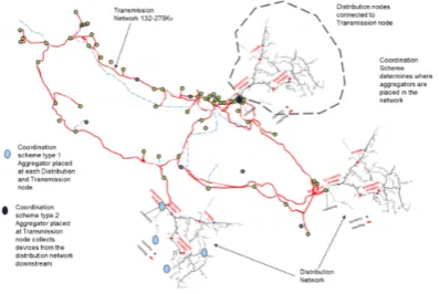
which are scenario driven, determine where the aggregators are placed (Figure 1).
Figure 1: Aggregators assigned to transmission or distribution nodes.
Data for each device and node locations are stored in a Django based SQL database (Django Software Foundation, 2017).
In the current version, buckets are clustered by cost, but the concept can be extended to a more general clustering algorithm using multiple variables.
The CGCL aggregator code makes extensive use of Pythons Numpy Array data manipulation routines for calculation speed, which is ideally suited to n
dimensional matrix manipulation. As illustrated in Figure 2, the CGCL aggregator code is split into two main parts:
CGCL Aggregator Factory. This creates the appropriate number of aggregator agent objects, creates a list (an agent directory) of those objects, so that we can take control of them later and populates them with data from a relational database. On receipt of an aggregation or disaggregation signal from the scheduler module, it also triggers the individual agents to perform their calculations. Currently this is performed sequentially, but this could be multi tasked later. Aggregators are placed at network nodes ;
CGCL Implementation module – that contains the logic of the individual aggregator agents.
Figure 2: CGCL aggregator design.
Control of the aggregator functions is achieved via an external scheduler.
2.2.1
CGCL Aggregator LogicThe aggregator implementation module, contains the logic of the aggregator agents, and currently performs four main tasks:
Initialisation of agent object - When an agent object is created this simple function creates internal storage of variables and sets up parameters such as agent name and ID, max number of bids allowed, device lists and ID’s, the actor that “owns” the aggregator and initialises the arrays for use in the calculations;
Initialisation of agent data - This function pulls device specific data from the database and creates device profiles for the devices attached to the aggregator;
Aggregation – Creates bids for the aggregator and sends these bids to a database, so that the market layers can clear the market;
Disaggregation – Recovers cleared bid data associated with the specific aggregator agent and disaggregates cleared bids. This results in an agent sending new set points to all of the devices on the particular node. These setpoints are stored in an aggregator setpoint out table.
[image:4.595.80.279.128.261.2]buckets or segments and effectively bids this data to the market by storing those bids into an agreed format into database tables.
[image:5.595.335.507.131.225.2]The aggregator sends out forward flexible bids e.g. for the next hour we will bid 12 x 5 minute time intervals. For each time slice, the aggregator sends out bid buckets, which represents the aggregation of all the devices associated with that aggregator. Each bucket represents a price range. E.g. 10-30, 30-70 €/Mwh and so on (see Figure 3).
Figure 3: Bid structure overview.
Each aggregator agent performs its own calculations and updates databases as necessary. A minimum bid size of 1kW is used to filter bid buckets (this is parameter driven).
Bids for the time slices are stored in a 3D array within the agent (flex up and down versions). The matrix represents the clusters/segments as well as the devices in that cluster including details on its type, volumes (real power P and reactive power Q), its bid (price) and so on. This matrix approach allows the logic in the module to unpick cleared bids, disaggregate, and apportion them to individual devices associated with aggregator. We need some way of assigning devices to clusters and to keep a record of it – but at speed. A database solution would have been slow for this purpose.
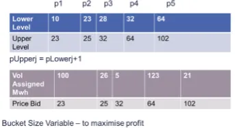
2.3 Agent Aggregation
In the initial design, the aggregator calculated the bucket price ranges so that equal number of devices will be apportioned to each range. The price ranges are therefore variable (see Figure 4). Our current methodology uses a genetic algorithm optimizer to maximise the profit of the aggregator by adjusting the bucket sizes for both the flex up and down bids. Devices are assigned to these buckets based on their
cost, while their ID’s are also stored in tables linked to these buckets.
Figure 4: Bid buckets example.
2.4 Agent Disaggregation
The market is cleared using an OPF calculation. The clearing module then informs aggregators and their schedulers, which trigger the aggregator disaggregation routine. The disaggregator function retrieves accepted bid data from appropriate database table and uses the previously internally stored 3D Numpy arrays (matrices) to unpick the bids to apportion them to individual devices. Where the market clears or accepts the full volume of a particular bucket or segment, the module logic accepts all bids from all the devices assigned to that particular bucket. In the case where the market accepts a fraction of the bid segment, volumes are apportioned on a “greedy” basis – lowest device cost first. Cleared volumes are assigned to individual devices appropriately bucket by bucket, by writing to a setpoint table in the database.
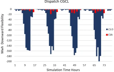
2.5 Simulation Results
[image:5.595.76.283.250.359.2]Figure 5: Volume output for 80 hours of simulation
Figure 6: Price output for 80 hours of simulation.
3
CHALLENGES AND LESSONS
LEARNED
Development of the full SmartNet project has taken many man-years with the CGCL aggregator agent model part taking around 6 man months of effort. Simulation and testing of such a large simulation system is challenging, and we have shown that it is possible to simulate the aggregation and clustering of different types of flexibility into a number of manageable bids. Simulation for 96-time steps on a representation of the Italian grid with 5 types of aggregators using this framework is currently taking around 5-6 hours per scenario using one machine (Alienware 15 R3 7700 HQ 2.8 GHz 4 cores 8 logical 32GB DDR4). Most of the time is spent writing to a single database, which is required to store data on bids and other data for later analysis.
3.1 Database Speed
Simulation write speeds at each tick are shown in Figure 7. The initial design resulted in a single time step write time of around 4 hours at the 40th tick. Optimisation of code using “SQL BulkCreate” commands resulted in a significant drop to around
4-5 minutes. Long write times are a natural consequence of writing around 5 million records per time step.
Figure 7: Database speed during each tick.
Experiments with database writes indicate that having a database index causes the slowdown in insert speed as table size. Removal of the index before writing can improve this performance (Figure 7). Note that indexing does help in improving read speed. A deindexing, write and re-index approach may be worth investigating.
Use of an in-memory database (Anikin, 2016) could also be an option with a “write at leisure” approach to a main database which would be stored on a Hard Disk Drive (HDD). This would be about 200 times faster than the HDD. Our agent design already uses this approach extensively but requires large amounts of memory. Finally, use of a Solid-State Drive (SDD) would bring a speed improvement of around two times over an HDD. We are currently using HDD for storage.
3.1.1 Database Shards
Writing to smaller focussed databases would also help to improve database write performance. SmartNet currently uses one database to store everything. Writing bids to a database for one time period only, “a current time bid database”, could potentially improve performance. Joining of these current bids to a historical collection of bid data could be performed at a later time. We may wish to consider horizontal partitioning of the database or “sharding” (Kerstiens, 2018), although this technique can prove to be slow when querying multiple databases.
3.2 Python Vs Java Vs C++
[image:6.595.75.284.255.364.2]of the order of 100-1000 times, depending on operation, over iterating through a list.
We have considered a port of the code to Java, as it is known that Java code could be up to 50 times faster than python (Gouy, 2018). Benchmarks can range from no speed up for simple algorithms to 50 times or more where computations are complex. Unfortunately, this would involve a large conversion effort and the Python development environment is more productive potentially by a factor of five. A C++ formulation would also provide significant speed improvements over Java and Python but as we have discussed in section 3.1, database operations impose a significant speed restriction on this implementation, which far exceeds any benefit from a swap of language.
Installation of Intel’s ® Python Interpreter using uses its Data Analytics Acceleration and Claim Math Kernel Library could also improve calculation times (Intel, 2018).
3.3 Multi-threading/HPC/CUDA
Multi-threading or the use of a High Performance Computing (HPC) environment could bring significant benefits to simulation times. In a practical sense, each aggregator company in the real world would be aggregating on a separate computer system/server remotely from the TSO/DSO clearing entity. However, HPC data transfer latency could reduce the benefits if machines are located on distant clusters or are at different company premises.
Multithreading allows for improvements in calculation times of the order of 7x (with 8 logical cores) i.e. of the order of 87% x the number of cores. HPC using 65 cores would therefore drastically reduce calculation times to 1-2% of the one machine calculation time if we ignore latency effects. An aggregator with 300,000 devices is taking around 15 secs to perform its calculations on one machine using single threading so a HPC setup could reduce this to around 0.3 secs. An aggregator with a single device is taking around <0.05 secs on a single thread.
Use of a Graphics Processing unit (GPU) with CUDA (Couturier, 2013) would be an ideal method to use on an aggregator module that makes extensive use of the Numpy arrays and associated calculations. We have estimated that speed improvements of around 30X could be made for our design based on the calculations alone when using an Nvidia Geforce GTX 1070 GPU. Database access issues would remain. Speedup will depend on array size, so in the case of very large arrays, we may expect improvement of 100-200, but some of aggregator
arrays only contain 1 device, so the overhead of transferring data to the associated GPU may actually degrade performance. This of course will depend on the number of cores available in the GPU.
3.4 Congestion
Unintended aggregator actions caused DSO agent intervention in the market to relieve network congestion (power flows, voltages). Forecasting errors (day ahead vs real time) also play a part in this process especially when devices promised to deliver more they actually could.
DSO Congestion management has implications for both the overall system costs and aggregator profit margins, and presents additional risks to the aggregator. If the additional risk is high, aggregators may want to anticipate congestion separately from the DSO, and incorporate congestion risk value into their bids.
4
FUTURE WORK
Realistic aspects of aggregation such as risk management, strategic bidding, agent learning, congestion and portfolio management are missing from the current approach. A more realistic representation of a power aggregator will require that we include these various elements. Early work indicates that the price of particular bids could rise by as much as 30% under certain scenarios if we include some of these effects. Finally, the current SmartNet framework does not consider aggregator-to-aggregator interactions nor does it consider aggregators with multiple device types e.g. CGCL + CHP or competition between them. Future versions of our modelling will include this and will implement the mechanisms discussed in section 3.
5
CONCLUSIONS
ACKNOWLEDGEMENTS
This research is funded by the UK Engineering and Physical Science Research Council (EPSRC) and the International Strategic Partner (ISP) Research Studentship and the EU Hor2020 SmartNet project.
REFERENCES
Anikin, D. 2016-10-12 2016. What an in-memory database is and how it persists data efficiently. Available from: https://medium.com/@denisanikin/what- an-in-memory-database-is-and-how-it-persists-data-efficiently-f43868cff4c1.
Couturier, R. 2013. Introduction to CUDA. Designing Scientific Applications on GPUs, 13.
Django Software Foundation 2017. Django Documentation.
Dzamarija, M., Plecas, M., Jimeno, J. & Marthinsen, H. 2018. Aggregation models.
Furlonge, H. I. 2011. A stochastic optimisation framework for analysing economic returns and risk distribution in the LNG business. International Journal of Energy Sector Management, 5, 471-493.
Gouy, I. 2018. Python 3 vs Java - Which programs are faster? | Available: https://benchmarksgame-team.pages.debian.net/benchmarksgame/faster/p ython.html [Accessed].
Intel 2018. Intel® Distribution for Python* Accelerate Python* Performance.
Kerstiens, C. 2018. Database sharding explained in plain
English. Available: https://www.citusdata.com/blog/2018/01/10/shar
ding-in-plain-english/.
Kohansal, M. & Mohsenian-Rad, H. 2016. A closer look at demand bids in california iso energy market. IEEE Transactions on Power Systems, 31, 3330-3331.
Krink, T., Paterlini, S. & Resti, A. 2008. The optimal structure of PD buckets. Journal of Banking & Finance, 32, 2275-2286.
Kumar, D. 2017. The four bucket system. Available: http://vro.in/s33527.
Li, C. 2015. Chance-constraint method - optimization
[Online]. Available: https://optimization.mccormick.northwestern.ed
u/index.php/Chance-constraint_method [Accessed].
Marthinsen, H., Plecas, M., Morch, A. Z., Kockar, I. &
Džamarija, M. 2017. Aggregation model for
curtailable generation and sheddable loads.
Migliavacca, G., Rossi, M., Six, D., Džamarija, M.,
Horsmanheimo, S., Madina, C., Kockar, I. & Morales, J. M. 2017. SmartNet: H2020 project analysing TSO–DSO interaction to enable ancillary services provision from distribution networks. CIRED-Open Access Proceedings Journal, 2017, 1998-2002.
Riskviews. 2012. Five Buckets of Risk. Available: https://riskviews.wordpress.com/2012/01/17/five -buckets-of-risk/ [Accessed 2012-01-17]. Shafie-Khah, M., Heydarian-Forushani, E., Golshan, M.,
Siano, P., Moghaddam, M., Sheikh-El-Eslami, M. & Catalão, J. 2016. Optimal trading of plug-in electric vehicle aggregation agents plug-in a market environment for sustainability. Applied Energy, 162, 601-612.