Performance Optimization of Wireless Sensor Networks

(1)

UC Irvine

UC Irvine Electronic Theses and Dissertations

Title

Performance Optimization of Wireless Sensor Networks Permalink https://escholarship.org/uc/item/9cx187kt Author GUO, JUN Publication Date 2019 Peer reviewed|Thesis/dissertation

(2)

UNIVERSITY OF CALIFORNIA, IRVINE

Performance Optimization of Wireless Sensor Networks DISSERTATION

submitted in partial satisfaction of the requirements for the degree of

DOCTOR OF PHILOSOPHY in Electrical Engineering

by

Jun Guo

Dissertation Committee: Professor Hamid Jafarkhani, Chair Professor A. Lee Swindlehurst Professor Ahmed Eltawil

(3)

c

(4)

LIST OF FIGURES

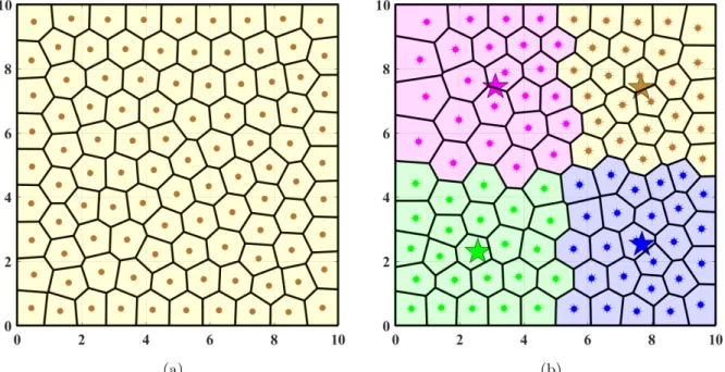
Page 1.1 Two example node deployments. (a) One-tier network. (b) Two-tier network. 100

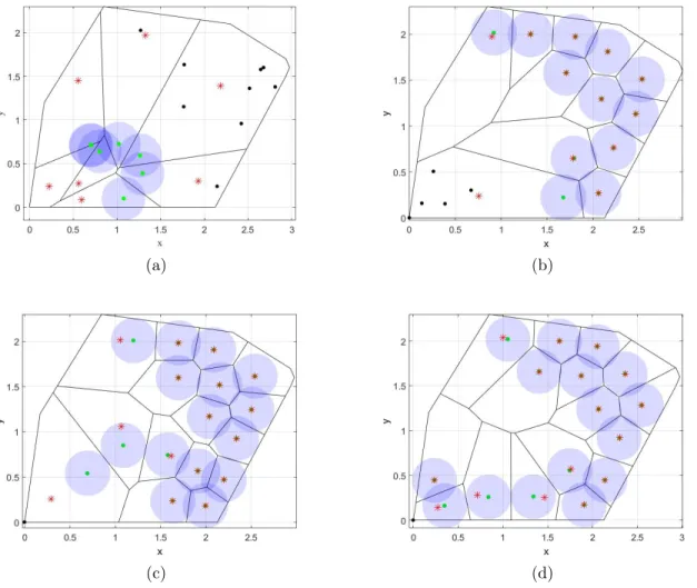
first-tier nodes and 4 second-tier nodes are denoted by dots and stars, respectively. The cell partitions are denoted by polygons. The symbols associated with the same second-tier node are filled with the same color. . . 5 2.1 A non-starshaped desired region. . . 26 2.2 Sensor deployments in WSN1. (a) The initial sensor deployment and the

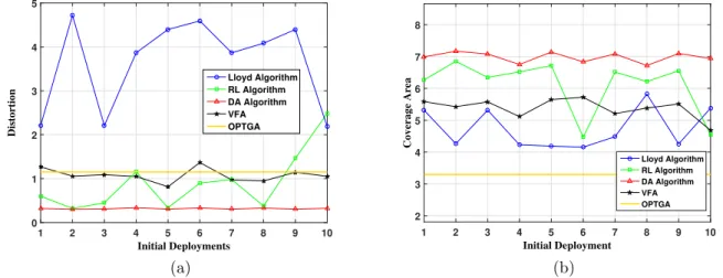
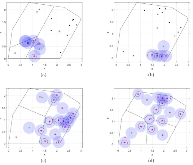
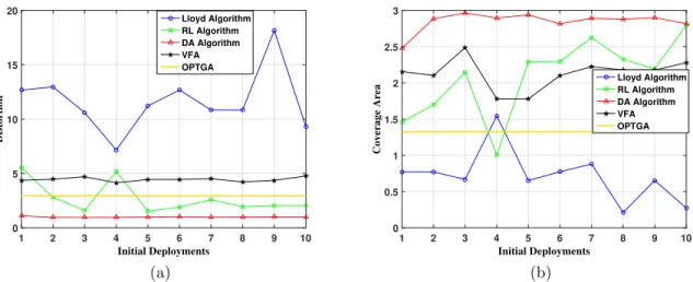
corresponding Voronoi regions. (b) The final deployment of Lloyd Algorithm. (c) The final deployment of RL Algorithm. (d) The final deployment of DA Algorithm. . . 31 2.3 Comparison of performance in WSN1. (a) Comparison of distortion for

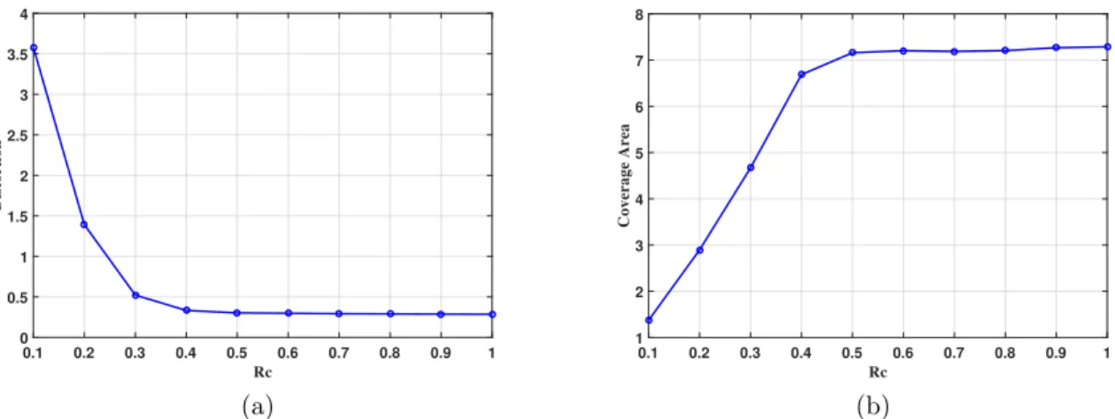
dif-ferent algorithms in WSN1. (b) Comparison of coverage area for difdif-ferent algorithms in WSN1. . . 33 2.4 Relationship between performance andRcin WSN1. (a) Relationship between

distortion andRcin WSN1. (b) Relationship between coverage andRcin WSN1. 34

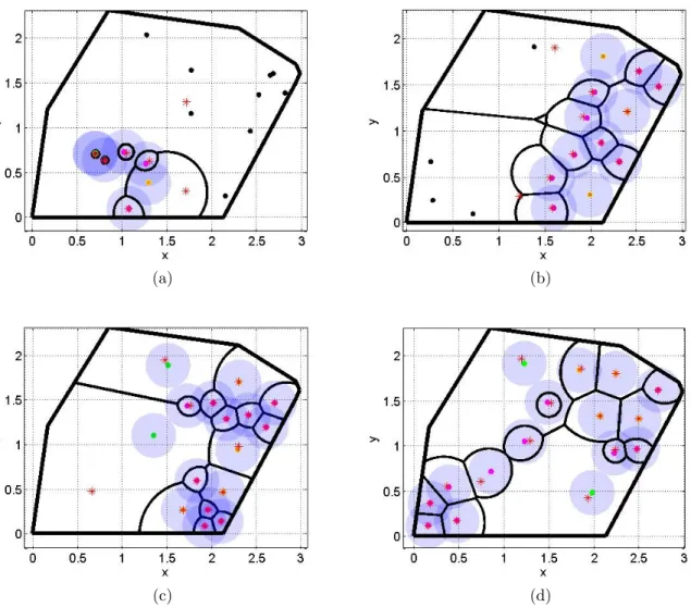
2.5 Sensor deployments in WSN2. (a) The initial sensor deployment and the corresponding weighted Voronoi regions. (b) The final deployment of Lloyd Algorithm. (c) The final deployment of RL Algorithm. (d) The final deploy-ment of DA Algorithm. . . 35 2.6 Sensor deployments in WSN3. Figure (a) The initial deployment and

corre-sponding weighted Voronoi regions. (b) The final deployment of Lloyd Algo-rithm. (c) The final deployment of RL AlgoAlgo-rithm. (d) The final deployment of DA Algorithm. . . 36 2.7 Comparison of performance in WSN2. (a) Comparison of distortion for

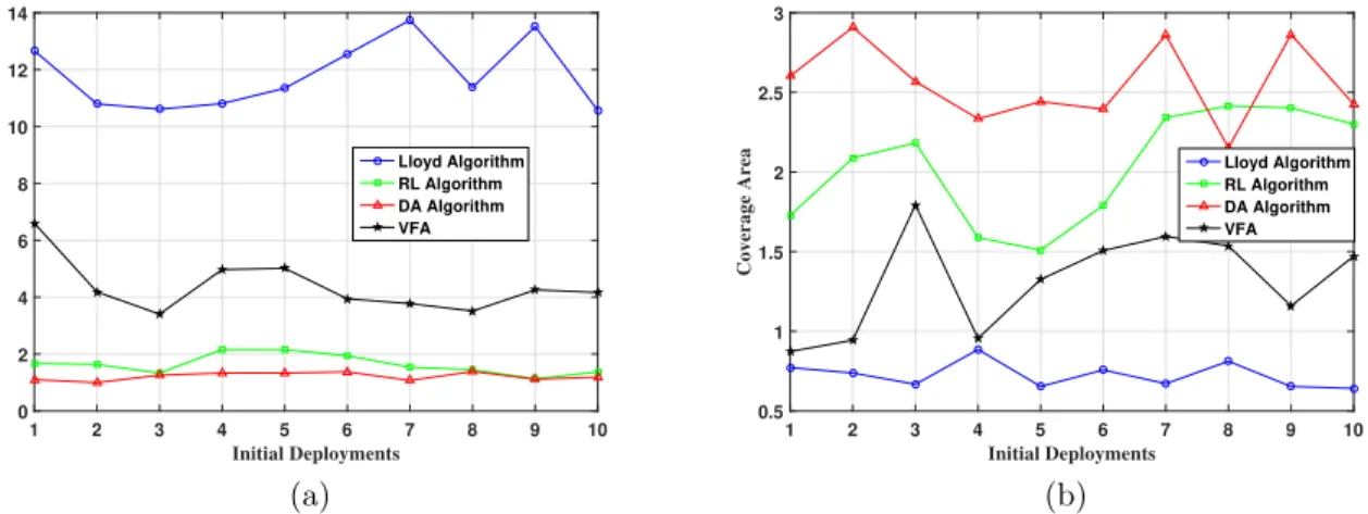
differ-ent algorithms in WSN2. (b) Comparison of coverage for differdiffer-ent algorithms in WSN2. . . 37 2.8 Comparison of performance in WSN3. (a) Comparison of distortion for

dif-ferent algorithms in WSN3. (b) Comparison of coverage area for difdif-ferent algorithms in WSN3. . . 37 2.9 Sensor deployments in WSN2. (a) The initial sensor deployment and the

corresponding weighted Voronoi regions. (b) The final deployment of Lloyd Algorithm. (c) The final deployment of RL Algorithm. (d) The final deploy-ment of DA Algorithm. Two obstacles are shown by the gray region. . . 38

(8)

2.10 Comparison of performance in WSN2. (a) Comparison of distortion for differ-ent algorithms in WSN2. (b) Comparison of coverage for differdiffer-ent algorithms in WSN2. . . 39 3.1 UAV deployment with directed antenna beam and associated GT cells for

α= 2 and N = 2 for a uniform GT distribution. . . 43 3.2 Optimal height (solid) with bound (dashed) and average distortion (dotted) for

N = 2, A= 1 and uniform GT density. . . 52 3.3 Optimal UAV deployment in one dimension for A= 1,α = 1 and N = 2,4 over a

uniform GT density by (3.29). . . 52 3.4 The performance comparison of Lloyd-A, Lloyd-B and Random Deployment

(RD). (a) Uniform density. (b) Non-uniform density. . . 52 3.5 The UAV projections on the ground with generalized Voronoi Diagrams where

α= 2 and the source distribution is uniform. (a) 32 UAVs. (b) 100 UAVs. . 53 3.6 The UAV projections on the ground with generalized Voronoi Diagrams where

α= 2 and the source distribution is non-uniform. (a) 32 UAVs. (b) 100 UAVs. 54 4.1 Two deployment examples in a 1-dimensional space with one FC. (a) The

AC/DC two-tier quantizer. (b) The optimal quantizer. AP and FC locations are denoted by circles and star. The optimal partition cells are denoted by intervals. Each AP and its corresponding cell are illustrated by the same color. 61 4.2 Two deployment examples in a 1-dimensional space with two FCs. (a) The

AC/DC two-tier quantizer. (b) The optimal two-tier quantizer. AP and FC locations are denoted by circles and stars. The optimal partition cells are denoted by intervals. Each AP and its corresponding cell are illustrated by the same color. The two clusters are denoted by solid and dashed lines. . . . 65 4.3 AP and FC deployments of different algorithms in WSN1. (a) MER. (b) AC

(c) DC. (d) CL. . . 74 4.4 AP and FC deployments of different algorithms in WSN2. (a) MER. (b) AC

(c) DC. (d) CL. . . 75 4.5 The weighted power comparison of different Algorithms. (a) WSN1. (b) WSN2. 76 4.6 The comparison between the AP-Sensor power function and the performance

of TTL: (a) One-dimensional region uniformly distributed in [0,1]. (b) WSN1. 77 5.1 Example1: (a) DR and FR for Sensor 1; (b) ADR and AFR for Sensor 1;

(c) SDR and SFR for Sensor 1; DR, ADR, and SDR are shown by green. FR, AFR, and SFR are shown by the intersections of green regions and the magenta circles. Communication ranges, movement range, and Connections are, respectively, denoted by black doted curves, magenta solid curve, and red lines. . . 84

(9)

5.2 Centralized sensor deployments: (a) VFA in MWSN1; (b) Lloyd-αin MWSN1; (c) CCML in MWSN1; (d) VFA in MWSN2; (e) Lloyd-α in MWSN2; (f) BCCML in MWSN2. The initial sensor locations are denoted by green dots. The final locations of active and inactive sensors are denoted by red and black dots. The sensing regions of active and inactive sensors are denoted by blue and black. The movement paths are denoted by blue lines. . . 100 5.3 Performance comparison for centralized sensor deployment. (a) Distortion in

MWSN1; (b) Distortion in MWSN2; (c) Area coverage in MWSN1; (d) Area coverage in MWSN2. . . 101 5.4 Distributed sensor deployments: (a) VFA in MWSN1; (b) Lloyd-αin MWSN1;

(c) DCML in MWSN1; (d) VFA in MWSN2; (e) Lloyd-α in MWSN2; (f) DCML in MWSN2. The initial sensor locations are denoted by green dots. The final locations of active and inactive sensors are denoted by red and black dots. The sensing regions of active and inactive sensors are denoted by blue and black. The movement paths are denoted by blue lines. . . 102 5.5 Performance comparison for distributed sensor deployment. (a) Distortion in

MWSN1; (b) Distortion in MWSN2; (c) Area coverage in MWSN1; (d) Area coverage in MWSN2. . . 104 5.6 The target coverage in MWSN1. (a) Basic+ECST-H; (b)

TV-Greedy+ECST-H; (c) CCML. The covered targets and uncovered targets are denoted by magenta triangles and black triangles, respectively. . . 105 5.7 The target coverage in MWSN1. (a) Rc = 0.4, Rs = 0.2; (b) Rc = 0.5,

Rs = 0.25. The target coverage of Basic+ECST-H, TV-Greedy+ECST-H,

(10)

LIST OF TABLES

Page 2.1 Simulation Parameters of Static Wireless Sensor Networks . . . 31 2.2 Distortion Comparison (µ: the average distortion,σ: the standard deviation) 37 4.1 Running times(s) . . . 76 5.1 Simulation Parameters of Mobile Wireless Sensor Networks . . . 98

(11)

LIST OF ALGORITHMS

Page 1 Restrained Lloyd Algorithm . . . 27 2 Deterministic Annealing Algorithm . . . 30 3 Centralized Constrained Movement Lloyd Algorithm . . . 87 4 Backwards-stepwise Centralized Constrained Movement Lloyd Algorithm . . 89 5 Distributed Constrained-Movement Lloyd Algorithm . . . 94

(12)

ACKNOWLEDGMENTS

First, I would like to thank my advisor Prof. Hamid Jafarkhani for the continuous support of my Ph.D. study and related research. His professional and patient guidance helped me in aspect of learning, research and writing, including this dissertation. In addition, Professor Hamid Jafarkhani inspired my interests and willpower by posting weekly motto attachment on his door.

Besides my advisor, I am also grateful to my parents, who have provided me with moral and emotional support throughout my years of study and as well as process of researching and writing this thesis. Moreover, I acknowledge my other family members and friends who have supported me along the way. This accomplishment would not have been possible without them.

Another very special gratitude goes out to DARPA’s GRAPHS Program, National Science Foundation, and also Holmes Foundation for providing funding for my research. I must ex-press my very profound gratitude to Institute of Electrical and Electronics Engineers (IEEE) for offering me the permissions to incorporate my previous works into this dissertation. And finally, graditude goes to everyone in the Center for Pervasive Communications and Computing (CPCC); it was great sharing laboratory with all of you during the last four and a half years. With a special mention to Erdem Koyuncu, Philipp Walk, and Saeed Karimi Bidhendi, it was extremely impressive to have the opportunity to collaborate with you for the majority of my research in the past several years.

(13)

CURRICULUM VITAE

Jun Guo

EDUCATION

Doctor of Philosophy in Electrical Engineering 2014 – 2019

University of California, Irvine Irvine, USA

Master in Electrical Engineering 2011 – 2014

Beijing University of Posts and Telecommunications Beijing, China

Bachelor of Science in Electrical Engineering 2007 – 2011

RESEARCH EXPERIENCE

Graduate Research Assistant 2014 – 2019

University of California, Irvine Irvine, USA

TEACHING EXPERIENCE

Teaching Assistant 2011 – 2014

WORKING EXPERIENCE

Data Engineer Intern Jun. 2018 – Sept. 2018

Amazon Corporation San Francisco, USA

Software Developer Engineer Intern Jun. 2017 – Sept. 2017

Amazon Corporation San Francisco, USA

Research Intern Dec. 2012 – Dec. 2013

(14)

REFEREED JOURNAL PUBLICATIONS

Sensor Deployment with Limited Communication

Range in Homogeneous and Heterogeneous Wireless Sensor Networks

Oct 2016

IEEE Transactions on Wireless Communications vol. 15, no. 10, pp. 6771-6784

A source coding perspective on node deployment in two-tier networks

Jul 2018 IEEE Transactions on Communications

vol. 66, no. 7, pp. 3035-3049

Movement-efficient Sensor Deployment in Wireless Sen-sor Networks with Limited Communication Range

Jan 2019 IEEE Transactions on Wireless Communications

revision is under review

Optimal deployment of UAVs equipped with directional antennas

Feb 2019 in preparation

REFEREED CONFERENCE PUBLICATIONS

Sensor Deployment in Heterogeneous Wireless Sensor Networks

Dec 2016 IEEE Global Communications Conference (Globecom)

Energy efficiency in two-tiered wireless sensor networks May 2017

IEEE International Conference on Communications (ICC) Movement-efficient Sensor Deployment in Wireless Sen-sor Networks

May 2018 IEEE International Conference on Communications (ICC)

Quantizers with Parameterized Distortion Measures Mar 2019

IEEE Data Compression Conference (DCC)

Using Quantization to Deploy Heterogeneous Nodes in Two-Tier Wireless Sensor Networks

Jul 2019 IEEE International Symposium on Information Theory (ISIT)

submitted

Energy Efficient Node Deployment in Wireless Ad-hoc Sensor Networks

Dec 2019 IEEE Global Communications Conference (Globecom)

(15)

ABSTRACT OF THE DISSERTATION

Performance Optimization of Wireless Sensor Networks By

Jun Guo

Doctor of Philosophy in Electrical Engineering University of California, Irvine, 2019

Professor Hamid Jafarkhani, Chair

In this dissertation, I study three factors, sensing quality, connectivity, and energy con-sumption in static/dynamic wireless sensor networks (WSNs). First, taking sensing quality and connectivity into account, I formulate the node deployment problem in both WSNs from a source coding perspective. According to our analysis, the techniques in regular quantizer can be applied to both homogeneous and heterogeneous WSNs. Second, a one-tier quantizer with parameterized distortion measures is proposed for 3-dimension node deployment prob-lems. Similarly, a novel two-tier quantizer, which can be applied to energy conservation in two-tier WSNs consisting of N access points and M fusion centers, is appropriately defined and studied. In addition, to make a trade-off between sensing quality and communication energy consumption within static WSNs, routing algorithms are appropriately taken into the system model. Moreover, a comprehensive optimization problem is provided to pro-cess all three factors in a dynamic WSN where movement energy dominates total energy consumption. The necessary conditions for the optimal solutions in the above performance optimization problems are proposed in this dissertation. Based on these necessary conditions, a series of Lloyd-like algorithms are designed and implemented to optimize the performance in different WSNs. My experiment results show that the proposed algorithms outperform the existing algorithms in the corresponding WSNs.

(16)

Chapter 1 Introduction

1.1 Background

As a bridge between the physical world and the virtual information word, wireless sensor networks (WSNs) collect data from the physical world and communicate it with the virtual information world, such as computers. On the one hand, from the perspective of mobility, sensors can be classified as static sensors and mobile sensors [1]. Static sensors, such as temperature sensors, stay still after their one-time deployment while mobile sensors, such as robots and unmanned aerial vehicles (UAVs), are equipped with motion components and able to move to other locations. On the other hand, according to sensors’ functionality/capacity, WSNs can be classified into homogeneous WSNs and heterogeneous WSNs. In homogeneous WSNs, extensively studied in the literature [2]–[31], sensors share the same capacity, e.g., storage, computation power, sensitivity, communication radius, coverage radius, moving ef-ficiency, and battery. The heterogeneous WSNs consist of sensors with different capacities [32]–[38]. Proper sensor deployment improves monitoring and controlling of the physical en-vironment, such as temperature, humidity, voice and so on. To accomplish their tasks, WSNs

(17)

should address three needs: (i) Sensing in the target region and (ii) network connectivity, and (iii) energy conservation.

One major challenge in both homogeneous and heterogeneous WSNs is the deployment of nodes to improve the sensing quality. To evaluate the sensing quality, the binary coverage model [2]–[9], [11], [12], [32], [33], [36], [39]–[45] and the probabilistic model [46]–[51] are widely used in WSNs. In the binary coverage model, sensors can only detect the points within a range ofRs. The rangeRsis called the sensing range. In the probabilistic coverage

model, the probability that a sensor detects an event depends on the distance between them. When the number of sensors is large enough to cover the whole sensing region, the coverage degree in [11], [52] is used to evaluate sensing performance. On the contrary, when the sensing region is too large to be covered by the given sensors, the coverage area is used as the performance measurement [36]. There are many coverage models and deployment algorithms, for different sensing tasks, in the literature; look at [2]–[4] and the references therein. According to the sensing tasks, coverage models can be classified into four popular categories: (i) area coverage, (ii) target coverage, (iii) barrier coverage, and (iv) sensing uncertainty. A natural sensing task is to maximize the area coverage, which is formulated by the total area covered by sensors. In another popular coverage model, target coverage, the specific target locations are detected and reported by relocated sensors. In this case, sensors or robots are required to collect detailed information from discrete targets. A full-target-coverage is achieved if and only if every discrete target in the 2-dimensional region is covered by at least one sensor. Sensors in barrier coverage model move along the boundary to detect intruders as they cross the border of a region or domain. To obtain full-barrier-coverage, one should place sensors to cover the whole barrier or boundary. Finally, the minimization of sensing uncertainty requires sensors to form a Centroidal Voronoi Tessellation (CVT). It is mainly used when there is no specific target. The widely used sensing uncertainty model can be presented as a quantizer with the sensing uncertainty as its distortion [2]–[10], [13], [15]–[18], [32]–[34], [53]–[55]. In fact, WSNs should be reconfigurable/flexible to support

(18)

different sensing tasks. However, to the best of our knowledge, there is no unified framework that models a variety of coverage tasks.

Connectivity is another important requirement in WSNs. In WSNs, mobile sensor nodes are relocated to collect physical information, such as magnetism, temperature, and voice. The collected data is forwarded to the outside world through access points (APs). Therefore, the collected data is useless if it cannot be forwarded to the AP via single-hop or multiple-hop communications. When sensors are connected by wirelines, the connectivity is guaranteed automatically. The connectivity is still a challenge in WSNs where sensors are communicating with each other through wireless channels. A common communication model [3], [6], [10]– [12], [14], [52] assumes that each sensor node is able to communicate with sensors in a limited communication rangeRc. The Critical Sensor Density (CSD) [3] is the number of nodes per

unit area required to provide full coverage when the communication range is limited.

Energy efficiency is another key issue in WSNs, as most sensors have limited battery energy, and it is inconvenient or even infeasible to replenish batteries of numerous densely deployed sensors [18]. In general, the energy consumption of a device includes communication energy, data processing energy [56], sensing energy, and movement energy. In fact, sensor movement has a much higher level of energy consumption compared to other types of energy [19], [20]. Except movement, wireless communication is the primary source of energy consumption. Therefore, movement energy and communication energy will dominate the energy consump-tion in static WSNs and mobile WSNs, respectively. Literature [57] studies the optimal angular velocity and the optimal acceleration to minimize the energy consumption for mo-tion. Simulation results in [57] show that the energy consumption for one-step motion with the optimal angular velocity setting is approximately linear to the movement distance. In fact, the linear movement energy consumption is a popular assumption and widely adopted in the literature [21]–[23], [35], [58]. Particularly, the movement energy consumption in some specific sensors is 5.976J/m [58]. Total energy consumption and network lifetime are two

(19)

common energy-related measures. When battery charging is available, total energy mini-mization is an important issue in WSNs. Otherwise, network lifetime maximini-mization, which balances the energy consumption among sensors, is a more common and challenging problem because it takes into account the available battery power of sensors.

1.2 Node deployment from a source coding perspective

1.2.1 One-Tier Quantization for Node Deployment

In many applications, one needs to provide service to and collect data from a geographical area of interest via multiple nodes, such as sensors or providers. Usually, the nodes are distributed such that each point or client in the area is only served by only one node, resulting in a partition of the target area to disjoint regions. The service cost for each node may depend on its characteristics and local service region. The fundamental goal in such a formulation is to jointly optimize the node locations and the corresponding service regions to optimize the overall performance, which is typically defined as an aggregate of node service costs.

The cost of providing service to a client is usually related to its distance to the local service node. Therefore, minimizing the total cost by optimally deploying the nodes and the service regions is identical to a spatial tessellation problem [33]. Such problems (which have also been referred to as facility location or node deployment problems by different research com-munities) are equivalent to the quantization problem of data compression and source coding. In fact, in the language of quantization theory, the service nodes and service regions cor-respond to the reproduction points and quantization regions, respectively. Minimizing the total service cost becomes equivalent to minimizing the corresponding average distortion. We now present several specific applications to highlight the above equivalency.

(20)

In sensor networks, sensors are deployed in a two-dimensional planar to collect data from the environment. The goal of sensor/node deployment is to maximize the sensing performance and quality. An example of the sensor deployment in a two-dimensional planar is illustrated

(a) (b)

Figure 1.1: Two example node deployments. (a) One-tier network. (b) Two-tier network. 100 first-tier nodes and 4 second-first-tier nodes are denoted by dots and stars, respectively. The cell partitions are denoted by polygons. The symbols associated with the same second-tier node are filled with the same color.

in Fig. 1.1a, where each sensor is denoted by a dot that monitors its own region. In this scenario, the reproduction points correspond to the sensor nodes, and the quantization Voronoi regions correspond to the sensor partitions. The cost function (distortion measure) is usually a monotonically increasing function of the distance between the sensor and the event that is being sensed, and quantifies the inaccuracy of sensing. The most common cost function used in the quantization literature is the squared Euclidean distance [59]. It can be used directly in the sensor network example to measure the overall sensing inaccuracy in homogeneous wireless sensor networks (WSNs) [6]. For heterogeneous WSNs, a weighted Euclidean distance square measure can be used where the weights reflect the nodes’ different sensing capabilities [32]. Other cost functions have also been utilized to formulate the sensing coverage or the sensing probability [32], [47], [60], [61].

(21)

networks where user equipments (UEs) are considered as the source, heterogeneous BSs are recognized by the reproduction points, and the BS cells are represented by the quantization Voronoi regions. Because of the path loss, the signal strength at the receiver is a non-increasing function of the communication distance [65]–[67]. Using such a non-non-increasing function as the cost function, the distortion measure can be defined as the expected signal to noise ratio (SNR) at the UEs, where the expectation is calculated for a given channel probability distribution.

1.2.2 Two-Tier Quantization for Node Deployment

The conventional spatial tessellation and node deployment problems in Section 1.2.1 ignore the hierarchical architecture that is inherent in many networks. In fact, to reduce the network burden, many practical networks have a two-tier structure, as an extension to the one-tier examples considered in Section 1.2.1. For example, to provide an effective delivery service for the residents, the postal system uses a two-tier network including the local post offices and the postal hubs. Then, there will be two costs associated with each delivery. Afirst-tier-cost

that is the cost of delivering packages from clients to local post offices, determined by the population density and the distance from clients to their local post offices, and a

second-tier-cost which is the total cost of delivering packages between local post offices and the

corresponding postal hubs. The second-tier-cost is determined by the workload of the local post offices and the distance from the local post offices to their postal hubs. A similar two-tier network appears in the hospital system where local hospitals provide the basic medical treatment and the residents with severe disastrous issues are transferred to the hospital centers with more medical facilities.

Two-tier WSNs and two-tier cellular networks are also very common network architectures. A two-tier WSN [37], [38], [68]–[70] includes densely deployed sensors, multiple access points (APs), and fusion centers (FCs). In such a network, sensor nodes collect the data and send it to their APs for processing. Then, each AP transmits its aggregated data to its associated

(22)

FC [37], [38], [68]–[70]. As depicted in Fig. 1.1b, the sensors, APs, and FCs correspond, respectively, to clients, first-tier nodes, and second-tier nodes in our two-tier network. One reasonable cost function in the two-tier WSN is the total energy consumption at sensors and APs. The objective is to optimize the trade-off between the sensor and AP energy consumption.

The goal of this paper is to study node deployment problems in two-tier networks, where two-tier nodes are deployed to provide service for the clients in the target region. In such two-tier networks, as depicted in Fig. 1.1b, the second-tier nodes provide service for the first-tier nodes that serve the clients. Similar to the one-tier networks, the cost between two points is generally a non-decreasing function of the Euclidean distance. Let the first-tier-cost be the total cost between clients and first-tier nodes, and the second-tier-cost be the total cost between the tier nodes and the corresponding second-tier nodes. Moving the first-tier nodes towards the second-first-tier nodes, usually, will increase the average distance between the first-tier nodes and the local clients, resulting in the increase of the first-tier-cost. On the other hand, moving the first-tier nodes towards the local clients, usually, will increase their distance to the second-tier nodes and will result in an increase in thesecond-tier-cost. Therefore, there is a trade-off between the first-tier-cost and the second-tier-cost.

1.3 Related Work

1.3.1 Quantization

A significant body of literature exists on designing the one-tier quantizers. Gray et al. [59] summarize the theory and practice of quantization since its inception. The best possible quantization distortion in a high-resolution regime has been discussed in [71]–[73] and the application of the high-resolution theory to node deployment in heterogeneous sensor net-works is provided in [74]. Clustering is a related method where the cluster heads and cluster regions are, respectively, the reproduction points and quantization regions. Many different

(23)

hierarchical clustering methods, such as Agglomerative Clustering (AC) and Divisive Clus-tering (DC), are discussed in [75]. Furthermore, some existing quantization schemes in the literature can be employed to the two-tiered quantizers. For example, successively refinable vector quantizers (SRVQs) [76]–[78] have multiple stages. As another example, hierarchical vector quantizers (HVQs) [79]–[81] are proposed to reduce the quantizer encoding complexity. HVQs employ quantizers of different dimensions in different hierarchical steps.

1.3.2 Node Deployment

A huge body of literature exists on energy-efficient sensor relocation. However, most of the papers in the literature consider one or two key metrics rather than all the three (sensing quality, connectivity, and energy efficiency) together. Moreover, there is no unified framework that can support different coverage models. References [21]–[23], [35], [36] study the energy saving with a full-area-coverage guarantee. Hungarian Algorithm is applied to minimize the total energy consumption after the full-area-coverage is achieved by Genetic Algorithm [21]. Similarly, the grid-based algorithms are proposed in [82] to reduce the total energy consumption while keeping the full-area-coverage and full-connectivity. Kuei-Ping et al. [83] propose a distributed partition avoidance lazy movement (PALM) protocol, which avoids unnecessary movement, to ensure both full-area-coverage and connectivity. Shuhui et al. [84] provide a scan-based relocation algorithm, SAMRT, which is supposed to be energy-effective with densely deployed sensors. Note that the above method put sensing quality as the first priority, and the energy efficiency is merely the secondary objective. To provide a flexible and fair trade-off between area coverage and energy consumption, virtual force based algorithms, HEAL [22], VFA [23], [36], and DSSA [35], are proposed. In [35], the authors take into account the local sensor density, and thus avoid unnecessary movements in the region with densely deployed sensors. In [22], HEAL is designed to mend area coverage holes while minimizing the moving distance. However, the main assumption that there are enough sensors to achieve full-area-coverage, limits its usage. A virtual force based algorithm, VFA

(24)

[23] is proposed to maximize the area coverage while saving energy. Instead of saving the total energy consumption, another virtual force based algorithm, VFA, is proposed in [23] to prolong the network lifetime during the area coverage maximization. Besides, a variant of VFA is designed in [36] to maximize the area coverage in a heterogeneous WSN. However, connectivity is not considered in [22], [23], [35], [36].

Sensor relocation for target coverage and barrier coverage is also well studied. Rout et al. [24] design a virtual-force based algorithm, OATIDA, to obtain both full-target-coverage and full-connectivity on a region with obstacles, while energy consumption is ignored. Chen et al. [25] propose a two-phase algorithm to achieve full-target-coverage with minimum total energy consumption, but connectivity is not taken in to account. Similarly, Njoya et al. [27] design an evolutionary-based framework to make the trade-off between target coverage and network lifetime while the connectivity issue is ignored. Liao et al. [26] investigate how to deploy mobile sensors with minimum total energy consumption to form a WSN that provides both full-target-coverage and full-connectivity. Although all three factors are considered in [26], full-target-coverage and full-connectivity are implemented sequentially, which requires redundant sensors. On the other hand, the existing literature on barrier coverage also seeks the perfect sensing quality, i.e., full-barrier-coverage. Chen et al. [28] focus on 1-dimensional barriers, and then provide an energy-efficient relocation plan to obtain full-barrier-coverage. In [29], a greedy algorithm with binary search is applied to achieve maximum network lifetime and 2-dimensional full-barrier-coverage simultaneously. A faster algorithm which achieves the same purpose as [29] is provided in [30]. Still, the above sensor relocation algorithms designed for barrier coverage ignore the connectivity requirement.

Even if the entire region, targets, or barriers are covered, sensors have different sensing accuracy at different points in the covered region. In fact, sensing capability diminishes as the distance increases [6], [33], [85]–[92]. Therefore, a distance based model, sensing uncertainty (or CVT model), has also been investigated in the literature. Distortion, as an important parameter in source coding, models the sensing uncertainty via a function

(25)

of distance [2]–[10], [13], [15]–[18], [32]–[34], [53]–[55], [91]. One can minimize distortion in WSNs through vector quantization techniques in [59], [93]. Lloyd algorithm [94] is one of the tools to minimize distortion in WSNs. The convergence of the Lloyd algorithm has been studied in [95]–[97]. Taking both connectivity and sensing uncertainty into account, our previous work [32], [98] proposes the necessary conditions for the optimal sensor relocation in heterogeneous WSNs. Unfortunately, another key metrics, energy consumption, is not taken into consideration. Li et al. [9] explore directional sensors whose sensing uncertainty varies among different directions, and then design two iterative algorithms to optimize the sensor deployment. However, energy consumption is not taken into their objective function. The energy consumption of directional sensors or UAVs are analyzed in my previous work [55]. A natural approach to save energy is to add an energy-related penalty term into the objective function. In [10], the authors propose two Lloyd-like algorithms, Lloyd-α and DEED, to minimize sensing uncertainty with a movement related penalty function. For Lloyd-α, the movement in each iteration is scaled by a parameter α ∈ [0,1]. In DEED, the penalty function is properly selected with a positive definite matrix depending on a parameter δ, and then the movement is optimized with the help of the gradient and Hessian matrix of the distortion. Note that one has to manually adjust the parameter α (or δ) for Lloyd-α

(or DEED) to satisfy a specific energy constraint. To overcome this weakness, two Lloyd-like algorithms without any intermediate parameter are proposed in my previous work [53]. These two algorithms can be employed to minimize sensing uncertainty with a total energy constraint or a network lifetime constraint.

1.4 Contributions and Organization

In this dissertation, I study the performance (sensing quality, connectivity, and energy con-sumption) optimization in WSNs and make the following contributions: (1) The sensing quality in heterogeneous WSNs with limited communication range is formulated as a one-tier

(26)

quantizer. (2) Both theoretical analysis and numerical algorithms are proposed to optimize the sensing quality with the connectivity guarantee. (3) The optimal UAV deployment is found to minimize the the uplink communication energy conservation in 3-Dimension WSN. (4) The energy consumption in a two-tier WSN is formulated as a two-tier quantizer. (5) Based on the necessary conditions, Lloyd-like algorithms are proposed to search the optimal node deployment. (6) A unified optimization framework for different coverage models is pro-vided that takes three key metrics, sensing quality, connectivity, and energy consumption, into consideration. (7) By providing analytical necessary conditions, I design centralized and distributed Lloyd-like algorithms to optimize sensor relocation with (i) network lifetime constraints and (ii) limited communication ranges.

In the rest of this dissertation, I first study the sensing quality in both homogeneous and heterogeneous WSNs with limited communication range in Chapter 2. In Chapter 3, I explore the energy conservation of WSNs with directional UANS. In Chapter 4, I analyze the optimal node deployment and cell partition to minimize the average power in a two-tier WSN. After that, a unified optimization framework for different coverage models is provided in Chapter 5. Finally, I conclude my work in Chapter 6.

(27)

Chapter 2 Sensor Deployment with Limited

Communication Range in

Homogeneous and Heterogeneous

Wireless Sensor Networks

In this chapter, I study the heterogeneous wireless sensor networks (WSNs) and propose the necessary condition of the optimal sensor deployment. Similar to that in homogeneous WSNs, the necessary condition implies that every sensor node location should coincide with the centroid of its own optimal sensing region. Moreover, I discuss the dynamic sensor de-ployment in both homogeneous and heterogeneous WSNs with limited communication range for the sensor nodes. The purpose of sensor deployment is to improve sensing performance, reflected by distortion and coverage. I model the sensor deployment problem as a source cod-ing problem with distortion reflectcod-ing senscod-ing accuracy. However, when the communication range is limited, a WSN is divided into several disconnected sub-graphs under certain con-ditions as I will discuss in this paper. In such a scenario, neither the conventional distortion nor the coverage represents the sensing performance as the collected data in disconnected

(28)

sub-graphs cannot be communicated with the access point. By defining an appropriate sens-ing performance measure, I propose a Restrained Lloyd (RL) algorithm and a Deterministic Annealing (DA) algorithm to optimize sensor deployment in both homogeneous and hetero-geneous WSNs. Our simulation results show that both DA and RL algorithms outperform the existing algorithms when communication range is limited.

2.1 System Model and Problem Formulation

Let Ω be a simple convex polygon in_R2 _{including its interior. Given}_N _{sensors in the target} area Ω, sensor deployment is defined by P = (p1,· · · ,pN) ⊂ ΩN, where pn is Sensor n’s

location. For any pointω ∈Ω,f(ω) is the probability density function of an event at point

ω. I denote the first N natural numbers by [N] ={1, . . . , N}. A cell partition R of Ω is a collection of disjoint subsets of{Rn(P)}n∈[N]whose union is Ω. LetB(c, r) ={ω| kω−ck ≤

r}be a disk centered atcwith radiusrin two-dimensional space. For two pointsaandb, let equationEq+F = 0, where E ∈_R1×2 _{is a 1}_×_{2 matrix and} _F _∈

R is a constant, define the

perpendicular bisector hyperplane between the two points. Then, the equationsEq+F ≥0 and Eq +F ≤ 0 define two half spaces. I denote the half space that contains point a by

HS(a, b).

As mentioned before, I define the AP as the sensor node that can communicate with the outside information world. Let S(P) be the set of sensor nodes that can communicate with the AP when the sensor deployment isP. Note that in general not all nodes can communicate with the AP and card(S(P)) ≤ N, where card(A) is the number of elements in set A. I define a new sensor deployment, which is a subset of the all sensor locations, H(P) as the vector of sensor locations for the card(S(P)) sensor nodes connected to the AP. WhenS(P) includes all sensor nodes, we haveP=H(P) andcard(S(P)) =N. LetU be the set of sensor deployments that provide full connectivity, i.e., U = {P|card(S(P)) = N}. In my model, two sensor nodes can communicate with each other within one hop if and only if the distance

(29)

between the two is smaller than Rc, whereRc is referred to as the communication range. A

sensor node can transfer data outside if and only if there exists a path from the sensor to the AP. The path consists of a sequence of sensor nodes where each hop distance is smaller than the communication rangeRc. Sensor nodes that are connected to the AP construct the

backbone network. Specifically, I can choose the AP as the root and run Breadth First Search (BFS) or Depth First Search (DFS) to obtain the spanning tree. Obviously, sensors in the spanning tree construct the backbone network. If all sensors are included in the backbone network, I call the network fully connected. Otherwise, the network is divided into several disconnected sub-graphs.

Another important factor in analyzing the performance of a WSN is its sensing distance. Sensing performance directly depends on distance [6], [33], [85]–[92]. Therefore, to represent the average sensing accuracy in the target area, I define the following general performance measure: D(P) = N X n=1 Z Rn(P) f(n)(kω−pnk)f(ω)dω, (2.1)

where performance functionf(n)_:

R+ →R+ is a non-increasing function of the distance be-tween pn and ω. When sensors have an identical performance function, i.e., f(n)(·) = f(·),

(2.1) becomes the performance measure in homogeneous WSNs and has been widely used in different applications, such as the precipitation estimation problem in [33]. The parti-tion {Rn(P)}n∈[N] in the above definition include all sensor nodes. However, as explained previously, when the communication range is limited, some sensor nodes cannot transfer their data back to the AP. As a result, only the sensor nodes in the backbone network can contribute to the sensing and therefore the performance should be revised as

D(P) = X

n∈S(P)

Z

Rn(H(P))

f(n)(kω−pnk)f(ω)dω. (2.2)

(30)

only the sensor nodes that are in the backbone network. I reiterate that in the case of a fully connected network, H(P) = P, Eqs. (2.1) and (2.2) are identical. Given a fully connected network, the distortion D(P) = D(P,R(P)) is determined by the sensor deployment P and the cell partition R(P). In homogeneous WSNs, every point should be detected by the nearest sensor in order to make the largest contribution to the total performance. This is because (i) all sensors in homogeneous WSNs have the same performance function f(x) which is only determined by the Euclidean distance x = kω− pnk, and (ii) the sensing

ability diminishes as the distance increases. Therefore, given the sensor deployment, Voronoi partitions [33], [99] provide the optimal performance. The Voronoi partition of Ω generated byP with respect to the Euclidean norm is the collection of sets {Vn(P)}n∈[N] defined by

Vn(P) = {ω∈Ω| kω−pnk ≤ kω−pkk,∀k∈[N]}, (2.3)

where k · kis the Euclidean norm.

However, different sensors with different complexity, power, and sensing ability are used in heterogeneous WSNs. As I will show later, the optimal partitioning in this case is MWVD [44]. The MWVD of Ω generated by Pis the collection of sets VH

n (P)n∈[N] defined by

V_nH(P) = {ω∈Ω| ηnkω−pnk2 ≤ηkkω−pkk2,∀k ∈[N]}, (2.4)

where the cost parameters {ηn ∈ R+}n∈[N] are constants that depend on the sensor char-acteristics, indicating the quality of sensor nodes. For example, the transmission power of Radar sensors, like the distance between the sensor and the events, has a direct influence on the sensing performance [87]. Therefore, radar sensors with different transmitting power will have different sensing abilities. In this case, ηndepends on the transmitting power. The

smaller the cost parameter, the stronger the sensing ability. Both Voronoi regionsVn(P)n∈[N] and MWVDs VH

n (P)n∈[N] are functions of P. Since the Voronoi partitioning can be con-sidered as a special case of the weighted Voronoi partitioning, in which ηn = 1, n ∈ [N], I

(31)

simply use VH

n (P)n∈[N] to represent both. Placing (2.4) back to (2.2), I will have

D(P) = X n∈S(P) Z VH n (H(P)) f(n)(kω−pnk)f(ω)dω. (2.5)

Obviously, choosing different functions f(n)₍_·_{) in (2.5) results in different problem} formula-tions. One natural choice for the functionf(n)₍_·_{) is a continuous function defined by}

f(n)(x) =−ηnx2. (2.6)

(2.6) represents the negative of the mean squared error (MSE) in source coding and I refer to it as thenegative weighted MSE model. By this definition, each sensor can detect all points in its sensing region Rn(P). Using MWVDs, every event is sensed by the node with

the smallest cost. Therefore, given the sensor deployment, MWVDs provide the minimum distortion. In this model, maximizing D(P) is equivalent to minimizing the distortion. Another choice for the functionf(n)(·) is the one that results in thebinary coverage model. In this model, Sensorncan detect events within a circle with a fixed radius _√Rs

η_n. The covered

area with respect to density function is R

S

n∈S(P)

B(pn,Rs)f(ω)dω. This model is equivalent to (2.5) if the performance function is defined by

f(n)(x) =        1, for ηnx2 < R2s 0, for ηnx2 ≥R2s . (2.7)

This is easily shown by replacing f(n)₍_·_{) from (2.5) by (2.7) and using the fact that}

[ n∈S(P) B(pn, Rs) = [ n∈S(P) V_nH(H(P))\_B(pn, Rs √ η_n) . (2.8)

The proof of (2.8) is trivial and is omitted here. The resulting coverage area for the homo-geneous case, ηn = 1 for alli, is the same as the model used in [36], [40]–[44].

(32)

A third choice for the function f(n)₍_·_{) is the one that results in the} _{exponential coverage} model. Our exponential coverage model is a modified version of the probabilistic coverage model for homogeneous WSNs in the literature [46]–[51], where I assume each event is only sensed by the sensor with highest probability of sensing. In the probabilistic coverage model, events within the confident range of √Rs

ηn can be sensed without loss. For the events outside of the confident range, the probability of correctly sensing event ω by Sensor n is a non-increasing function of the distance x = kω −pnk. I model this sensing probability via

P_ns(x) =        1, forηnx2 < R2s e−ε(ηnx2+R2s), forη nx2 ≥R2s, (2.9)

where ε ∈ _R+ is a positive constant. The exponential coverage model approximates the binary coverage model when ε → +∞. The covered area with respect to density function is R_Ωmax

n P s

n(kω−pnk)f(ω)dω. Our exponential coverage model, that allows sensing each

event by only one sensor, is equivalent to (2.5) with performance function f(n)₍_x_{) =}_Ps n(x).

Without loss of generality, I represent every performance function f(n) as a piece-wise con-tinuous and differentiable function with l discontinuities, i.e., jumps, at r(₁i), . . . , r_l(i) ∈ _R+, with r(₁i)<· · ·< r_l(i). For convenience, I set r₀(i) = 0 andr_l(₊₁i) = +∞ and rewrite f(n)(x) as

f(n)(x) =

l+1

X

α=1

f_α(n)(x)1[rα−1,rα)(x), (2.10)

where fα(i)(·) is a continuous and differentiable function and 1s(x) is the indicator function

defined by 1s(x) = 1 if x ∈ s, and 1s(x) = 0 if x /∈ s. Applying this representation

to the specific models presented before, we have no discontinuity, i.e., l = 0 for negative weight MSE and l = 1 for binary coverage and exponential coverage. Our main goal is to find a sensor deployment that maximizes D(P) defined in (2.2). It is easy to show that a necessary condition for such an optimal sensor deployment is to have a fully connected

(33)

network. Moreover, MWVDs are the optimal partitions for the three models in this section. Using MWVDs, the performance is determined by the sensor deployment only. This is the topic of the discussion in the next section.

2.2 Optimal Deployment in Heterogeneous WSNs

In this section, I study the optimal deployment in heterogeneous WSNs with infinite or limited communication range. Finding the global optimal deployment is difficult because one needs to compare all the local maxima. LetP∗(Rc) be a deployment set including all the

critical deployments that obtain the performance maxima when communication range is Rc.

Instead of finding the global optimal deployment, one should at least find a deploymentP∈

P∗(Rc). The connectivity is guaranteed when the communication range Rcis infinite. Under

such circumstance, the objective function is continuous and differentiable. Therefore, the critical deployment setP∗(∞) is just the set of deployment with zero-gradient. However, the wireless communication range is limited due to the finite transmitting power, and the network will be divided into several subgraphs when some sensors are out of the AP’s spanning tree. It is self-evident that the objective function is a discontinuous and indifferentiable function when communication range is limited. The jumps result from the changes of nodes in the backbone network. In this case, the critical deployment set becomes P∗(Rc) ={P=

(p1, . . . ,pN)|∂

D(P)

∂pn is 0 or it does not exist,∀n ∈[N]. Next, I provide the necessary condition for the optimal deployment in heterogeneous WSNs.

Lemma 1. The necessary condition for the optimal deployment in heterogeneous WSNs with

communication range Rc isP∈P∗(Rc).

Proof. Let ∆ = P2N

n=1∆nen be a 2n-dimensional vector, where en, n ∈ [N], are standard

basic vectors. For any local maximum point P∗, there exists some > 0 such that D(P)≥ D(P∗+ ∆) for all ∆ with k∆k ≤ . Specially, D(P∗) ≥ D(P∗+en) for all n ∈ [N]. As a

(34)

result, the partial derivative ∂_∂D(P)_pn |P=P∗ is 0 or does not exist for n ∈ [N]. Specially, when

Rc = +∞, the partial derivative ∂

D(P)

∂pn |P=P∗ = 0 for alln ∈[N].

Now, I can easily obtain the the critical deployment set by calculating the gradient of the objective function D(P). In homogeneous WSNs, every sensor uses the same performance function and (2.5) can be rewritten as

D(P) = X

n∈S(P)

Z

Vn(H(P))

f(kω−pnk)f(ω)dω (2.11)

The partial derivatives of (2.11) are calculated in [6] as

∂D(P) ∂pn = Z Vn(P) ∂ ∂pn f(kω−pnk)f(ω)dω + l X α=1 (fα(rα)−fα+1(rα)) Z arcn(P,rα) nt(ω)f(ω)dω , (2.12)

where arcn(P, rα) consists of arcs in the boundary of Vn(P)TB(pn, rα), nt(ω) is the unit

outward normal to

l S α=1

arcn(P, rα) at point ω. Before I discuss the partial derivatives in

heterogeneous WSNs, I need to present the following definitions and Lemmas.

Definition 2.1. A set S ⊆ _RN _{is called star-shaped if and only if there exists a point}

p∈int(S) such that for all s∈∂S and allλ ∈(0,1], one hasλp+ (1−λ)s∈int(S), where

int(S) is the interior of S and ∂S is the boundary of S. The point p is the reference point.

Definition 2.2. A setS ⊆_RN _{is called a convex region if and only if for every pair of points}

x, y ∈S and all λ∈(0,1), one has λx+ (1−λ)y∈int(S).

Lemma 2. If a set S⊆_RN _{is convex, then} _S _{is star-shaped.}

Proof. For any convex region S⊆_RN_{, pick a point} _p_∈_int₍_S₎_⊂_S_{. For any point} _s_∈_∂S _⊂

S and all λ∈ (0,1), one has λp+ (1−λ)s ∈ S. When λ = 1, λp+ (1−λ)s = p∈ int(S). Therefore, the set S is star-shaped.

(35)

I will use the fact that the intersection of any collection of convex sets is convex [100], [101] and as a result star-shaped according to Lemma 2.

Lemma 3. The union of star-shaped sets that are associated with the same reference point

p is star-shaped.

Proof. Given K star-shaped sets Sk, k ∈ [K] with the same reference point p, the

corre-sponding union is S =SK

k=1Sk. Since point p is the reference point of star-shaped sets Sk,

where k ∈ [K], we have p∈ TK

k=1Sk and therefore

TK

k=1Sk 6=∅. The boundary of S comes from the boundaries of K star-shaped sets Sk, where k ∈ [K]. Thus, for any point s ∈∂S,

we have s ∈ SK

k=1∂Sk. Because of K star-shaped sets, for all s ∈ ∂Sk and all λ ∈ (0,1], I will have λp+ (1−λ)s ∈int(Sk). Thus, for all s∈∂S and for all λ∈(0,1], one can find a

subset Sk such that s∈∂Sk and soλp+ (1−λ)s∈int(Sk)⊂int(S).

Lemma 4. Let S =

K S k=1

Sk be a star-shaped set that consists of K disjoint sub-setsSk, where

k ∈[K]. I then have Z ∂S ϕ(γ)nt(γ)dγ = K X k=1 Z ∂Sk ϕ(γ)nt(γ)dγ, (2.13)

where ϕis a continuous function of γ, and nt(ω) is the unit outward normal to

K S k=1 ∂Sk at ω. Proof. K X k=1 Z ∂Sk ϕ(γ)nt(γ)dγ = K X k=1 " X i6=k Z ∂(SkTSi) ϕ(γ)nt(γ)dγ+ Z ∂(SkTS) ϕ(γ)nt(γ)dγ # (2.14)

For anykandisuch thatSk T

Si =∅, the corresponding curve integral R

∂(SkTSi)ϕ(γ)n

t₍_γ₎_dγ

is 0. On the other hand, for any k and i such that Sk T

Si 6= ∅, the corresponding curve

integral R_∂₍_S

kTSi)ϕ(γ)n

t₍_γ₎_dγ ₌ ₋R

∂(SiTSk)ϕ(γ)n

(36)

normal. Therefore, we have K X k=1 Z ∂Sk ϕ(γ)nt(γ)dγ = K X k=1 Z ∂(SkTS) ϕ(γ)nt(γ)dγ = Z ∂S ϕ(γ)nt(γ)dγ (2.15)

Now, we have enough tools to derive the main results in this section. The calculation of the gradient in homogeneous WSNs, (2.12), relies on Proposition 1.6 in [6], which requires star-shaped integral regions. In homogenous WSNs, the integral regions are star-shaped Voronoi diagrams. However, the integral regions in MWVDs can be non-star-shaped [102], and therefore I need to show how to calculate the partial derivatives in heterogeneous WSNs. The following proposition is needed to calculate these partial derivatives in _R2.

Proposition 1. In a heterogeneous sensor network including different types of sensors, let

P= [p1,p2,· · · ,pN] be the sensor deployment, andW ∈R2 be an arbitrary convex set. Let

a series of functions ϕn : R2 ×(a, b) → R, where n ∈ [N], be continuous on R2 ×(a, b),

continuously differentiable with respect to its second argument for all pn ∈ (a, b)2, where

n∈[N], and almost allω ∈_R2_{, and such that for each}_p

n ∈(a, b)2, the mapsq7→ϕn(ω,pn)

and q7→ ∂ϕn

∂x(ω, x) are measurable, and integrable on R

2_{. Then the function}

Z VH n (P) T W ϕn(q,pn)dω (2.16)

is continuously differentiable and

∂R_VH n (P) T W ϕn(ω,pn)dω ∂pm = Z VH n (P) T W ∂ϕn(ω,pn) ∂pm dω+ Z ∂[VH n (P) T W] ϕn(γ,pn)nt(γ) ∂γ ∂pm dω. (2.17)

(37)

Theorem 2.1. Given a density function f(·)andN piece-wise continuous and differentiable

functions f(n)_{, n} _∈ _[_N_]_{, the multiple-center function} _D_(P) _{is continuously differentiable on}

Ωn_{, and for each} _n _∈_[_N_]_,

∂D(P) ∂pn = Z VH n (P) ∂ ∂pn f(n)(kω−pnk)f(ω)dω + l X α=1 f_α(n)(rα)−f (n) α+1(rα) Z arcn(P,rα) nt(ω)f(ω)dω , (2.18)

where arcn(P, rα) consists of arcs in the boundary of VnH(P)

T B(pn, rα), nt(ω) is the unit outward normal to l S α=1 arcn(P, rα) at point ω.

The proof is similar to that of Theorem 2 in [6] and then is omitted here. Particularly, when we fix the partitions as VH

n (P0), n ∈ [N], for a given deployment P0, the constrained

performance becomes D(P,VH(P0)) = N X n=1 Z VH n (P0) f(n)(kω−pnk)f(ω)dω (2.19)

By Proposition 1, for each n∈[N], the partial derivative of D(P,VH₍_P0_{)) becomes}

∂D(P,VH_(P0₎₎ ∂pn = Z VH n (P0) ∂ ∂pn f(n)(kω−pnk)f(ω)dω + l X α=1 f_α(n)(rα)−f (n) α+1(rα) Z ARCn(P,P0_,r_α) nt(ω)f(ω)dω (2.20)

where ARCn(P,P0, rα) consists of arcs in the boundary of VnH(P

0₎T

B(pn, rα). Obviously, ∂D(P)

∂pn and

D(P,VH_(P0₎₎

∂pn will have the identical value at the deployment P

0_{. Next, I provide}

(38)

Negative weighted MSE model:

The performance function in this model is continuous without jump discontinuities. As a result, all the terms in the second summand of (2.18) vanish and we have

∂D(P) ∂pn = 2ηn(pn−cn(P))vn(P), (2.21) wherevn(P) = R VH n (P)f(ω)dωandcn(P) = R V_nH(P)ωf(ω)dω

vn(P) are, respectively, the mass and the center of MWVD V_nH(P) with respect to the density functionf(·). The critical deployment set P∗(∞) = {P = (p1, . . . ,pN)|pn = cn(P),∀n ∈ [N] is similar to the centroid Voronoi

configurations [6] although the critical deployments in heterogeneous WSNs are based on MWVDs instead of Voronoi diagrams.

Binary coverage model:

The performance function in this model is a step function with one jump discontinuity. In this case, the first term in (2.18) vanishes and we have

∂D(P) ∂pn = Z arcn(P,rα) nt(ω)f(ω)dω. (2.22)

Exponential coverage model:

The performance function in this model is continuous with one indifferentiable point. All the terms in the second summand of (2.18) vanish and we have

D(P) ∂pn = Z VH n (P)\B(pn,√Rs_ηn) 2(pn−ω)e−ηnkω−pnk 2₊_R2 s_f₍_ω₎_d_ω_. (2.23)

Using the above gradients, we can design algorithms, such as gradient descent and Lloyd Algorithm, to optimize the performance. Moreover, zero-gradient can help us to check if a given deployment provides a local optimal performance (minimum distortion or maximum coverage area). Again, given the gradient of the objective function, we can get the critical deployment set as we discussed the beginning of this section. Furthermore, in order to

(39)

get a locally optimal solution, the designed algorithm should converge to a deployment P ∈ P∗(Rc). In the next section, we will discuss how to design algorithms to achieve this

convergence requirement.

2.3 Restraint Lloyd Algorithm and Deterministic

An-nealing Algorithm

In this section, we focus on the negative weighted MSE model because of its trackable critical deployment set. Two algorithms are designed to optimize the performance of this model in heterogeneous WSNs. Although the algorithms are designed for the negative weight MSE model, their main ideas can be applied to the other two models too. First, we quickly review the conventional Lloyd algorithm. Lloyd Algorithm has two basic steps in each iteration: (i) Sensor nodes move to their centroid; (ii) Partitioning is done by assigning the optimal partitions, MWVDs, to each sensor node. Lloyd Algorithm provides good performance and is simple enough to be implemented distributively. It converges to a critical deployment when the communication range is infinite [95], [96]. Unfortunately, Lloyd Algorithm also has three shortcomings. First, since maximizing multi-center performance is a non-convex optimization problem, Lloyd Algorithm ends at a local maximum rather than the global maximum. Second, Lloyd Algorithm results in a disconnected network when the spanning tree rooted at the AP does not include all sensors due to the limited communication range. Third, when WSNs are divided into several disconnected sub-graphs, some sensors cannot collect the complete local information and as a result Lloyd Algorithm is not feasible. In other words, since there is no global information available about the sensor locations, each sub-graph will run the algorithm separately. To deploy a network with full connectivity and smaller distortion (or larger coverage area), I add some restraints on sensors’ movements. I design a class of algorithms based on the Lloyd algorithm, referred to as RL Algorithm.

(40)

2.3.1 Restrained Lloyd Algorithm

Before introducing the details of RL Algorithm, I introduce two concepts: (1) local perfor-mance; (2) desired region. First, the global performance is the sum of local performances defined by Dn(P) = Z VH n (H(P)) f(n)(kω−pnk)f(ω)dω, n∈ S(P). (2.24)

Second, to define the desired region, without loss of generality, let us assume we are trying to move Sensor nat a given step. Our goal is to keep the connectivity of the backbone network after moving Sensor n. Therefore, all Sensor i’s locations that result in connecting Sensor

n to the backbone network is defined as Sensor n’s desired region, denoted by _Dn(P). In

RL Algorithm, if Sensor n is in the backbone network, we will restrain its movement within its desired region. To achieve this goal, we need to find the desired region _Dn(P). Given a

deploymentP, if Sensornfrom the backbone network is removed, the rest of the sensor nodes in the backbone network will be divided into Kn components: Ui1(P), Ui2(P),· · ·, UiKn(P), where Uij(P) is a set of sensors included in the jth component. Then, we can calculate the

desired region as Dn(P) = Kn \ k=1 " [ j∈Uik B(pj, Rc) # . (2.25)

I provide an example of the desired region that is not star shaped in Fig. 2.1. In this simple example, n = 1, i.e., I am trying to move Sensor 1, Rc = 0.5, K1 = 2, U11(P) =

{2,3,4,5,6}, andU12(P) ={7,8,9,10,11}. According to the definition of the desired region, the green overlaps between blue region (S6

j=2B(pj, Rc)) and yellow region ( S11

j=7B(pj, Rc))

construct Sensor 1’s desired region. As shown in Fig. 2.1, the desired region_D1(P) has two disconnected parts, indicating a non-star-shaped region.

(41)

Figure 2.1: A non-starshaped desired region.

Since the desired region is primarily influenced by the neighboring sensor nodes, we can approximate it by e Dn(P) = Kn \ k=1   [ j∈UnkTNn(P) B(pj, Rc)  , (2.26)

where Nn(P) consists of Sensor n’s neighbors when the deployment is P. Note that the

approximation in (2.26) can be calculated locally, but to calculate the exact desired region, one needs global information. Also, according to Lemma 3, the approximate desired region

e

Dn(P) is a star-shaped set.

Now, I provide the workflow of RL Algorithm as follows:

(i) Sensors in the backbone network move one by one. Every sensor in the backbone net-work calculates its own approximate desired region De_n(P) and moves to a critical location

with maximum local performance. Sensors outside the backbone network move randomly and check if there is a path to the AP. Unlike the conventional Lloyd algorithm, these new

(42)

locations may not be the centroid of the partition regions; (ii) The target area, Ω, is parti-tioned to MWVDs for sensors in the backbone network,S(P). More details are provided in Algorithm 1.

Algorithm 1 Restrained Lloyd Algorithm

Input: Target area Ω; Probability density function f(·); the initial sensor deployment P; the stop threshold; the communication range Rc.

Output: Sensors deployment P; Distortion D(P).

1: Calculate MWVDs,{VH

n (P)}n∈[N]

2: do

3: Calculate the old distortion Dold=D(P)

4: for n = 1 toN do

5: Calculate Sensorn’s ADR, {e_Dn(P)}

6: Calculate the critical pointq, closest point tocn(P) within De_n(P)

7: Update sensor deploymentpn =q

8: end for

9: Update MWVDs {VH

n (P)}n∈[N]

10: Calculate the new distortion Dnew =D(P)

11: while Dold−Dnew Dold >

The main difference between RL Algorithm and the Lloyd algorithm is in the first step. Given the derivatives of each local performance, the existing gradient descent can be used to find the critical locations in Step (i). For negative weighted MSE model, we can simplify the algorithm by moving Sensor n to the closest point to its centroid cn(P) within De_n(P). In

what follows, we show that Step (i) in RL Algorithm provides the smallest local distortion. According to the parallel axis theorem, the local performance for negative weighted MSE model can be rewritten as

Dn(P) =− Z VH n (H(P)) kω−cn(P)k2f(ω)dω− Z VH n (H(P)) f(ω)dω· kpn−cn(P)k2, n∈ S(P) (2.27) wherecn(P) = R VnH(H(P))ωf(ω)dω R V_nH(H(P))f(ω)dω

is the centroid of the partition regionV_nH(H(P)) with respect to the probability density function. BothR_VH

n (H(P))kω−cn(P)k

2_f₍_ω₎_d_ω_andR VH

n (H(P))f(ω)dω are constants when the integral area VH

(43)

distor-tion is a monotonously increasing funcdistor-tion ofkpn−cn(P)k, i.e., the sensor’s distance to its

centroid. Therefore, the movements in Step (i) minimize the local distortion. As the sum of local distortions, the global distortion will not increase. Since the sequence of the global distortion values is a non-increasing sequence with a lower bound of zero, it will converge. It is self-evident that the sensor deployment in RL Algorithm converges to an element in P∗(Rc).

I also show that RL Algorithm guarantees the connectivity of the network with high prob-ability after enough number of iterations. Note that once a sensor node finds a path to the AP, RL Algorithm will keep it in the backbone network. Intuitively, as we have more iterations, the sensors outside the backbone network will move randomly and eventu-ally connect to the AP as well. Quantitatively, for the deployment after k iterations, the area in which a sensor can communicate with the backbone network can be calculated by

Ak = AREA Ω T S

n∈backboneB(pn, Rc)

. Then, the probability that a sensor outside the backbone network is not connected to the AP in its next move is AREA(Ω)−Ak

AREA(Ω) . After K iterations, the probability that a sensor is still out of the backbone network can be calculated by Pout(K) =QK_k₌₁ h_AREA(Ω)− Ak AREA(Ω) i ≤ ΩhAREA(Ω)−minAk AREA(Ω) iK

and then limK→∞Pout(K) = 0

because of minAk>0. In other words, as long as the number of iterations is large enough,

almost all sensor nodes will be included in the backbone network, indicating full connectivity, with high probability.

2.3.2 Deterministic Annealing Algorithm

Like any other steepest-descent algorithm, RL Algorithm converges to a local optimum. One approach to improve the sub-optimal solution or find the global optimal solution, is to use annealing methods. Simulated Annealing (SA) [103], [104] is a method in which a candidate sensor movement is generated randomly. However, SA ignores the characteristics of the objective function and requires burdensome computations. In this paper, I design a DA algorithm which combines RA with annealing to minimize the distortion. Unlike SA, the

(44)

proposed DA generates two new sensor positions deterministically at each iteration; however, choose one of the two options randomly.

Like RL Algorithm, DA Algorithm iterates between two steps. The second step is identical to that of RL Algorithm. In the first step, the algorithm creates two candidate locations for each node in the backbone network. One candidate is the RL Algorithm’s candidate that minimizes the local distortion. On the other hand, the second candidate increases the local distortion. It is easy to show that to maximize the local distortion of Sensor n in the backbone network for negative weighted MSE model, one should move it to the point q

on the boundary of the desired region _De_n(P) that has the largest distance to the centroid

cn(P). But the goal of the second candidate is to increase the distortion and not necessarily

maximize it. Moreover, the performance is more sensitive to the sensors with smaller cost parameters. In order to avoid increasing distortion too fast, Sensor n is moved to the point pn+ _minj(ηn_η_j)(q−pn). The algorithm will choose the first candidate with probability p and

increases p from 0 to 1. Otherwise, the algorithm will choose the second candidate. In this algorithm, the probability p is increased in proportion to logk, wherek is the iteration number and for the last M iterations we force the probabilityp= 1. More details of DA are provided in Algorithm 2.

Like RL Algorithm, DA Algorithm guarantees connectivity and convergence. The proof is similar to that of RL Algorithm and is omitted. Furthermore, both RL and DA can be easily extended to non-convex environments [90]–[92]. we only need to revise the desired region to

D0n(P) = Kn \ k=1 " [ j∈Uik B(pj, Rc) # \ Ωc_o, (2.28)

where Ωo is the obstacle region. To avoid the geometric calculation of D0n(P), one can

calculateDe0_n(P) = TKn k=1 h S j∈UikTNn(P)B(pj, Rc) i T Ωc

o and then move Sensorn towards the