From 3D Point Clouds to Pose-Normalised Depth Maps

White Rose Research Online URL for this paper:

http://eprints.whiterose.ac.uk/10928/

Version: Submitted Version

Article:

Pears, Nick orcid.org/0000-0001-9513-5634, Heseltine, Tom and Romero, Marcelo (2010)

From 3D Point Clouds to Pose-Normalised Depth Maps. International Journal of Computer

Vision. pp. 152-176. ISSN 0920-5691

https://doi.org/10.1007/s11263-009-0297-y

[email protected] https://eprints.whiterose.ac.uk/ Reuse

Items deposited in White Rose Research Online are protected by copyright, with all rights reserved unless indicated otherwise. They may be downloaded and/or printed for private study, or other acts as permitted by national copyright laws. The publisher or other rights holders may allow further reproduction and re-use of the full text version. This is indicated by the licence information on the White Rose Research Online record for the item.

Takedown

If you consider content in White Rose Research Online to be in breach of UK law, please notify us by

White Rose Research Online

[email protected]

Universities of Leeds, Sheffield and York

http://eprints.whiterose.ac.uk/

This is an author produced version of a paper published in

INTERNATIONAL JOURNAL OF COMPUTER VISION

White Rose Research Online URL for this paper:

http://eprints.whiterose.ac.uk/10928

Published paper

Pears N, Heseltine T, Romero M

(2010)

Title: From 3D Point Clouds to Pose-Normalised Depth Maps

89 (2-3) 152-176

(will be inserted by the editor)

From 3D point clouds to pose-normalised depth maps

Nick Pears, Tom Heseltine and Marcelo Romero

Received: date / Accepted: date

Abstract We consider the problem of generating ei-ther pairwise-aligned or pose-normalised depth maps from noisy 3D point clouds in a relatively unrestricted poses. Our system is deployed in a 3D face alignment application and consists of the following four stages (i) data filtering (ii) nose tip identification and sub-vertex localisation (iii) computation of the (relative) face ori-entation; (iv) generation of either a pose aligned or a pose normalised depth map. We generate an implicit radial basis function (RBF) model of the facial surface and this is employed within all four stages of the pro-cess. For example, in stage (ii), construction of novel invariant features is based on sampling this RBF over a set of concentric spheres to give a spherically-sampled RBF (SSR) shape histogram. In stage (iii), a second novel descriptor, called an isoradius contour curvature signal, is defined, which allows rotational alignment to be determined using a simple process of 1D correla-tion. We test our system on both the University of York (UoY) 3D face dataset and the Face Recognition Grand Challenge (FRGC) 3D data. For the more challenging UoY data, our SSR descriptors significantly outperform three variants of spin images, successfully identifying nose vertices at a rate of 99.6%. Nose localisation per-formance on the higher quality FRGC data, which has only small pose variations, is 99.9%. Our best system successfully normalises the pose of 3D faces at rates of 99.1% (UoY data) and 99.6% (FRGC data).

Nick Pears, Marcelo Romero Department of Computer Science University of York, UK

E-mail: nep,[email protected]

Tom Heseltine

Aurora Computer Services Ltd Hannington, UK

E-mail: [email protected]

Keywords 3D feature extraction · invariance· 3D landmark localisation·3D pose normalisation

1 Introduction

This paper focuses on the problems associated with generating a pair of aligned depth maps for the pur-pose of matching 3D shapes. The input to our system consists of noisy 3D point clouds of arbitrary resolu-tion and in relatively unrestricted poses. We also con-sider the closely-related problem of generating a pose-normalised depth map, where the depth map is put into some canonical pose, such as the frontal pose (front view mug shot pose) often used in both 2D and 3D face recognition applications. Such depth maps are useful when applying a variety of classification techniques to 3D retrieval tasks, which includes methods based on linear sub-spaces, such as principal components analy-sis (PCA) and linear discriminant analyanaly-sis (LDA), and other methods such as support vector machines (SVM), boosting methods, and so on. Our method may be ap-plied to any 3D retrieval task, where there is at least one distinctive 3D feature on the visible surface, but here we discuss our methods in the context of 3D face recognition, with the nose tip selected as the distinc-tive point, as this is the application in which we have deployed and evaluated our system.

bene-fits were perhaps overstated five years ago, in the initial phase of 3D face recognition activity, when invariance

to pose and lighting conditions was sometimes claimed. However, even current active sensors that project their own known light source onto the scene cannot yet gen-erate scans that are completely immune to the ambient lighting conditions, such as the level of sunlight stream-ing through a window. Furthermore, when head pose changes, a 3D sensor can not produce data that can be modelled as a simple rigid Euclidean transforma-tion of the data generated from the original pose. The main reason is self occlusion when, for different head poses, different parts of the face are visible. However, there are other reasons, such as the angle of incidence of the projected light on the facial surface changing and different parts of the the face moving into more or less favourable ambient viewing conditions as the head pose changes. Despite such problems, which are partly due to shortcomings in 3D sensor technology, 3D does offer the possibility of facial recognition in more unconstrained viewing conditions than is currently available in 2D ap-proaches. Such ‘3D at a distance’ recognition technol-ogy is suitable for applications where highly prescribed subject cooperation is impossible or undesirable.

Much of the 3D face work presented in the literature uses low noise 3D data in a frontal pose and normalisa-tion techniques sometimes even require that both eyes are visible, which is at odds with a main selling point of 3D approaches, namely robustness to pose variations. In contrast, our method requires us to be able to iden-tify a single distinctive point within the 3D scan, which is less restrictive than needing to view several features simultaneously and, in addition, it manages significant areas of missing data, such as occurs from self-occlusion, in robust and natural way. This refers to the nose oc-cluding part of the cheek or the upper lip, when the facial pose is allowed to vary up to 45 degrees relative to frontal, but does not imply reconstruction of missing data in extreme poses, such as a pure profile, which are not used in our experimentation.

Appearance based methods have proved competi-tive in terms of achieving state-of-the-art performance in 2D face recognition. It is possible to adapt these methods, such as fisherface [4], to work with 3D data [29]. The results have been promising, because of the ex-cellent background segmentation and explicit, discrim-inating 3D data. A requirement for such methods to work well is that all the data has a common alignment, which is usually a frontal view. We have developed a process for robust frontal 3D face alignment, when that 3D face data is potentially noisy and has missing parts due to spectacles, beards and self-occlusion. The four steps of this process are: (i) Filter the data

automat-ically; (ii) Identify the nose tip vertex and interpolate the nose tip location to sub-vertex resolution; (iii) Com-pute the (relative) face orientation; (iv) Generate a pose aligned or pose normalised depth map.

There are two main themes that run through this process: (i) The use of a radial basis function (RBF) model of the facial surface.This is employed in all four stages above. The RBF describes the signed ‘distance to surface’ (DTS) of any point in 3D space. In terms of nose tip localisation, for example, the RBF provides a natural mechanism to generate pose-invariant 3D shape descriptors, that have high immunity to missing parts, without having to explicitly reconstruct those missing parts. In terms of the final stage, which generates an ar-bitrary resolution depth map, interpolating where the RBF is zero allows us to find facial surface points to any desired resolution. (ii) The use of spherically defined methods and features for pose invariance. This occurs in three layers: firstly the RBF itself is spherical in na-ture, in that each component has a fixed value over a sphere in 3D space. Secondly this RBF is sampled over a set of concentric spheres, to give novel pose invariant features called ‘spherically-sampled RBF’ (SSR) shape histograms. These have been very successful in iden-tifying the facial nose tip. Thirdly, concentric spheres centred on the nose tip generate 3D space-curves, called ‘isoradius contours’ by intersecting with the implicit fa-cial surface (where the RBF is zero). This provides an effective method for either the alignment of a pair of faces, or the normalisation of facial pose to a canonical pose.

In the following section, we overview previous work in 3D object retrieval and review related work in the key areas that this paper addresses. The next two sec-tions describe our two new 3D invariant feature types, SSR descriptors (section 3) and isoradius contours (sec-tion 4), and how they are extracted using a globally supported RBF. The next section describes the im-plementation of our four stage depth map generation process. Before our final conclusions section, two sec-tions detail our evaluasec-tions. Here, section 6 evaluates SSR histograms and their derivatives, when compared to spin images [35], in the context of facial nose tip iden-tification. Section 7 evaluates isoradius contours, when compared to ‘iterative closest points’ (ICP) [6], in the context of facial pose alignment.

for evaluation, because the FRGC dataset does not con-tain test conditions for significant pose variations. Fur-thermore, the UoY dataset contains subjects with head gear, such as spectacles, in addition to six facial ex-pression variations, and is lower resolution and poorer quality data than the FRGC data. The UoY dataset includes 50% of data in frontal pose and neutral ex-pression, 38% of data in frontal pose and non-neutral expression and 12% of data in non-frontal pose and neu-tral expression.

The work presented here represents the integration and significant extension of our earlier work [46], [47].

2 Related work

In this section, we first give an overview of shape repre-sentation in the context of different forms of 3D object retrieval tasks (section 2.1). We then review previous work on 3D local surface descriptors for landmark lo-calisation (section 2.2). Finally, in section 2.3, we re-view the theory and application of RBF modelling in 3D surface representation and interpolation.

2.1 Shape representation in 3D object retrieval tasks

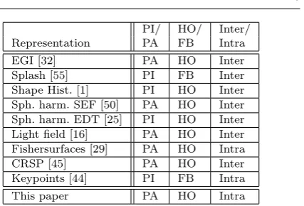
The 3D object retrieval literature can be considered in the context of a broad three-dimensional categori-sation, namely: (i) shape representations that are ei-ther pose-invariant or pose-aligned, this relates way in which the retrieval system deals with arbitrary trans-lations and rotations of the object when representing shape; (ii) shape representations that are either holistic or feature-based, this relates to the global/local nature of the shape representation; (iii) retrieval applications that are either inter-class or intra-class [56], this relates to whether the system retrieves fundamentally different object classes (car, table, vase) or different instances of the same class, as in 3D face recognition applica-tions. Of course, this is not the only categorisation and not all 3D retrieval systems fall neatly into these cate-gories, but this is a useful initial framework to discuss the literature. An example of how a small, but broad cross-section of recent work falls into these categories is given in table 1, and we use these three categories to develop our literature discussion in the following three subsections.

2.1.1 Pose-invariant and pose-aligned descriptors

Typically, pose-invariant, holistic descriptors are posi-tioned at the centre of mass of the object and are based on spherical representations encompassing the whole

PI/ HO/ Inter/

Representation PA FB Intra

EGI [32] PA HO Inter

Splash [55] PI FB Inter

Shape Hist. [1] PI HO Inter

Sph. harm. SEF [50] PA HO Inter

Sph. harm. EDT [25] PI HO Inter

Light field [16] PA HO Inter

Fishersurfaces [29] PA HO Intra

CRSP [45] PA HO Inter

Keypoints [44] PI FB Intra

This paper PA HO Intra

Table 1 A comparison of a selection of 3D object retrieval meth-ods. First column, pose-invariant (PI) or pose-aligned (PA). Sec-ond column, holistic (HO) or feature-based (FB). Third column, inter-class or intra-class retrieval tasks.

object shape. An early example is Ankerst et al’s 3D shape histograms [1], which decompose the shape into a set of concentric shells centred on the object’s centre of mass. The object surface area intersected by each shell is stored in a histogram indexed by shell radius, thus giving a 1D array of values to represent global shape.

Often 3D shape has been described as a function on a sphere [32] [50] [25] and this provides the opportunity to compactly describe shape in the spectral domain, us-ing spherical harmonics. These are a set of orthogonal functions that originate from the angular part of the solution to Laplace’s equation, expressed in polar coor-dinates. The low order amplitude coefficients of a spher-ical harmonic shape decomposition capture gross shape, while higher order coefficients represent the higher spa-tial frequencies, such as fine surface detail. Typically, phase information of the spherical harmonic function is discarded (for pose-invariance) and thus the ampli-tude information provides a pose-invariant shape de-scription.

performance than the original PCA-aligned descriptors, depending on the class of object being retrieved.

The main advantage of pose-invariant, holistic rep-resentations is that they allow fast matching, both be-cause pose alignment is not necessary, and also bebe-cause the descriptors tend to be quick to extract and pro-vide compact representations for fast shape matching. Conversely, the main disadvantage of these represen-tations is that, when discarding pose-dependent data, some pose-independent information is lost which can lead to a reduction in the descriptors power to dis-criminate between different object classes. Indeed, when such descriptors are designed, the aim is to achieve in-variance with a minimal compromise in discriminating power.

In contrast to pose-invariant techniques, whole 3D objects may be aligned before matching them and this can be done in two ways: (i) by exhaustive search for an optimal alignment between each pair of objects (probe and gallery), which is typical in inter-class retrieval problems or (ii) by aligning to some common canonical view of the stored models, which is the case of pose-normalisation, and is typical in intra-class retrieval prob-lems.

An example of exhaustive search is the light field de-scriptor approach [16]. Here silhouette images are gen-erated from projections down to 2D images over the full view sphere. These 2D images are characterised by Zernike moments and Fourier coefficients and matched over all possible alignments. Although this approach is computationally expensive, it generates highly descrip-tive shape representations that have performed well in inter-class retrieval tasks [54].

The simplest and most efficient way to align to a canonical view is to use the three principal axes of the object surface data, computed using some variant of principal component analysis (PCA). Ankerst et al [1] used this approach when augmenting their shell-based shape decomposition with sectors. However, in its raw form, this can be unreliable when comparing objects of the same class [25], for example, in arbitrary pose 3D face recognition when some of the shoulder area is included in the scan. Further problems that many PCA based approaches need to solve are: a 180 degree ambiguity in the direction of the principal axes, prin-cipal axes may switch for shapes that have eigenvalues similar in value, and a vulnerability to outliers in the raw shape data. Recently, Papadakis et al [45] have ad-dressed the pose normalisation problem in inter-class retrieval by applying PCA on both surface points and surface normals (separately). For each query/dataset comparison, both alignments are compared and the dis-tance metric with the smallest value is selected as the

match score. The representation that they develop is called a concrete radialized spherical projection (CRSP, detailed in table 1) and this has given excellent retrieval performance on the Princeton Shape Benchmark.

An alternative to PCA based alignment is to align directly to an object template already in canonical pose. Given a set of point-to-point correspondences on a pair of 3D objects that we wish to align, several research groups have shown that we can compute the relative ro-tation between the two sets of data using least-squares techniques [23], [2], [28]. Once we have the 3D rota-tion, the relative 3D translation can be computed using the means of the two data sets. The question then be-comes: how do we determine point-to-point correspon-dences? In theiterative closest points (ICP) approach of Besl and McKay [6], point-to-point correspondences are determined by using the minimum Euclidean dis-tance (closest points) across the two 3D data sets and these correspondences are iteratively refined, as align-ing rotations and translations are computed for each set of new correspondences, until the alignment algorithm converges. If ICP converges successfully, this generally occurs in a relatively small number of iterations, but the algorithm has the disadvantage of converging to local minima if the initial misalignment is too great. To avoid this, an initial estimate of the transformation between the two surfaces is generally achieved with a coarse correspondence scheme, such as that used by Lu [42], where heuristics applied to local, curvature based shape indices are used before application of ICP. Chetverikov et al [17] have developed a ‘trimmed’ version of ICP in order to improve robustness. Alignment can also be achieved by localising three or more landmarks on the 3D surface and transforming these into the canonical frame [12]. Often this is used as a coarse initial align-ment method and ICP is used as a refinealign-ment.

The main advantage of pose-aligned (view-based) descriptors is that they can be highly discriminating, as no information is ‘washed out’ in order to achieve pose-invariance. The disadvantages include the high com-putational cost of exhaustive search for alignment, or the non-trivial problem of localising landmarks for pose normalisation to a canonical view.

2.1.2 Holistic and feature-based representations

[29]. The disadvantage of such representations is that they are vulnerable to occlusions and shape deforma-tions, such as may be encountered in deformable or ar-ticulated objects. Conversely, feature based approaches extract local features, typically at distinctive points on the 3D surface, such as curvature extrema. The global distribution of such local features can be used in struc-tural (graph) matching procedures to match between a probe and gallery graph [44], or the features may be used in hashing procedures [55]. The advantages of such feature-based approaches is that they have immunity to missing parts, such as occurs from self occlusion in 2.5D shape data.

2.1.3 Inter-class and intra-class applications

The category of approach adopted has been depen-dent on the form of the 3D object retrieval task. In general, pose-invariant, holistic descriptors have been applied to inter-class retrieval problems. For example, spherical harmonic approaches [37][25] have been ap-plied to the Princeton Shape Benchmark inter-class re-trieval problem [54]. This accords with the need for compact, efficient, whole-shape descriptions for search-ing large 3D datasets. (A notable exception to this is Chen et al’s light-field descriptor (LFD) method [16], which is a large, view-based representation. With this rich information representation, the LFD system re-trieval accuracy was reported to be highly competi-tive with other methods [54].) In contrast, for intra-class retrieval applications, such as the 3D face recog-nition applications [36] [31], most researchers have used pose-aligned or pose-normalised descriptors. This ac-cords with the notion that the discriminating power of aligned/normalised descriptors is required to give the necessary fine-grained classification performance [56].

2.2 Local surface descriptors for landmark localisation

The system presented in this paper uses novel 3D sur-face descriptors for landmark localisation prior to pose alignment or pose normalisation. Thus we now look at previous work related to local 3D surface descriptors used for 3D alignment in both recognition and retrieval applications, with particular emphasis on the work ap-plied to 3D facial surfaces.

Historically, many researchers have sought to ex-tract pose invariant 3D surface descriptors. For exam-ple, Besl and Jain [5] used Gaussian curvature and mean curvature to categorise surface shape into eight distinct categories. Dorai and Jain [22] developed this to de-fine two new measures, called the ‘shape index’ and ‘curvedness’. Colbry et al [20] use shape index for what

they term anchor point localisation. Chang et al [14] use mean curvature and Gaussian curvature to localise the nose tip, nose bridge and eye cavities in 3D face data.

Gordon’s work [26] on developing curvature maps for 3D face data was an early example of a local, invari-ant 3D facial surface characterisation. This curvature was generated with a view to generating discriminat-ing features for recognition rather than localisdiscriminat-ing facial landmarks. However, extrema of curvature have since been used to generate regions of interest over which more discriminating and computationally expensive lo-cal descriptors can be extracted to determine a reliable landmark localisation [12].

Three particularly notable local 3D surface descrip-tors were presented in the 1990s; splash representations [55], point signatures [19] and spin images [35]. Stein and Medioni [55] proposed the ‘splash representation’ to encode local 3D surface shape. Here, a local con-tour is extracted, that is some fixed geodesic distance from a vertex and surface normals are generated at fixed angular displacements within the tangent plane of that vertex. The angle of the surface normals along the geodesic contour, with respect to the vertex normal, are computed and used as a mechanism for identifying a vertex. The representation is used in a hash table 3D object indexing/retrieval approach, which the authors call ‘structural indexing’.

Chua and Jarvis [19] present an alternative, which they call the ‘point signature’ representation. Here, a sphere is centered on a vertex to provide an intersect-ing curve,C, with the object surface, that is some Eu-clideandistance from the vertex. The normal of a least-squares plane fit of the points inCand the vertex itself define a reference plane and the heights of the points on the curve, C, relative to this reference plane gives a signed distance profile. Comparison of signatures is made by scanning the signed distance values out from the maximum distance value. If there are several local maxima, the comparison is executed at each local max-imum. Point signatures have been used for 3D facial feature detection and 3D face recognition [18], [60].

multi-resolution pyramids of spin images [21] in order to speed up the matching process. Other researchers have used spin images to localise 3D facial features [12].

Some approaches to 3D facial landmark localisation have adopted rules based on local surface descriptors and their distribution. For example, Xu et al [62] select nose candidate vertices as those points that have maxi-mal height in their local frame. Many of these are elimi-nated, based on the mean and variance of neighbouring points projected in the direction of the vertex’s nor-mal. Final selection of the nose position is based on the most dense collection of nose tip candidates. Segundo et al [53] developed a heuristic technique for nose tip localisation, using empirically derived rules applied to projections of depth and curvature.

An alternative approach to matching local surface descriptors in order to localise 3D surface landmarks, is to use a 3D model, marked up with the relevant landmarks, and then globally align the manually an-notated model to the data. The landmarks can then be mapped directly from the model into the data, for ex-ample, as closest vertices. This approach was applied to 3D faces by Whitmarsh et al [61]. The key step is the registration process, which uses ICP for a rigid trans-formation (translation and rotation) and a scaling step, to independently match the height width and depth of the model to that of the data. This approach appears promising, due to its efficiency in localising multiple landmarks simultaneously. However, the method relies on ICP convergence, which is difficult to guarantee in uncropped, arbitrary pose data.

2.3 RBF surface modelling

We use a radial basis function (RBF) model of the 3D facial surface in all four processing stages presented in this paper and so we now present an overview of this 3D surface modelling approach. Scattered data inter-polation using radial basis functions has been studied from at least the 1980s [24], with notable contributions by Savchenko et al [51] and Carr et al [11]. Essentially, a 3D object surface is represented implicitly (where the RBF has the value zero), which provides a compact rep-resentation with inherent interpolation abilities, since the RBF is defined everywhere inℜ3_.

Applications have been widespread and include: au-tomatic mesh repair in range-scanned graphical models [11], cranioplastic skull model repair [10], surface re-construction in ultrasound data [49], 3D shape trans-formation [58] and animated face modelling [15], where an RBF is used to transform corresponding 3D fea-ture points between a template face and a face scan.

However, the use of RBFs specifically for 3D facial fea-ture descriptors is currently sparse and the only re-lated RBF-based 3D face feature extraction that we are aware of is that of Hou and Bai [33], who use RBFs to detect ridge lines on 3D facial surfaces. This lack of literature is possibly because of the perception of RBF fitting and evaluation being computationally ex-pensive. Indeed, conventional methods for RBF implicit surface fitting to N points requires O(N3) operations and O(N2) storage, whereas our implementation em-ploys the fast multi-pole method (FMM) developed by Greengard and Rokhlin [27] and used by Carr et al [11] for interpolating 3D object surfaces. In this method, approximations are allowed in both the fitting and eval-uation of the RBF. For example, for RBF evaleval-uation at a particular point, the centres are clustered into ‘near field’ and ‘far field’. The contribution of only those cen-tres ‘near’ to the evaluation point are directly evaluated and those ‘far’ from the evaluation point are approxi-mated, allowing a globally supported RBF to evaluated quickly to some prescribed accuracy. This method re-quiresO(N logN) operations andO(N) storage for the fitting process. For evaluation of the RBF at M points, the algorithm requiresO(N logN) setup operations fol-lowed byO(M) operations.

In our work, we closely follow the approach and no-tation of Carr et al [11]. To briefly recap from their work, aradialfunction has a value at some point in n-dimensional spacex, which only depends on its 2-norm relative to another point, called a ‘centre’. Hence, in our case, the radial function value is constant over a sphere. A radial basis function uses a weighted sum of basis functions to implicitly model a surface, where the basis function may be Gaussian, cubic spline or some other function, which is radial in form, as shown in equation 1,

s(x) =p(x) +

Nc

X

i=1

λiΦ(x−xi) (1)

For our 3D facial surface RBF model,pis a linear poly-nomial,λi are the RBF coefficients,Φ is a biharmonic

spline basis function such that Φ(r) = r, and xi are

theNc RBF centres. In fitting a 3D surface, s is

cho-sen such that s(x) = 0 forms a surface that smoothly interpolates the data points xi. Thus the RBF model

parameters implicitly define the surface as the set of points where the RBF is zero. This is called the zero isosurface of the RBF. Note that one can not simply solve the equation s(xi) = 0 for our N data points, as

00 11 0 1 00 11 00 00 11 11 00 11 0011

00 00 11 11 00 11 000 000 000 000 000 000 111 111 111 111 111 111 000 000 000 000 000 000 000 111 111 111 111 111 111 111 00 00 00 00 00 00 00 00 11 11 11 11 11 11 11 11 00 00 00 00 00 00 00 00 11 11 11 11 11 11 11 11 0000 0000 0000 0000 1111 1111 1111 1111 0000 0000 0000 0000 0000 1111 1111 1111 1111 1111 positive distance to surface (DTS)

negative distance to surface

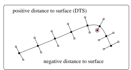
Fig. 1 Adaptive generation of ‘off surface’ points along the sur-face normal directions of a nose profile. The point marked in solid red and circled been adapted and brought nearer to the facial sur-face.

surface normal data,scan be chosen to approximate a signeddistance to surface(DTS) function.

Figure 1 illustrates the cross-section of a nose, where surface normals are used to generate off-surface points with known (signed) DTS values. In this process, care is essential at regions of high local curvature. In such cases, the distance to the surface has to be reduced on the concave side of the surface in order to avoid generating inconsistent DTS data. Our implementation employs the simple approach of Carr et al [11], which is to validate an off-surface sample point by checking that its nearest surface point is the point,p, from which it was projected. If this is not the case, then the projection distance is progressively reduced until the nearest point isp.

We use the biharmonic spline as the RBF basis func-tion, as this is known to be the smoothest interpolant in the sense that it minimises a certain energy functional associated with the fit, producing an implicit surface with minimal curvature. Thus it is well suited to repre-senting 3D object surfaces [11]. We perform a globally supported RBF fit and when we have performed the fit once, it can be evaluated anywhere inℜ3_{where we need}

to determine a signed distance to the object surface, through all four stages of the depth map generation process described in this paper. By convention, points below the facial surface (inside the head) are negative, those above the facial surface are positive and those on the facial surface are zero.

3 Spherically-sampled RBF (SSR) descriptors

In spin images [35], a surface point uses its associated surface normal to form a basis with which to encode neighbouring points. Neighbouring point positions are encoded in cylindrical coordinates, as the radius in the tangent plane and height above the tangent plane. All points are binned onto a fixed grid. Corresponding 3D

points across a pair of similar objects can be matched by a process of correlation of spin images or any other matching metric. Issues in spin image generation in-clude (i) noise affecting the computation of the local surface tangent plane and (ii) problems of appropriate bin size selection. Due to these issues, we were moti-vated to make use of an RBF model to generate invari-ant 3D surface descriptors, which we call spherically-sampled RBF(SSR) surface descriptors.

3.1 SSR shape histograms (‘balloon images’)

Here we propose a new kind of local surface representa-tion, which can be derived readily from the RBF model and we call this an SSR shape histogram. To generate such an SSR shape histogram, we first distribute a set ansample points evenly across a unit sphere, centered on the origin. To do this, we employ the octahedron sub division method, which, for K iterations, generates

n=αβK _{points. The constants are [α, β]}T _{= [8, 4]}T

and we use K = 3, which gives n = 512. The sphere is then scaled by q radii, ri, to give a set of

concen-tric spheres and their common centre is translated such that it is coincident with a facial surface point. (Note that this can be a raw vertex, but can also be anywhere between vertices, on the RBF zero isosurface).

If a sphere of radius ri is placed at some object

surface point, then the maximum distance of any point on that sphere from the object surface isri, implying

that typical maximum and minimum evaluated RBF values for a flat object surface region are +ri and −ri

respectively. Thus a reasonable normalisation of RBF values is to divide byri to give a typical range of [-1,

1] for normalised RBF distance-to-surface values. Such a normalisation allows RBF values distributed over a wide range of radii to be accumulated into the same local shape histogram.

The RBF, s, is evaluated at the N = nq sample points on the concentric spheres, and these values are normalised by dividing by the appropriate sphere ra-dius, ri. If this normalised value, sn = _ris, is binned

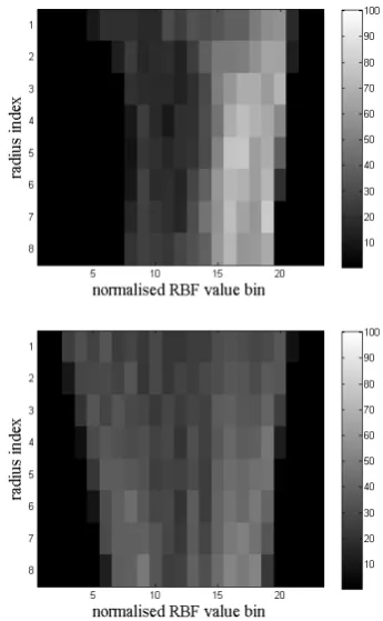
Fig. 2 Spherically sampled RBF (SSR) histograms generated over 8 radii and 23 normalised SSR bins: nose tip (upper image), forehead vertex (lower image)

3.2 SSR values

Clearly, the convexity of the local surface shape around some point is related to the brightness distribution of the balloon image. This motivates us to consider how SSR histograms may be processed to give a pose in-variant convexity value for high resolution, repeatable landmark localisation. For example, if we wish to lo-calise the nose tip, we may first define the nose tip as the point on the facial surface where a sphere of ap-propriate radius (centered on that point) and the face have minimum volumetric intersection. We then need to consider how to calculate the volumetric informa-tion from the SSR histogram and our approach is il-lustrated in figure 3. In this figure, the point p is on the object (face) surface, the upper left part of the figure is above the object surface (s(x) > 0) and the lower right part of the figure is below the object sur-face (s(x) < 0). We have illustrated three concentric spheres (solid lines) of radius (r1, r2, r3), separated by ∆r over which the RBF is sampled and we consider three co-radial samples for each of these radii atx1,x2

and x3 respectively, noting that s(x1) >0, s(x2) <0

and s(x3) > 0. The dashed circles in the figure

indi-cates the position of (non-sampling) concentric spheres

00000 00000 00000 00000 00000

11111 11111 11111 11111 11111

000000 000000 000000 000000 000000 000000

111111 111111 111111 111111 111111 111111

00000 00000 00000 00000 00000

11111 11111 11111 11111 11111

Object surface

r r

r₃ 2 1

+ +

+

x₃ x₂

x 1

p

s(x)<0 s( x )>0

Fig. 3 Computation of an SSR value, a measure of the volu-metric intersection of the object (head) and a sphere, centred on the object surface. This is an indicator of surface convexity at a selected scale. The two red shaded sectors have positive RBF evaluations and the blue shaded sector has a negative evaluation.

that bound volumetric segments, and these have radii,

ρi midway between the sampling spheres, namely at

ρi=(ri+₂ri+1). In order to determine an estimate of the

total volumetric intersection within the outer (dashed) sphere of radiusρ3=r3+∆r₂ , we need to sum all of the

volumetric contributions centred on radial sampling di-rections withs(x1)<0, over all sampling radii and all

sampling spheres.

In figure 3, the central blue shaded volumetric seg-ment contributes to the object/sphere intersection, but the two outer red shaded volumes do not. Note that the segments centred on the larger radii have bigger vol-umes, and thus a weighting vector needs to be applied to the summation. Thus the volumetric intersection,Vp,

at pointpis given by:

Vp=

k nv

T_n− ₍₂₎

where k = 4π

3 is a constant related to the volume of

a sphere, n is the total number of sample points on a sphere, vT _{is a vector containing the q volumetric}

weights (one for each radius), andn− _{is a vector where} each element is the count of the total number of sample points on a given sphere in whichs(x)<0.

An equivalent, but more elegant approach, is to de-fine a metric that is a relative measure of the volume of the sphere that is above the object surface compared with the volume of the sphere below the object surface. With this in mind, we define a SSR based convexity value for the point,p, as

Cp =

k nv

wheren+_{is a vector in which each element is the count}

of the total number of sample points on a given sphere where s(x) > 0. With this metric, a highly convex shape will have a value approaching 1.0, a highly con-cave shape will have a value approaching -1.0 and a flat area will have a value close to zero. This can be clearly seen from equation 3, where the elements inn+_andn− will be similar, giving a near zero vector on the right of the equation. In its simplest form, a very approximate SSR value can be computed using a single sphere, which makes both the constantk and the volumetric weight-ing vectorvin equation 3 redundant. We use this form in this paper, which amounts to averaging the signs of

nRBF evaluations over a sphere.

Cp=

1

n

n

X

i=1

sign(si) (4)

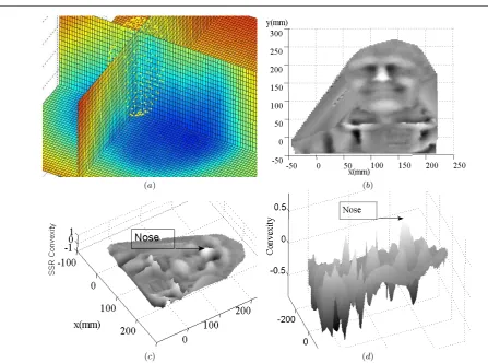
In order to illustrate the potential of this technique, a single sampling sphere of radius 20mm and 128 sample points is moved over a facial surface. Figure 4a, illus-trates the RBF distance-to-surface values of this facial surface by a colour mapping and the RBF sampling sphere (yellow) is shown positioned close to the nose bridge. The resulting SSR value map is shown from dif-ferent views in figures 4(b),(c),(d). A surface is rendered over this plot to aid visualisation, where the lighter ar-eas have a convexity value near to +1 and the darker areas are close to -1 (i.e. concave). The figure indicates that, in this case, the nose is the peak convexity value in the map. Note also that the inner eye corners have high concavity, suggesting that they are also good land-marks to localise with this descriptor.

3.3 SSR descriptors: A comparison with the literature

To our knowledge, the closest work to SSR histograms in the literature is Johnson and Hebert’s spin images [35]. Although our method requires a global set of nor-mals to computed the RBF, unlike the spin image, a local normal is not required to encode points in a lo-cal frame. We hypothesise a number of advantages that SSR histograms may have over spin images: (i) Miss-ing parts or any residual data spikes may corrupt the local normal estimate, which can have a big influence on the spin image; (ii) This is likely to be exacerbated in areas of high curvature, such as the nose tip, par-ticularly, when the raw vertex data is of limited res-olution; (iii) Missing parts can corrupt the content of spin-images, unless an effective interpolation process is implemented. For SSR histograms, the interpolation is implicit in the method, as the RBF is defined every-where in 3D space; (iv) Issue of correct bin-size selection

is an issue in spin-images, but is not a problem for SSR histograms, because we choose a set of radii explicitly; (v) Local density of points is an issue for spin images, but again this is not a problem for SSR histograms, be-cause we choose the number of sampling points on the concentric sampling spheres explicitly. In section 6, we evaluate SSR histograms and compare them to three variants of spin-image, of the same size and resolution. Given that we employ spherical methods, we now compare our approach with the general application of spherical harmonics to shape representation. Generally speaking, spherical harmonic methods have been ap-plied to global shape representations, rather than local surface representations and they have been used either to achieve pose-invariance, or to generate a compact shape descriptor for efficient matching or both. The reasons why we did not apply the Spherical Fourier Transform to our RBF ‘distance-to-surface’ function, defined on local concentric spheres are: (i) local shape descriptors need to be computed at potentially many surface points on the same 3D object, which can be computationally expensive; (ii) the SSR histogram is already inherently pose invariant for a sufficiently large number of samples on the sampling spheres and (iii) we achieve compactness by projecting the SSR shape his-togram into a reduced dimension space, using standard PCA. Nevertheless, we believe that there are several interesting avenues of research to be explored, by ap-plying spherical harmonic methods to RBF shape mod-els evaluated over concentric spheres. For example, the RBF could be evaluated over a global set of concentric spheres and spherical harmonic methods could be ap-plied to encode holistic shape in an inter-class retrieval application. This is particularly attractive when the raw 3D object data has missing parts, as is the case when shape data is derived from 3D sensor systems.

(a_{) (}b₎

(c_{) (}d₎

Fig. 4 (a) Top left shows spherical sampling of the RBF. The blue areas are negative RBF values (below the facial surface), yellow/red areas are positive RBF values (above the facial surface) and the turquoise areas contain the zero RBF isosurface (facial surface). Plots (b,c,d) in grey show the SSR values (convexity) of the same face from three different views.

at the University of British Columbia. Figure 3.3 shows the results of SIFT when applied to 60x90 depth maps from the UoY dataset. Frontal poses are shown in the left column and poses looking down are shown in the right column. All SIFT feature with scale values greater than 2 are shown and nose and eye features have been manually colored in red. Since the nose tip lies on the plane of bilateral symmetry, this often causes SIFT to generate a pair of dominant orientations for the same nose tip keypoint. This is because, in the SIFT algo-rithm, dominant directions for local gradients are de-tected as peaks in the SIFT orientation histogram. In the algorithm, the highest peak is detected and any other peak that is within 80% of this highest peak is also retained, creating a pair of coincident keypoints with different orientations. Also, as head pose changes (see figure 3.3), the dominant orientation of the keypoint changes, which is dependent on head pose; worse still, the keypoint descriptor itself must, in general, change because the changes in the depth map around a fa-cial landmark over out-of-plane rotations can not be modelled as similarity transforms, which is the class of

transforms over which the SIFT algorithm is designed to be invariant. If we compare SSR descriptors to the SIFT approach, the extrema in the SSR value func-tion are our interest points (for example maxima at nose tip, minima at inner eye corners, see fig 4) and are analagous to SIFT keypoints and SSR histograms are our descriptors, analagous to SIFT’s orientation his-togram descriptor. Both our interest point generator and descriptor are based on spherical representations in 3D as opposed to being based on a depth signal defined on an orthogonal, regular grid. This property provides significantly greater immunity to out-of-plane pose variations than is afforded by SIFT operating on single viewpoint depth maps.

4 Isoradius contours

be-Fig. 5 SIFT features (scale greater than 2) in 60x90unaligned

facial depth maps (generated by sampling UoY dataset RBF models). Frontal pose (left column) and looking down (right col-umn). Nose and eye corner features are manually colored in red.

tween any pair of faces, both of which are in non-specific poses. In this case, once the optimal alignment is deter-mined, depth maps for both faces are generated ready for feature extraction and matching. Alternatively, if a particular face (such as an average face) is known to be in canonical pose (frontal), it can act as a reference face to align all other faces in a dataset to the same canon-ical pose. This is useful when we wish to build statisti-cal models of depth map variation, which requires the depth maps to be pose-normalised.

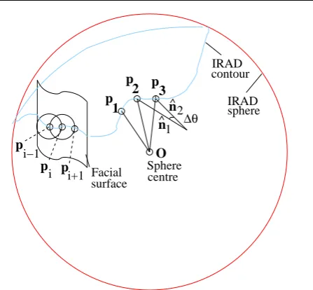
An isoradius contour is a space-curve defined by the locus on a 3D surface that is a known fixed distance relative to some predefined reference point. Thus an isoradius contour (IRAD) can be thought of as the in-tersection of a sphere, centered on that reference point, with the object surface. (We note that this is the same space-curve definition that is used in the point signature method [19], although highly sampled contours using RBF models are not used in this point signature work. In addition, we encode shape information around the contour differently, and we use the space-curve for pose alignment, rather than identification of a 3D point.)

In the case of faces, an obvious choice for the refer-ence point (sphere centre) is the tip of the nose. Clearly the shape of the intersection of the sphere with the face is independent of the 3 DOF head orientation, due to the infinite rotational symmetry of the sphere. This pose invariance is a major benefit of the representa-tion. To encode the shape of the contour, we compute its local curvature tangential to the sphere and we call this an IRAD curvature signal. If IRAD curvature sig-nals are scanned out in a consistent manner, that is in an anticlockwise direction around the nose tip normal, then these signals are pose invariant, modulo a rota-tional phase shift. This suggests that we can align a pair of faces by a process of 1D curvature signal corre-lation, applied across a pair of IRAD curvature signals

(one on each face) derived using the same sphere radius. Thus, we can generate an IRAD curvature correlation signal by sliding the smaller curvature signal exhaus-tively over the larger curvature signal. This correlation signal constrains the possible rotational alignments to a set ofn, wherenis the number of points on the larger of the two contours, typically around 150 using 1mm con-tour steps over a 30mm sphere radius. We hypothesize that the best rotational alignment occurs within this set ofnalignments, where the IRAD curvature correlation signal is a maximum.

4.1 Extracting Isoradius Contours

In order to extract an isoradius contour, we need to in-tersect a sphere of specific, known radius, with the fa-cial surface, when that sphere is centred on the localised nose tip. In order to generate an IRAD of radiusR, we make extensive use of the the RBF model that we have generated within an IRAD ‘point chaining’ procedure, which consists of the following steps:

1. Find a starting point,p1, on the facial surface.Here

‘facial surface’ is defined by the zero isosurface of RBF model. In order to do this, we generate a cir-cle, radius R, centered on the nose tip. This circle resides in a plane defined by the two eigenvectors of the point cloud around the nose tip that have the two smallest eigenvalues. This guarantees that, for a sufficiently small radius, the circle will intersect the facial surface and we simply have to interpolate any zero-crossing of the RBF (distance to surface) function evaluated on the circle, to find a starting point for the contour.

2. Localise an appropriate second point, p2 on the

fa-cial surface. We now generate a small circle of ra-diusr, centered on the starting pointp1(described

above), which sits on the surface of the IRAD sphere (shown in red in figure 6). Note that r is the step length over which we chain the IRAD contour and we user= 1mm. Again the RBF model can be used to find where this circle intersects the facial surface, by computing the RBF values over sampling points on the circle and interpolating the locations where the RBF value is zero. We obtain a pair of zero-crossings and, in contrast to step 1, here we need to choose the correct zero crossing (facial surface point), such that the isoradius contour starts to cir-cle the nose tip in a consistent, anticlockwise (right handed) sense. This is done by checking the direc-tion of the cross product between two vectors, the first of which is from the nose tip top1on the

Fig. 6 The IRAD chaining process generates a high density of points at the intersection of a sphere and the facial surface.

3. Chain IRAD points around the nose tip. Once we have foundp2, a small circle centered onp2, radius

r, and on the IRAD sphere surface can be generated. Again the RBF evaluations on this circle will have a pair of zero-crossings. This time, however, the cross product direction check is not required, because one zero crossing is very close top1and so can be ruled

out. In this way, we chain around the intersection of the IRAD sphere and the facial surface by selecting thepi+1RBF zero-crossing as the one most distant

frompi−1.

4. Terminate chaining process. When the chain comes within a threshold distance (r

2) of the start position,

then the chaining process is halted.

The IRAD chain, consisting of intersecting circles on the surface of the IRAD sphere, at the junction of the IRAD sphere and facial surface is illustrated with real data in figure 6. The ouput of this process is a set of points in 3D space that are a distance R from the nose tip and a distance r from their two neighbouring points (with the exception of the first and last point). A set of contours over a range of radii, for the purpose of illustration, are shown in figure 8. The question now is how to encode this contour and this is dealt with in the following subsection.

4.2 Encoding the contour

To encode the IRAD contour, we measure the IRAD space-curve curvature that is due to the face shape, rather than the curvature that is simply due to the fact that the IRAD is distributed across the surface of a sphere. Put simply, over a step r, the space-curve can turn to the left on the IRAD sphere surface or turn to the right, both by varying degrees, or continue straight on.

The process is illustrated at the centre of figure 7. Given that curvature,κ=∆θ∆s, and if we maintain a

con-stant step length,∆s, along the isoradius contour, then the angular changes, ∆θ, encode the contour shape.

sphere IRAD IRAD

1 ∆θ

2

i−1

Facial surface

Sphere centre

i i+1

contour

p _p

3 p

1 2

O

p p

p

n n

Fig. 7 Extraction of an IRAD and encoding of its tangential curvature

How do we actually compute ∆θ along the contour? Consider three consecutive points (p1,p2,p3) on the

contour, separated by a fixed, but small∆s, as shown in figure 7. A normal to the contour, nˆ1, is

approxi-mated as the cross product of the two vectorsOp1and

Op2, whereO is the centre of the IRAD sphere. This

vector can be recomputed for points p2 and p3 using

the cross product of Op2 and Op3 to give the vector

ˆ

n2. The change in angle of these normal vectors,∆θ, is

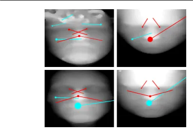
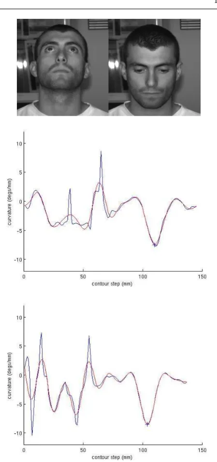
the angle that we use to encode shape in a pose invari-ant way. Given that, for sufficiently smallr, we approxi-mately move along the IRAD space-curve in even steps, this change of angle approximates a curvature, which is in a plane tangential to the IRAD sphere at the given point on the space-curve. Examples of 30mm IRAD cur-vature signals for different head poses is shown in figure 9. Note that these are approximately the same shape and differ by small phase shifts. The phase shifts are less than one might expect due to the adaptive way of generating the starting point of the contour. The fig-ure also shows how the use of a 10th order low-pass Butterworth filter can reduce noise in these curvature signals.

4.3 The effect of facial expression on IRADs

Fig. 8 Isoradius contours extracted over eleven different radii for illustration purposes. For 3D face alignment, we use a single 30mm isoradius contour, which traverses the central nose bridge area and upper lip area.

mouth open and mouth closed. The extracted contours are shown in figure 10, where the color red is used to mark ‘mouth closed’ isoradius contours and blue is used to mark ‘mouth open’ isoradius contours.

We have noted that the isoradius contours vary very little across the nose bridge and upper part of the face, whereas they do vary in the lower half of the face, the degree being dependent whether the contour falls on an area of significant surface deformation.

We are able to significantly reduce the influence of facial expression on our facial alignment process in the case when we match to a reference face in a known canonical pose. Here, we match the full isoradius con-tour of a face to be aligned (in this case, the ‘mouth open’ face), to a smaller isoradius contour that only contains the rigid nose bridge area of the reference face (in this case, the ‘mouth closed’ face). This nose bridge region provides a very strong feature for the isoradius curvature correlation to lock onto. When seeking the maximum correlation, we exhaustively shift the smaller reference contour curvature signal relative to the larger, full contour signal of the face to be aligned.

Figure 10 c, shows the isoradius contours after this alignment process (the full contours of the reference are shown in red for comparative purposes). Clearly, the upper parts of the contours are closely matched over the nose bridge area, whereas the contours in the lower part of the face are quite different. The largest two ‘open mouth’ contours marked in blue fall down into the mouth region, giving a radically different shape to the contours in the lower part of the face. Since only the upper part of the face is used in alignment, the process is successful and the result is shown in figure 10 d. Examination of this figure shows that the alignment is clearly better in the upper part of the face than the lower part. Finally, we note that the smallest IRAD

Fig. 9 IRAD curvature signals for the different head poses shown at the top of the figure. Raw curvature data is shown in blue and low-pass filtered data is shown in red. The upper graph shows the signal associated with ‘looking up’ pose and the lower graph shows signal associated with ‘looking down’ pose. The blue cross shows the manually marked position of the nose bridge in each case.

a₎

b₎

c₎

d₎

Fig. 10 The influence of mouth closed(red)/open(blue) on isora-dius contours (radii=30,38,46,54mm). a) Mouth closed. b) Mouth open. Note that isoradius contours fall under the texture map in the mouth area. c) Isoradius contours after alignment: front view and profile view (associated with d, right). d) Aligned point clouds

4.4 IRADs: A comparison with the literature

The closest related works to our concept of isoradius curvature signals are Stein and Medioni’s splash repre-sentations [55] and Chua and Jarvis’ point signatures [19]. Firstly, the splash representation generates geodesic contours around the surface, which are more difficult contours to compute than isoradius contours. Secondly, we do not attempt to extract a set of piecewise linear structural features from the data around the contour. Breaking a softly curved organic structure such as a hu-man face into a piecewise linear segments can be unsta-ble. In contrast, we extract signals that can be matched by a straightforward process of one-dimensional signal correlation. Note that, unlike ‘point signatures’ [19], we have not used a local plane normal estimate to encode our signal, as this plane (defined as the least squares fit of the contour) will be affected both by facial expression changes and missing parts. Any deviations in this plane have a global impact on the descriptor, as is the case with spin images. In contrast, our method maintains a

consistent signal for all rigid sections of the surface, re-gardless of any structural changes in other regions. For example, the curvature signal associated with the part of the contour passing through the rigid nose bridge is not affected by the same contour passing through the malleable mouth area. The tradeoff made is that the difference operators that we use to compute curvature tend to amplify surface noise, which is detrimental to performance if the facial surface defined by the RBF model is not smooth. However, we mitigate this effect with the use of a 10th order low-pass Butterworth filter applied to the curvature signals before they are corre-lated.

5 Algorithm for depth map generation

We now describe each of the four stages of generat-ing pose-normalised depth maps from noisy 3D point-clouds using our RBF model. These steps are (1) filter the data automatically (section 5.1), (2) localise the nose tip (section 5.2), (3) compute the face orientation (section 5.3) and (4) generate a pose-normalised depth map (section 5.4). Section 5.5 gives typical computation times for our system.

5.1 Automatic noise filtering

All non-synthetic 3D point cloud data, collected from 3D imaging systems, is noisy in the sense that it con-tains both spurious data, such as spikes and pits (in-ward pointing spikes), which are not associated with the surface of interest, and missing parts where no sur-face data is available. Spikes and pits generally occur due to incorrect correspondences in a stereo matching process or due to clutter in the scene. Missing parts can occur when the surface reflectance is undesirable, such as the specular surfaces on spectacles and oily skin patches, or the poor reflectance of eyebrows, facial hair and head hair. They also occur due to self-occlusion, for example, when the nose occludes the cheek in a partial side-view of the face. Many researchers have dealt with noise using very simple filtering masks on ordered data. We have designed a more sophisticated approach that does not require data ordered on a grid and establishes a self-consistent set of surface normals.

surface interpolation and our new invariant 3D feature descriptors are based. Our method of filtering the data is premised on (i) the nose being the most locally convex point that we are interested in and (ii) the inner eye corners being the most locally concave point that we are interested in within our depth map outputs. The method consists of the following steps.

1. Remove long arcs and isolated meshes. The UoY dataset contains mesh data, in addition to 3D point-cloud data and texture mapping data. We use this to remove long arcs of above 12mm and then we identify how many submeshes we have. Each of these is checked for vertex count and those below 10% of the total vertex count are removed.

2. Compute normals and DLP values.The surface nor-mal around a spherical neighbourhood (radius = 10mm) is computed by finding the eigenvectors of this localised point cloud,xi, computed using

sin-gular value decomposition (SVD). The eigenvector with the smallest eigenvalue describes the surface normal,n. We check the z-component of the normal to ensure that it is pointing away from the centre of the head towards the camera. The distance to local plane (DLP) di = n.(xi−x) is also computed as¯

a computationally cheap means of measuring local convexity/concavity.

3. Remove noisy and isolated vertices. The DLP value is compared to the mean DLP value for a set of nose vertices from 100 training images. If the vertex DLP value is greater than four standard deviations above the mean value for a nose, then the vertex is flagged as a spike. Similarly, if the DLP value is less than four standard deviations below the mean value for an inner eye corner, then the point is flagged as a pit (negative spike). If there are insufficient neighbours (less than 3) to compute a DLP value, then the point is flagged as ‘isolated’. All such vertices (spikes, pits and isolated points) are removed from the data. 4. Repeat steps 2 and 3 until there are no corrupted

normals. If there are any spikes, pits or isolated points in the neighbourhood of some vertex, then the normal of that vertex is considered corrupted. Thus both normal and DLP value for that vertex are recomputed after the corrupting points have been removed. Clearly this could generate new spikes and pits when the normal vectors adjust their orienta-tion, and so iteration of steps 2 and 3 is required un-til all normals are considered to be free from noisy data. Note that there is no data-replacement policy at this stage, which could cause some vertices to be repeatedly culled an then re-introduced.

5. Generate RBF model from valid point-set. Given a filtered set of data points, with a set of normals that

are self-consistent, it is now appropriate to generate an RBF model of the face.

6. Compute distance to surface values for noisy ver-tices and reinstate some verver-tices. We have a list of points that have been filtered from the original dataset. It is straightforward to compute the RBF ‘distance to surface’ values for this list of points with a single function call. Those vertices with a distance to surface value of close to zero can be reintroduced into the valid vertex list. This re-instatement can occur when, for example, an isolated vertex lies on the facial surface.

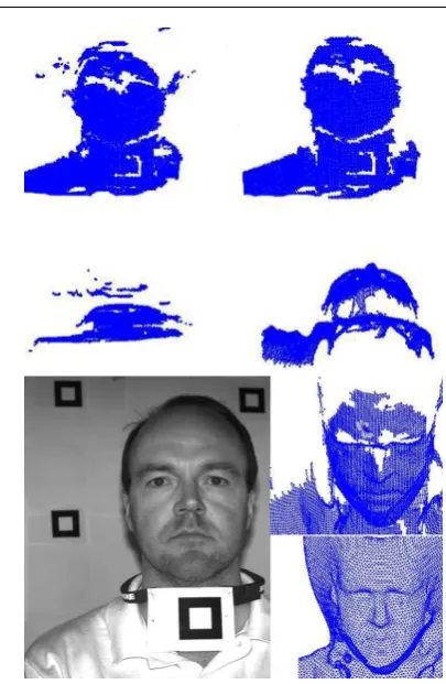
The left column of figure 11 shows typical raw data in the UoY 3D face dataset. This 3D data is shown from two views: a frontal view and a view from under the chin to show depth variations in the data. The cor-responding 2D image for which the 3D scan was taken is shown on the bottom left of the figure. The output of our filtering process for this data is shown in the right column of figure 11. The spurious data has been cleaned away successfully, but there are large gaps in the data around the brow area, for example, where we can see specular reflection in the texture image. Also in figure 11, we show a new facial mesh that has been de-rived from the zero-isosurface of the RBF, fitted to the filtered raw data. Note that this zero-isosurface mesh, generated from a standard ‘marching cubes’ algorithm [39], is used here simply to illustrate the interpolation power of RBF model fitting. Note that, in the algo-rithm described in this paper, we never need to gen-erate a global zero-isosurface, other than for the final regular grid depth map interpolation (stage 4). How-ever, a small, localised, high density zero-isosurface is generated around the identified raw nose tip vertex (in stage 3), in order to localise the nose tip to sub-vertex resolution. This is particularly useful if the nose tip area itself has missing data, either in the raw scan or due to vertex removal in the noise filtering process.

5.2 Nose tip identification and localisation

Fig. 11 The filtering process. Left column shows raw UoY data (top and middle left are 3D, bottom left is 2D ). Right column shows filtered 3D data and an RBF interpolated face (bottom-right), generated from a ‘marching cubes’ style algorithm. This is for illustration purposes: we do not need to compute this inter-polated surface in order to generate our SSR descriptors, which are highly immune to missing parts in the raw data.

by examining trained nose feature value distributions, so that the nose tip itself is never eliminated. Concep-tually, this amounts to considering every vertex as a candidate nose position, where all but one vertex are ‘false positives’. Then, at each stage, we apply a filter to reduce the number of false positives, until we have a small number of candidates at the final stage, at which point our most expensive and discriminating test is used to find the correct vertex.

The feature that we use in filter 1 is adistance to lo-cal plane(DLP), which has already been used to remove data spikes. The filter uses a weak threshold, which is four standard deviations around the average DLP value for nose tips in the training set.

In filter 2, we compute SSR values using a single sphere of radius 20mm with 128 sample points and, again, we set a weak threshold based on the Mahalnobis distance to the mean SSR value in the training data. At this stage, we have multiple local maxima in SSR value (see figure 4d) and so we find these and eliminate all vertices that are not local maxima. Finally, we use

SSR shape histograms to select the correct nose vertex by finding the minimum Mahalanobis distance to the average nose-tip in a reduced dimensional space defined by the training dataset. This nose position is refined to sub-vertex resolution by selecting the maximum SSR value over a small, local, high density zero isosurface of the RBF.

Figure 13 shows the nose candidates for each stage in the filtering process. 3D vertices are mapped into the registered texture image for clearer visualisation.

5.3 Pose computation

In section 4 we defined an isoradius contour (IRAD) and showed how to extract an IRAD curvature signal. Since head pose changes shift this signal in a rotational sense, we use a process of 1D correlation to align IRAD signals, by searching for the maximum correlation value over all possible rotational phases shifts. Of course, in the correlation process, we need to deal with IRAD sig-nals of different sizes. For now, lets suppose that the two signals are the same size. We express these signals as discrete data sets:x= [x1...xn]T andy= [y1...yn]T.

The normalised cross correlationCis given as:

C= x

T_y

p

xT_x+yT_y, where x T

x+yTy> t2 (5)

for some thresholdt. For n-1 rotational shifts of the x vector, we obtain n values of C, which yields a nor-malised cross correlation signal overnvalues.

The maximum value of the correlation signal sug-gests the correct alignment of the IRAD contour pair and we can generate a list of 3D correspondences along the matched pair of IRAD contours, as:

xq(i)→xd(j) , i= 1...n, j =i+k, modulo(n) (6)

wherexq= (x, y, z)Tq is a 3D point on the query surface,

xd = (x, y, z)Td is a 3D point on the dataset surface,n

is the number of points on the IRAD signal pair, and

k is the rotational shift (in contour steps) required to achieve the peak in correlation.

We compute these rotations using least squares [2][28]. First compute the cross covariance matrix,Kgiven by:

K=Σin=1(xq(i)−xq)(xd(j)−xd)T (7)

we then compute the singular value decomposition of Kas

K=USV′ ₍₈₎

where Sis the diagonal matrix of singular values and VandUare orthogonal matrices. The rotation matrix, R, is then given by

Junk Junk

All vertices

Junk

Refine nose tip position Junk

Filter 4 Filter 3

Filter 2 Filter 1

min

non−min local plane

Distance to

SSR value locally maximum

non−max

Nose tip vertex

input

Filter

Refine

SSR value

Interpolated nose position output

< Mahalanobis threshold

< Mahalanobis threshold

SSR histogram Mahalanobis distance

Fig. 12 The cascade filter for nose tip identification (left to right). Also shown is the sub-vertex refinement process (top right to bottom right).

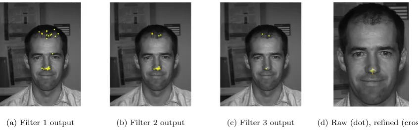
(a) Filter 1 output (b) Filter 2 output (c) Filter 3 output (d) Raw (dot), refined (cross)

Fig. 13 Vertex outputs of the cascade filter and refineprocess for nose tip identification and localisation. 3D vertices have been mapped into the associated registered 2D image for the purpose of visualisation.

In this procedure, the two signals are generally not exactly of the same length and the shorter signal is shifted and correlated across the full length of the longer signal.

5.3.1 Pose checking and refinement

When we are doing one-to-one alignments of 3D face pairs with neutral expressions, we use a pair of com-plete isoradius contours that fully encircle the nose and we find that the rotation matrix computed in 9 gives good results, which are given in sections 7.1 and 7.2. However, when we use the method to normalise to a canonical pose over large datasets containing facial ex-pressions (see section 7.3). we only use the nose bridge area of an averaged isoradius contour (using 100 3D scans) to reduce the influence of large changes in the lower facial area, such as occurs during movements of the mouth. In this case, we find that it is necessary to do checking and refinement of the rotation matrix.

Fi-nally, we can refine the rotation matrix using the RBF model, such that it gives a minimum RMS error. This can be achieved by directly computing a point corre-spondence on the RBF zero-isosurface for each point on the average face template using the following equa-tion:

xs0=xt−s(xt)

∇s(xt)

||∇s(xt)||

(10)

where xt is a 3D face template point, xs0 is its

cor-responding point on the RBF zero isosurface, where

s(x) = 0. The set of point correspondences yields a rotation matrix, as previously described, to rotate the average face template and the process can be iterated to yield a refined rotation matrix. This process is a variant of ICP, but there is no requirement to search for cor-respondences. Rather, they can be computed directly from the RBF, even in areas where the raw face data has missing parts. We find that we only need 3-4 itera-tions before rotational adjustments fall below 1 degrees, 4-7 iterations to fall below 0.5 degrees and 7-11 itera-tions to fall below 0.1 degrees. Evaluaitera-tions of these pose checking and refinement processes are given in section 7.3.

5.4 Pose-normalised depth map generation

Generation of an RBF model has provided mechanisms to localise the nose tip and determine facial orienta-tion. It also provides a futher step, namely a flexible way of generating arbitrary resolution depth maps. The method we use is a gridded coarse-to-fine search for the RBF zero-isosurface. To extract an n×mdepth map, with 8 bit depth resolution, we execute the following procedure.

1. Generate a 3D grid of size (n×m×17), which is sufficiently large to encase all 2.5D head data. 2. Translate the grid so that the nose tip is localised

at the centre of (nxm) in the X-Y plane and on the 16th row of the Z plane. (Using the 16th row rather than the 17th gives room for a sign change in the RBF at the nose tip).

3. Rotate the 3D grid about the nose tip using the rotation matrix generated by the IRAD alignment process and any RBF based pose refinements. 4. Use the RBF model to determine (nxm) sign changes

in RBF evaluations along the z-dimension (local depth dimension) of the rotated grid.

5. Populate each sign change with another (evenly spaced) 15 RBF evaluations to execute a fine-scale search for the RBF sign change. This gives an equivalent eight-bit resolution i.e. 256 depth possible values.

5.5 Average timing of our processes

We have avoided algorithms with high computational complexity in order to allow a 3D face to be processed in reasonable time. However, our prototype system is implemented in MATLAB and we have emphasized cor-rectness rather than speed optimizations that would be used in a live application. The time to process a face is dependent on the raw data size, the complexity of the surface (for example clothing in the chest and shoul-der areas), and parameter settings, such as the size of the size of spherical neighborhoods and the density of spherical sampling in SSR descriptors. In the Univer-sity of York 3D face dataset, we typically have 5000-10000 useful vertices after the automatic filtering pro-cess, which is a similar order of magnitude to FRGC data when downsampled by a factor of 4 (in two direc-tions). To give an idea of the speed of our system, we averaged the processing times over 100 facial scans. The results are as follows: (i) Normals and DLP descriptors (10mm radius neighbourhood): 4.8s; (ii) RBF model fitting: 12.1s; (iii) SSR values 40.7s (128 spherical sam-ples); (iv) SSR value local maxima 0.0003s; (v) SSR histogram generatation (4096 spherical samples) and comparison 6.5s (vi) 30mm isoradius contour extraction (1mm step length) 32.5s (vii) depth map generation (60x90 pixels, 8 bit depth) 9.9s. This gives an average processing time of around 107s per facial scan for our basic one-to-one face alignment process. These times were obtained from a PC with the following specifica-tion: AMD Athlon 64x2 Dual core 4200+ 2.20 Ghz, 4Gb RAM, running Windows XP and MATLAB R2006a.

There are two time consuming stages in our process: computatation of SSR values and generation of isora-dius contours. The time to compute SSR values is large because there are many nose tip candidates in the DLP filter output, generated from clothing in the chest and shoulder area of the scan. Typically we have to compute around 400 SSR values, but if the face is framed well, this falls to around 100 values, reducing the processing time by 30s.

6 Evaluation of nose tip identification