Parameter estimation of models with many damped complex exponentials

P a r a m e te r E s t im a t io n o f M o d e ls

W it h M a n y D a m p e d C o m p le x E x p o n e n tia ls

Margaret Helen Kahn

April 1991

A thesis submitted to the

Australian National University

for the degree of Doctor of Philosophy

Computer Sciences Laboratory,

S ta te m e n t

The results in C hapter 2 of this thesis on th e dependence of the ORA algorithm on

th e form of the constraint were obtained in collaboration w ith D r.M .R.O sborne of

th e School of M athem atical Sciences, A ustralian N ational University, and D r.G .K .Sm yth

of the M athem atics D epartm ent, U niversity of Queensland.

Elsewhere, unless otherw ise stated , th e work described is my own.

A c k n o w le d g e m e n ts

I would like to express my g ratitu d e to my supervisor, Dr. Iain Macleod, of the

C om puter Sciences Laboratory, for his continual support and interest in my research.

I am indebted to him for his painstaking reading of the drafts of this thesis. I would

also like to th an k Prof. R ichard B rent for his constructive com m ents on the content

of my work. My thanks also go to Dr. Larry Brown of the Research School of

C hem istry for suggesting the problem and providing d a ta for analysis. As well I am

grateful to Dr. Mike Osborne for stim ulating discussions on fitting exponentials.

I would also like to acknowledge th e support of th e staff of the Supercom puter

Facility at th e ANU. W ith o u t th e provision of access to th e Fujitsu VP100 and their

cheerful advice, this thesis would have been very different.

My appreciation goes to all th e staff and my fellow students of the C om puter Sciences

L aboratory for th eir help at answering m any questions.

Finally I would like to th an k my husband, T im , and our children for th eir patience

A b s tr a c t

P aram eter estim ation techniques for d a ta m odelled as a sum of dam ped complex

exponentials are proving to be a successful alternative to Fourier transform m ethods

for spectral estim ation. This thesis investigates such techniques in the context of

NM R spectroscopy where th e models are of th e form

y(n) = 2 > /tei*ke(- i,‘ +,2’r/‘ )A‘n + e(n)

k=1

for n = 1 , . . . , N. In practice these models have m any term s and are fitted to large d a ta sets. T he resulting com putations are readily vectorized and suit a supercom ­

p u ter environm ent. W ith such com putational power, num erical problem s arising

when applying p aram eter estim ation techniques to large models can be addressed

along w ith questions about theoretical statistical properties of these alternative

m ethods.

The first technique discussed is P ro n y ’s m ethod which uses th e difference equation

satisfied by the noise free d a ta to provide an alternative reparam eterisation. This can

be shown to be statistically inconsistent and so does not lead to reliable param eter

estim ates. A statistically consistent version of P ro n y ’s m ethod, referred to as the

GRA algorithm , perform s well for small models but is shown to succum b to problems

of num erical ill-conditioning w ith increased m odel complexity.

A nother extension of P ro n y ’s m ethod, th e ORA algorithm , which was previously

th e choice of the constraint on the coefficients of the difference equation. Only

certain forms of this constraint lead to consistent param eter estim ates. Even then

th e algorithm encounters the same num erical problem s as the ORA algorithm when

applied to larger models.

An extension of P ro n y ’s m ethod being used extensively in practice is the Kum aresan-

Tufts LP m ethod. A lthough this produces good param eter estim ates at high signal

to noise its perform ance deteriorates below a threshold signal to noise level. The

dependence of this threshold behaviour on th e num erical rank of the coefficient

m atrix is explored in some depth.

As these three verions of P ro n y ’s m ethod are inadequate for NM R analysis we focus

on th e developm ent of a state space realization of th e system producing th e noise-free

signal. This leads to th e Hankel Singular Value D ecom position (HSVD) algorithm

which is shown to be equivalent theoretically to P ro n y ’s m ethod b u t displays superior

estim ation accuracy when applied to real and sim ulated data. This difference in

sensitivity to p ertu rb atio n s in th e d a ta is due to the n atu re of th e com putations in

the two approaches. The HSVD algorithm uses a singular value decom position which

is less sensitive to p ertu rb atio n s th an th e corresponding Propy step, and replaces

th e calculation of zeros of a large order polynom ial by th e solution of the eigenvalues

of a norm al m atrix.

Two-dimensional NM R experim ents provide a spectral estim ation problem th a t can

be solved by a sequence of applications of th e one-dim ensional HSVD algorithm . In

th e NM R context, no o ther technique available is reliable enough to estim ate the

param eters from th e resulting d a ta sets which are m odelled as th e sum of many

C o n te n ts

S ta te m e n t i

A c k n o w le d g e m e n ts ii

A b s tr a c t iii

1 In tr o d u c tio n 1

1.1 M otivation...

1

1.2 Fourier Transform ...

2

1.3 Non-Linear Least S q u a r e s ...

6

1.4 Autoregression and Linear P re d ic tio n ...

9

1.5 Thesis O utline... 11

2 P r o n y ’s M e th o d 14

2.1 Intro d u ctio n ... 14

2.3 Separation of Variables in the Exponential M o d e l ... 18

2.4 Gradient Condition Reweighting Algorithm ... 24

2.5 Objective Function Reweighting A lgorithm ... 29

3 E x te n s io n s and I m p le m e n t a tio n s o f P r o n y ’s M e th o d 43

3.1 In tro d u ctio n ... 43

3.2 Kumaresan-Tufts Prony M eth o d ... 48

3.3 Failure of the Truncated SVD... 51

3.4 Perturbation Analysis ... 56

3.5 Experimental R e s u lts ...63

4 A S ta te S p a ce M e t h o d for E s tim a tin g F r e q u e n c ie s an d D a m p in g s 78

4.1 In tro d u ctio n ... 78

4.2 State Space System Theory ... 79

4.3 Development of the HSVD A lgorithm ...81

4.4 Relationship to Prony’s M e th o d ... 87

4.5 Algorithm Perform ance... 89

4.6 Numerical Sensitivity of the HSVD A lg o rith m ... 107

4.7 Statistical Analysis of Frequency E stim ates... 116

5.1

Introduction

123

5.2 Two-Dimensional Spectral Estim ation...125

5.3 Estimation Procedure and E x a m p le s ... 129

6 D is c u ss io n 140

6.1

Directions for Further R e s e a rc h ...140

6.2 C o n clu sio n s...142

C h a p te r 1

I n tr o d u c tio n

1.1

M o tiv a tio n

This study on p aram eter estim ation of models of m any dam ped exponentials is m oti­

vated by th e problem of spectral estim ation in Nuclear M agnetic Resonance (NMR)

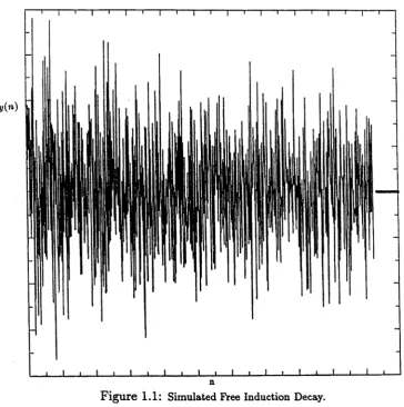
spectroscopy. The d a ta collected is th e m agnetisation of the precessing molecules in

solution as they settle to equilibrium after being p ertu rb ed by a m agnetic pulse, and

is referred to as th e Free Induction Decay (FID ). T he FID can be m odelled as a sum

of dam ped complex exponentials. For com plicated molecules th ere m ay be many

hundreds of term s in th e model. Thus the aim of this thesis is to investigate param ­

eter estim ation techniques for such models. T he features of the different algorithm s

to be discussed cover theoretical statistical foundations, com putational aspects of

th e im plem entations and possible problem s when applying these algorithm s to real

data. A m ongst other things, this will require th a t th e algorithm does not develop

num erical ill-conditioning as th e num ber of term s in th e m odel and also the num ber

of d a ta points become large.

A restriction on previous com parative studies is th e large am ount of com puter tim e

required for these analyses on conventional machines. To avoid this, it has been com­

mon practice to use estim ation m ethods which assum e statistical properties such as

statio n arity to estim ate param eters in the dam ped exponential model for which the

d a ta is not stationary. This is frequently justified on the grounds th a t the resulting

com putation tim e is minimised. However w ith the advent of supercom puters, it is

possible to concentrate on im plem enting theoretically sound m ethods rath er than

m ethods th a t m inim ise com putational tim e. Ideally, a param eter estim ation tech­

nique which gives th e best possible estim ates for noisy d a ta will satisfy statistical

requirem ents such as consistency and m inim um variance. In fact, as th e NM R d ata

is expensive and tim e-consum ing to collect, long com putation tim es for the analy­

ses are acceptable, provided the techniques used ex tract the m axim um am ount of

inform ation from th e experim ental data.

1.2

F o u rier T ra n sfo rm

T he d a ta in th e FID is collected as complex d a ta as th e m agnetisation is m easured

in two perpendicular directions. T he FID is m odelled as follows, K

y(n) =

^2

Jfc=i

for n = 1 where e(n) is complex norm al noise. The param eters and f a

represent th e am plitude and phase of th e K exponentials while 6jt and fk are the dam ping and frequency param eters and At is th e tim e interval between observations.

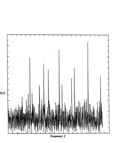
T he chem ist prefers to ex tract inform ation from th e Fourier transform spectrum of

th e noise-free tim e dom ain data. T h a t is,

V frfcA* + i2ir(fk - f ) A t

h \ rke

(6* A0 2 + (2*(/jfc - / ) At)2 ‘

This represents a sum of K complex Lorentzian lineshapes. As / —> for each k

n

Figure

damping parameters 6*. The larger

0 we approach

the line spectrum of a non-damped sum of sinusoids.

Thus the parameters of the model (1.1) can be interpreted as follows, the fk

are the

frequencies at which the spectrum has peaks, the 6* are related to the width of the

peaks and the complex amplitudes are equal to the amplitudes and phases of the

spectral peaks. Figure

shows a simulated FID and Figure

is its Fourier

transform spectrum.

There are, however, some problems with using the discrete Fourier transform on

NMR data sets. A major problem arises if the data set is truncated so that it

does not completely cover the decay of the damping parameters. This leads to

S( f )

Frequency /

F ig u r e 1.2: Fourier Transform Spectrum

leakage of peaks into the sidelobes of the transform . Possible filtering m ethods to

reduce this effect are discussed in Stephenson (1988). The m ost common m ethod

in practice is to m ultiply th e decaying FID by a bell-shaped window function. This

unfortunately leads to a loss of resolution in th e spectrum because it broadens the

peaks. Intuitively this is to be expected because there will be a loss of inform ation

from th e initial p art of the FID and this is the portion of the decaying signal with

th e highest signal to noise ratio. The artifacts introduced into th e spectrum by

th e Fourier transform and th e loss of resolution due to a tte m p ts to elim inate these

artifacts m ean th a t, for a noisy d a ta set w ith close peaks, it m ay be impossible to

separate spectral peaks or to discern signal from noise peaks.

It is because of these disadvantages of using th e Fourier transform spectrum th a t

altern ativ e param eter estim ation techniques are being developed. T he aim of such

techniques is to produce accurate estim ates of all 4K param eters in the model (1.1)

and, if so desired, these estim ates can be used to generate an estim ate of the spec­

trum .

Most results of estim ation procedures are presented as a spectral plot in this th e­

sis as it leads to direct visual com parison w ith the Fourier transform . There are

several forms of sp ectra from which to choose. T he NM R chem ist prefers to use

phase-sensitive spectra which are obtained from various quadrants of th e real and

im aginary p arts of th e spectrum . T he exam ples in this thesis are all p lotted as abso­

lute value spectra. Such sp ectra display th e sam e characteristics as a phase-sensitive

spectrum and bo th are obtained from the sam e set of estim ates of the param eters

in (1.1). Because different NM R experim ents lead to different constructions of the

phase-sensitive spectra, th e absolute value spectrum is chosen for plotting as being

m ore stan d ard .

Thus when a spectrum in this thesis is p lotted from th e estim ates of the 4K param

eters of the tim e dom ain m odel the form ula used is as follows,

K rk

S { f ) = t i (6kA 0 2 + (2x(fk ~ f W ) 2

or equivalently,

K rk

S{n) = £ [ (bkA t y + ( 2 x ( f kA t - n S W / N ) ) 2

where n = 1 , . . . , N and where S W is the spectral w idth. W hen a Fourier transform

spectrum is p lotted it is also the absolute value spectrum of the calculated discrete

Fourier transform .

1.3

N o n -L in e a r L e a st S q u a res

To fit th e m odel (1.1) to th e d a ta y ( l ) , . . . , y ( N ) a non-linear least squares problem

m ust be solved. For norm al noise, th e m axim um likelihood param eter estim ates

rk,<t>k, bk and fk m inim ise the sum of squares

K N

£

y(n) - £ r t e,**e(- ,,‘ +i2' /‘ )A<n k = 1

(1.3)

This is a non-linear optim ization problem and has th e rep u tatio n of being difficult to

solve. Any optim ization procedure used requires initial estim ates of th e param eters

to begin its iterativ e m inim isation. Badly chosen initial estim ates will lead to the

m inim isation converging (if it can) to a local rath er th a n a global m inim um .

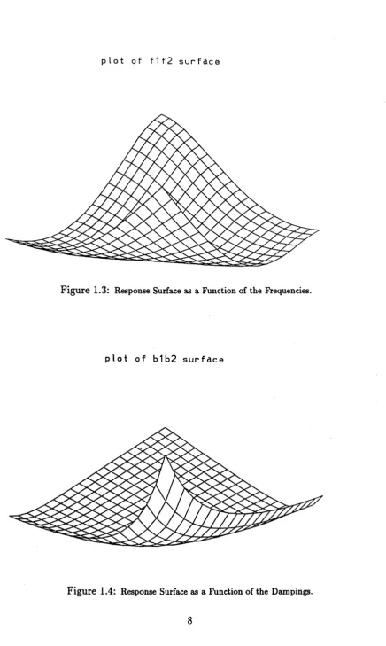
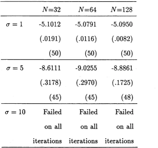
A nother difficulty w ith this least squares problem is th a t th e response surface repre­

sented by (1.3) as a function of th e 4K param eters displays large flat areas around

th e tru e p aram eter values. This m eans th a t for a large range of param eter values,

there m ay not be a significant reduction in th e sum of squares. It is not easy to find

a m inim um in such a situation.

Varah (1985) considers this problem when fitting sums of real exponentials. He

th e correct m inim um point. Sim ilar results can be shown for specific examples of

th e m odel (1.1).

Figures (1.3) and (1.4) show th e response surface at different values of the param eters

in th e m odel

yt = 2e-< cos t + 2.5e_1'5< cos l At.

By expressing the cosine term s as the sum of conjugate complex term s this model

can be w ritten in th e same form as (1.1). As there are more th an two param eters

in this case th e response surface is plotted as a function of two of th e param eters

while th e rem aining param eters are fixed at th eir tru e values. Figure (1.3) gives

a plot of the sum of squares (1.3) for varying values of th e frequencies / i and f 2.

T he tru e values of / i and / 2 are 1.0 and 1.4 and &i,62,ri and r 2 are held at their

tru e values in th e model for th e calculations. T he resulting response surface should

display a clear m inim um at th e tru e values of f i and / 2. However Figure (1.3) has a long valley shape m aking it difficult to exactly find th e m inim um . Figure (1.4)

shows th e response surface as a function of th e dam ping param eters b\ and &2 with th e frequencies and am plitudes held constant. It is even more difficult to find a

m inim um point here as the surface is m ainly flat.

Because of th e difficulty of solving this non-linear optim ization problem , alternative

p aram eter estim ation techniques are used. Most of these m ethods are known to

be sub-optim al in some way; some ignore th e decay in th e d a ta and others will

be shown to tre a t a com plicated error term as norm al noise in order to obtain a

solution. However these techniques m ay provide satisfactory initial estim ates to

sta rt th e non-linear iterative optim ization.

p l o t o f f 1 f 2 s u r f d e e

F ig u re 1.3: Response Surface as a Function of the Frequencies.

p l o t o f b 1 b 2 s u r f a c e

1 .4

A u to r e g r e s s io n a n d L in ea r P r e d ic tio n

A full review of the application of autoregressive and linear predictive m ethods to

NM R d a ta is given in Stephenson (1988) and this section sum m arises his review.

Much of th e relevant theory is drawn from Kay and M arple (1981) or can be found

in M arple (1987). The m otivation for using linear prediction comes from the com­

m only used practice of zero-filling to increase th e resolution of th e Fourier transform

spectrum . For tru n cated NM R d a ta a Fourier transform spectrum of more points

th an the tim e dom ain d a ta can be obtained by extending the d a ta set w ith zero

entries to th e required num ber of points before doing th e transform . This will pro­

duce m ore points in th e spectrum and so appear to improve the resolution but it is

not th e correct spectrum . If it is possible to predict th e shape of th e d a ta after the

tru n catio n then predicted d a ta values can be used ra th e r th an zero values. Then,

if the prediction is accurate, th e resulting Fourier transform will genuinely be of

higher resolution.

T he function used to define th e prediction relationship is the linear form

M

y ( n ) = ~ a ( m ) y ( n - m ) + e(n) (1.4)

m = l

for n = 1 , . . . , N and where e(n) is assum ed to be w hite noise. This is called Linear Prediction or LP and defines y(n) as satisfying an autoregressive (AR) model. It will be shown in C hapter 2 th a t, for d a ta m odelled as a sum of exponentials as in

(1.1), th e linear prediction relationship satisfied is actually an autoregressive moving

average (ARM A) m odel because the error term has a m ore com plicated structure

th a n ju st w hite noise.

T here are several m ethods for solving for th e coefficients a ( m) in (1.4). In sum m ary they all involve setting up a m a trix of autocorrelation coefficients which is then used

in a Levinson recursion to solve th e Yule-Walker equations to give the coefficients

a(m).

There are improvements to this method due to Burg (1967) and, as such,

the autoregressive modelling technique has been applied to NMR data, see Ni and

Scheraga (1986). There is, however, a serious problem in applying the AR modelling

to damped exponentials. The major assumption made in setting up the Yule-Walker

equations which define a recursive relationship between the autocorrelation coeffi­

cients in terms of the LP coefficients is that the data is stationary. In fact such

an assumption is crucial in defining and calculating the autocorrelation coefficients

with NMR data. This assumption is invalid because the decay in the data means

that it is not stationary. That is, statistical properties of the data such as the mean

are not constant over time. This same assumption of stationarity is required for the

Burg modification. As a result autoregressive methods are not suitable for modelling

damped exponentials. In some NMR experiments the damping is extremely light

and in this situation Ni and Scheraga (1986) and Barone et al. (1987) claim limited

success with AR modelling.

A more justifiable approach to solving for the coefficients of (1.4) is the covariance

method. In this case the LP coefficients

a(m)

are solved directly from an overde­

termined system of equations defined by (1.4). In the autoregressive modelling case

it is the normal equations arising from these equations which are used. For the

covariance method the a(m) are found as the least squares solution to the system

of equations

y = Aa,

'

y ( M +

1) N

v

y( M)

— 1)

K y ( N -

1)

y ( N

— 2)

y ( N - M )

indefi-nitely and th e Fourier transform is obtained from the z transform of the infinite d ata

set. Tang and Norris refer to this as th e LPZ spectrum . This m ethod of spectral

estim ation is not pursued any further herein for two reasons. F irstly th e LP m ethod

is purely a d a ta analysis approach and does not have any tru e statistical foundations

which are necessary for a technique to be reliable at higher noise levels. For the LP

m ethod the error e(n) is sim ply a prediction error and cannot be m odelled proba­

bilistically. The second problem w ith using th e LPZ m ethod is in the calculation

of th e spectrum . W ithout going into details, suffice it to say th a t th e calculation

involves taking th e Fourier transform of a tru n cated set of num bers. This leads to

th e sam e artifacts in th e spectrum as those seen when taking the Fourier transform

of the original data.

A m ajor disadvantage of these LP m ethods is th a t th e spectral estim ate does not

give estim ates of th e param eters in the model. Such param eter estim ates will prove

to be necessary in applications to NM R spectroscopy.

1 .5

T h e s is O u t lin e

The m ost widely used m ethod for estim ating th e param eters of th e model (1.1) is

P ro n y ’s m ethod. D etails of th e conventional P ro n y ’s m ethod are given in C hapter

2. P aram eter estim ates obtained by this m ethod are shown to be statistically sub-

optim al in th a t they are not statistically consistent. This m eans th a t, for noisy data,

increasing th e num ber of d a ta points does not necessarily im prove th e accuracy of the

p aram eter estim ates. For a statistically consistent estim ation technique increasing

the num ber of d a ta points produces param eter estim ates th a t converge to their tru e

values. In practice P ro n y ’s m ethod m ay produce adequate estim ates when the signal

to noise ratio is high bu t th e reliability of th e estim ates deteriorates rapidly as the

noise level is increased.

C h ap ter 2 also contains discussions of two modifications of P rony’s algorithm . These

are th e GRA algorithm of Osborne and Sm yth (1987) and the ORA algorithm of

Bresler and Macovski (1986). The first of these is statistically consistent while the

la tte r m ay be when a scaling constraint takes particular forms. Although both the

GRA and ORA algorithm s work well on d a ta m odelled by one or two exponentials,

neither of these m ethods proves to be robust enough to apply to NM R type models

w ith m any dam ped complex exponentials. Some reasons for this are given in the

conclusions of C hapter 2.

An extended Prony m ethod is discussed in th e work of K um aresan and Tufts (1982).

This proves to be m ore useful th an the conventional Prony m ethod on noisy d ata

sets. C hapter 3 of this thesis is devoted to a discussion of th e K um aresan-Tufts

algorithm . Spectral estim ates arising from its application to a variety of sim ulated

d a ta sets are given. This m ethod still does not produce accurate p aram eter estim ates

at m ore th an m inim al noise levels and so is not considered satisfactory for use on

experim ental data. The relationship between th e num erical rank of a coefficient

m atrix required in th e calculations and the success of the algorithm at different

noise levels is also investigated in some detail.

In C hapter 4 th e Hankel Singular Value D ecom position (HSVD) algorithm for pa­

ram eter estim ation of sums of complex exponentials is given. This algorithm is

based on a state-space in terp retatio n of the underlying system producing the noise-

free signal. This is shown to be theoretically equivalent to th e conventional Prony’s

m ethod b u t, in practice, it far outperform s any of th e Prony type m ethods. Some

theoretical justification for this is given as well as the spectral estim ates obtained

by applying th e HSVD algorithm to th e sam e sim ulated d a ta sets used in C hapter

3. Results of the analysis of a real NM R d a ta set are then presented to show a

practical application of th e HSVD algorithm . The problem of estim ating the num ­

the o u tp u t of the HSVD algorithm are discussed. This is an im p o rtan t part of the

application of param eter estim ation techniques to real NM R d a ta where the num ber

of exponentials,

K ,

C urrent experim ental practice in NM R studies is to extend th e one-dimensional

m odel to a two-dim ensional sum of complex dam ped exponentials resulting in a two-

dim ensional spectrum . Various approaches for estim ating such spectra are discussed

in C hapter 5 w ith th e final decision being m ade to use a sequence of applications of

th e HSVD algorithm . This procedure is im plem ented on some sim ulated d ata sets

to show its efficiency.

Some suggestions for future research are m ade in C h ap ter 6 and th e m ajor conclu­

sions of th e thesis sum m arised.

C h a p ter 2

P r o n y ’s M eth o d

2.1

I n tr o d u c tio n

P ro n y ’s m ethod has a long history of application to the modelling of experim ental

d a ta as th e sum of exponentials. T he original form ulation due to Baron de Prony

(1795) is used to fit K real exponentials to K d a ta points. T he technique has since

been extended to cover com plex exponentials and larger num bers of d a ta points. In

this form it is widely used in m any signal processing applications.

This chapter details the conventional P rony’s m ethod. However th e im plem entation

of the algorithm and a study of its perform ance are left to the next chapter. After

th e outline of P ro n y ’s m ethod there follows a discussion of some theoretical results

th a t show th a t th e conventional P ro n y ’s m ethod does not provide statistically satis­

factory estim ates. There are two alternative proposed m odifications. The G radient

C ondition Reweighting A lgorithm (GRA) is a modified P ro n y ’s m ethod th a t is sta ­

tistically consistent and th e O bjective Function Reweighting A lgorithm (ORA) is

shown, in a new result, to be statistically consistent when p articu lar constraints are

last two algorithm s for models w ith m any dam ped complex exponentials.

2.2

C o n v e n tio n a l P r o n y ’s M e th o d

P ro n y ’s m ethod for estim ating the param eters in a m odel expressed as a sum of

complex exponentials is a three-step procedure. Let th e d a ta be m odelled as

K

y ( n

) = ^

e^

(

.

)

k=\

for n = 1,2, . . . , 7V and where e(n) is a complex norm al random variable. For

this section we will assum e th a t th e d a ta y(n) are complex variates. For real d ata represented by a sum of K real sinusoids a m odel of the form (2.1) has 2K term s w ith each sinusoid expressed as a sum of a complex exponential and its complex

conjugate.

If the noise-free p art of th e m odel is referred to as p(n) it can be shown th a t the /x(n) satisfy a finite difference equation

K

fi(n) = — b(k)p(n — k) (2.2)

k=i

for n = K + 1 , . . . , TV. T he coefficients 6 ( 1 ) , . . . , 6(7V) are referred to as the Prony coefficients.

Now let Zk = e x p ( —bk + i 2i rf k)At and define th e polynom ial B [ z) = n £ = i(z — Zk).

Kay and M arple (1981) give a derivation of th e result th a t

B ( z ) = z K + 6(1)zk - 1 + b(2)zK~2 + •. • + b(K) (2.3)

which m eans th a t th e Zk are th e roots of th e K degree polynom ial form ed from the Prony coefficients. The frequencies and dam pings f k and bk can be obtained from th e roots Zk.

Using th e estim ates for fk and 6*. a second least squares problem can be solved to estim ate th e am plitudes r*. and phases <f>k.

In sum m ary then, the three steps of P rony’s m ethod are as follows,

i. E stim ate th e Prony coefficients b(k) in /i(n) = — Ylk=i b(k)ii(n — &)• ii. Use these estim ates to find th e zeros of th e polynom ial B ( z ) = z K -f

b( l ) z K~1 + b(2)zK~2 + . . . + b(K) = 0. iii. Solve for the r* and 0*.

Of course, in practice, we do not know the values of th e noise-free m odel /z(n) and

will have to use th e noisy d a ta y(n). As a result the results (2.2) and (2.3) become approxim ate and th e am ount of noise will affect th e accuracy of th e final param eter

estim ates.

Let th e noise-free p art of th e m odel be

fi(n) = y(n) - e(n),

then it follows th a t

K

y(n) - e(n) = /x(n) = ~ Y 1 K k ) (y(n ~ k ) ~ e(n ~ k) ) »

k=l

y ( n) = - 6(/:)y(n - A;) + ^ 6(^)e(n “ (2-4)

A:=l Jk=0

where 6(0) = 1. This is, in fact, an ARM A (autoregressive moving average) model.

Such models are difficult to estim ate. In th e NM R context w ith dam ped data,

th e usual m ethods which rely on assum ed statio n arity and th e calculation of au­

tocorrelation coefficients will be unsuitable and iterative optim isation m ethods are

In practice it is usual to ignore the moving average stru ctu re of the error term in

(2.4) and to assume th a t the model satisfies

K

y{n ) ~ - K k )y{n - k) + e(n) say. (2.5) k= l

T he Prony coefficients are then estim ated as the least squares solution to th e overde­

term ined system of equations

- b ( l ) y ( K ) - b ( 2 ) y ( K - l ) - . . . - b ( K ) y ( l ) =

—b ( l ) y ( N — 1) — b(2)y(N — 2) — . . . — b ( K ) y ( N — K ) = y( N) .

This is N — K equations in K unknowns.

The following section shows th a t the estim ates of th e Prony coefficients thus ob­

tained do not satisfy desirable statistical properties. C hapter 3 discusses num erical

problem s associated w ith solving for th e b(k). These estim ates of th e b(k) obtained

from th e above set of equations are then used as th e coefficients of th e polynom ial

B( z ) = z K + 6(1)**“ 1 + . . . + b{K). •

T he K roots of th e polynom ial are where Zk is equal to exp(—6* + i2irfk)At.

By taking logarithm s of th e **, th e estim ates of the dam pings and frequencies are

obtained.

Let £ \ , . . . ,£k be th e estim ates of the Zk and let c* = for k = 1 , . . . , K .

T hen using th e estim ates Zk in th e m odel (2.1) gives th e following system of linear

equations to be solved for the ck.

u Z2 •

. \

. Z K

A z \ . • z 2ZK

( \ Cl

, ( U

1

• _C2

=

»(2)

•

\ C K J v y ( N ) )

~ N

V $ *• • z k J v )

(

2

6

A discussion of the practical num erical considerations in solving this system of equa­

tions for dam ped d a ta is given in C hapter 3.

2 .3

S e p a r a tio n o f V a ria b les in th e E x p o n e n tia l

M o d e l

To investigate some statistical properties of P ro n y ’s m ethod of param eter estim ation

we need to retu rn to th e original nonlinear least squares form ulation of the param eter

estim ation problem discussed in C hapter 1. T h a t is, for d a ta m odelled as

K

y i n ) = J 2 c*z k + e(n)

it= i

for n = 1,2, . . . , i V , th e least squares estim ates of th e param eters ck and z k(k =

1 , 2 , . . . , K ) are obtained by solving th e m inim isation problem as follows: m inciZ (j>(c, z) where <£(c, z) = (y - fi)H( y - /*),

and y = ( y ( l ) , . . . , y {n ))T ,

and /x = (E ? =i ckz k, Ejt=i c \ z \ , • .. , E fL i $ zk ) T •

This is m ore succinctly expressed as

where A(z) is the N x K m atrix

A(z) =

Z\ z 2 ... . Z K

7 2

z i z 2 .. z lK

z \ z 2 . .. z k

Z ( z j , Z2, . . . , Z/( ) j

and c is th e vector of complex am plitudes,

C = ( c i , c 2,. . - , C K ) T .

Recall th a t ck = r kel<f>k and 2* = e x p ( —bk + i2irfk) A t in th e term inology of th e first

chapter.

Thus th e objective function to be m inim ised is

(f)(c, z) = (y - A(z)c)// (y - A(z)c). (2.8)

In th e m odel (2.1) the param eters c i , . . . , ck are referred to as th e linear param eters

of th e m odel while th e exponentials Zi, . . . ,z k are th e nonlinear param eters. An

altern ativ e b u t equivalent objective function can be obtained by separating the

linear and nonlinear param eters. Golub and Pereyra (1973) show th a t for any fixed

value of z th e sum of squares

< t>

(C, z) = (y - /i)"(y - n)

is m inim ised by

c(z) = (A //A ) _1A //y

where the notation A(z) to show the dependence of A on th e param eters in z has

been simplified for convenience.

S u b stitu tin g this expression for c(z) into (3.2) gives

t/)(z) = <j>(c (z ),z )

= (y - A ( A H A ) ~ l A H y ) H ( y - A ( A HA ) _1A " y)

= y" (I - A ( A HA ) _1A W)H(I - A ( A ff A ) _1A w)y

= y H( I - A ( A ffA ) -1A w)y

= y " ( I - P A)y (2.9)

where I is th e Nx Ndentity m atrix and i P A = A(A'^A) - 1 A -1' is th e projection

m atrix on to th e column space of the m atrix A.

Thus an altern ativ e to m inim ising the objective function <^>(c, z) is to minimise ip(z)

w ith respect to th e param eters in z and then to use these estim ates of z to find

th e estim ates of c. However this still involves a non-linear optim isation and the

objective function can be fu rth er modified by introducing th e Prony coefficients.

Define th e N x (N — K ) m atrix X as

b{K)* 0

b(K — 1)* b ( KY

x =

6

(

1

)*

6

(

2

)*

6

(

0

)*

6

(

1

)* ...

0

6

(

0

)* • • •

\

0

0

0

0

where 6(0) = 1 and * denotes complex conjugate.

Hi)*

HO)*,

It follows th a t from (2.2) th a t

B ut X ^ /i = X wA c and thus X ^ A = 0, th a t is, the columns of X and A span

orthogonal spaces.

R eturning to (2.9) we see th a t

j/>(z)

= y " ( I - P A)y

= y " P x y

= y HX ( X HX ) - l X Hy. (2.10)

This form of rp(z) becomes th e objective function for th e first step of P rony’s m ethod

and ip(z) is m inim ised w ith respect to th e Prony coefficients 6(0), 6 ( 1 ) ,..., 6(A)

ra th e r th a n w ith respect to th e param eters z of the original model. The final step

to estim ate th e complex am plitudes rem ains unchanged and an interm ediate step of

solving for the z from th e Prony coefficients is introduced. This is ju st the step of

finding th e roots of a polynom ial discussed previously.

This separation of th e variables and expression of th e objective function in term s

of th e Prony coefficients appears in the works of Bresler and Macovski (1986), Ku-

m aresan, Scharf and Shaw (1986), and Evans and Fischl (1973). It is also dealt

w ith fully in the work of Osborne and Sm yth (1987).

To show the dependence of 'ip(z ) on the Prony coefficients b we can further modify

equation (2.10). Introduce th e (N — K) x K m atrix Y as follows,

y( k + 1) y(k) _{y (i)}

y(k + 2) _{y{k + 1) •••} 1/(2)

y ( N) y ( N - l ) ■■■

It is easily seen th a t

X Hy = Y b .

S u b stitu tio n in (2.10) gives

il>(z) = xf>{b) = b HY H { X HX ) - 1Y b . (2.11)

The objective function ip is now m ore clearly shown to be a function of b. The statistical properties of the estim ates of the Prony coefficients and hence th e esti­

m ates of th e frequencies and dam pings in th e model (2.1) depend on the statistical

expected value of ^>(b), or equivalently ip(z), and the m ethod used to m inim ise it.

In th e conventional P rony’s m ethod outlined in the preceding section th e first step

of solving an approxim ate least squares problem to estim ate

b

imising an objective function

= b ^ Y ^ Y b (2.12)

in which the central term of (2.11), ( X ^ X ) - 1 , is set equal to the id en tity m atrix.

This follows from equation (2.5) where the error term e ( n) is tre a ted as w hite noise. Kay and M arple (1981) acknowledge this deficiency in P ro n y ’s m ethod and refer to

th e suboptim al conventional P rony’s m ethod as the extended P r o n y ’s method.

T he function

?/>(b)

coefficients

b

to assum e th a t a solution to the conventional Prony algorithm , (2.12), will provide

startin g values for this iteration. It is also w orth noting at this point th a t th e Prony

coefficients will be constrained in some way leading to a constrained optim ization

problem . T he usual constraint is to require th a t 6(0) = 1. T he constraint b ^ b = 1 is

also frequently used and others are possible. K ahn, M ackisack, Osborne and Sm yth

(1991) investigate the effect of th e scaling of

b

th e constrained optim isation. They show th a t it is far from trivial in m any cases.

A full statem e n t of the m inim isation problem is now given as follows,

minV>(b) = b HY H( X HX ) - ' Y b (2.13)

b

subject to the constraint 0 (b ) = 1.

T here are two proposed m ethods for solving this problem , th e modified Prony al­

gorithm of Osborne and Sm yth (1987) and the supposedly m axim um likelihood

m ethod proposed by Bresler and Macovski (1986). The differences between the two

m ethods depend on th e interrelationship between th e upd atin g of the estim ates of

b and th e solution of the statio n ary points of th e constrained objective function.

Osborne and Sm yth find th e gradient of th e constrained objective function, th a t is,

V(V>(b) + A(rf(b) - 1))

and set this equal to zero. This is th e necessary condition for the objective function

to be m inim ised subject to the constraint and A is a Lagrange m ultiplier. The

solution to this can be expressed as a nonlinear eigenvalue problem which is solved

for new estim ates of

b

GRA, th e G radient condition Reweighting A lgorithm and a full discussion of this

algorithm is given in th e following section.

Bresler and Macovski u p d ate th e objective function directly and tre a t ( X ^ X ) -1 as

constant for each iteration. This reduces th e problem to a quadratic m inim isation at

each iteratio n . K ahn et al. refer to this as ORA, th e O bjective function Reweighting

A lgorithm . Bresler and Macovski call it th e IQML algorithm for Iterativ e Q uadratic

M axim um Likelihood. Section 2.5 of this chapter shows, however, th a t the resulting

estim ates are not m axim um likelihood.

2 .4

G r a d ie n t C o n d itio n R e w e ig h tin g A lg o r ith m

In this section it will be assum ed th a t real models are being used, th a t is

K

y ( n) = ocke~ßktn (2.14)

k = i

for n = 1 , 2 , . . . , TV and where a k is real and ß k has a positive real p art and, if the im aginary p a rt is non-zero, then the complex conjugate of ß k also occurs with the sam e a k. This leads to models of th e form

K

y ( n ) = a k e ~ 0ktn cos ( f kt n + <t>k)

k=i

where, in this case, the ß k are real. T he real and im aginary p arts of the complex NM R Free Induction Decay can be m odelled in this way w ith K equal to twice the

num ber of peaks.

To discuss some statistical properties of the estim ates of

b

asym ptotic behaviour of th e estim ates as th e num ber of d a ta points tends to infinity.

For tran sien t d a ta if t n becomes infinite as n increases, for exam ple t n = n, then u ltim ately th e d a ta being collected gives no inform ation on the m odel param eters.

For large enough n th e d a ta would ju st be noise. We thus require th a t the num ber

of observations becomes infinite while t n rem ains w ithin a finite tim e interval. This interval is chosen to be [0,1] and, for exam ple, for equally spaced points in tim e

t n = n / N .

Osborne (1975) and O sborne and Sm yth (1987) show th a t the objective function

V>( b) = bTY T(XTX ) - 1Yb

= y TX (X TX )_1 X r y

is independent of the scaling of

b

bTb

elem ents of

b

to be a m inim um is achieved when its gradient w ith respect to b is zero, th a t is

(B (b ) - AI)b = 0.

In this form ula A is the Lagrange m ultiplier and B is the

(K

(K +

m atrix function of b w ith elem ents

B

rs - y

where X , = th a t is, a m atrix of zeros and ones.

T he fact th a t 0 ( b ) is independent of the scale of b implies th a t A = 0 and the

iterativ e optim isation proceeds as follows: Given an estim ate b

^

(B (b W ) - A(*+1)I)b<fc+1>

=

b(fc+1)Tb (fc+1) = 1

w ith A^+1) being the eigenvalue nearest to zero of B ( b ^ ) and

b^k+v>

ing eigenvector.

This can be solved by the m ethod of inverse iteratio n and details of its im plem en­

ta tio n are given in O sborne and Sm yth (1987). The sim ilarities between the GRA

m ethod and P isarenko’s m ethod for frequency estim ation of purely harm onic d ata

are outlined in K ahn et al. (1991). In Pisarenko’s m ethod th e solution for the coef­

ficients b is given by th e eigenvector corresponding to the eigenvalue closest to zero

of th e variance-covariance m atrix.

It is also shown in O sborne and S m y th ’s work th a t estim ates of th e Prony coeffi­

cients obtained by this m ethod are statistically consistent. T h a t is, as the num ber

of d a ta points becomes infinite th e estim ates of th e elem ents of b tend to the true

values which can be calculated as elem entary functions of th e dam ping param eters

of th e model. One problem w ith the conventional P ro n y ’s m ethod is th a t the lim ­

iting values of th e coefficients for the recurrence m odel discussed here are in fact

ju st m ultiples of th e binom ial coefficients and do not give any inform ation about

the dam ping param eters. Osborne and Sm yth prefer to use an alternative form for

th e initial difference equation (2.2). Their difference fo rm leads to a theoretically rigorous developm ent of th e asym ptotic statistical behaviour of estim ates of

b

tain ed by th e GRA algorithm . T he behaviour of th e recurrence fo rm can be derived from th e results for the difference form. However as the recurrence form given in

(2.2) is th e form ulation in com m on usage this thesis will not expand on the differ­

ence form ulation except to acknowledge its superior statistical properties. Further

discussion appears in K ahn et al. (1991).

At this point it is worthwhile showing th a t the conventional Prony procedure does

not lead to statistically consistent estim ates of

b.

th a t th e conventional Prony m ethod minimises

bTY TYb

</>(b)

necessary conditions for this are

Y r Yb = AV^»(b)T

where

A

W riting y(i) = fi(U) + e,- = m + et- for i = 1 , . . . , N where et- ~ N (0, cr2) and the et- are independent we have th a t, as n —► oo,

1 T

- Y t Y

(

(h k+i + ejc+i) ••• (/*n + ejv)

^

(/H + ei)

f

(

^ (/ijV + ejv) • * • { f ^ N - K + cN - k ) I

Jo

' 1 . . . ^

+ <t2I + negligible term s.

\

exponentials in the model. The second term is the lim iting contribution of the

stochastic p art of Y TY and it is th e same order of m agnitude as the contribution

from /i. This m eans th a t th e objective function used in the conventional Prony’s

m ethod has a significant portion which is subject to the random variability of the

data. T he resu ltan t Prony coefficient estim ates will also be highly variable for

significant noise. So P ro n y ’s m ethod is inconsistent, th a t is, the estim ates of b do

not converge to th e tru e values as the num ber of d a ta points increases in a finite

interval. For d a ta sets w ith high signal to noise ratio this will not be of great concern

b u t for low signal to noise it m eans th a t th e usual im plem entation of P ro n y ’s m ethod

is not a reliable estim ation technique.

R eturning to th e GRA m ethod, it is shown by Osborne (1975) and Osborne and

Sm yth (1987) to perform well on real, non-sinusoidal d a ta w ith relatively few term s

in th e model. K undu (1990) extends the GRA m ethod to complex d a ta and shows

th a t for one p articu lar m odel good estim ates of th e param eters are obtained. These

estim ates also satisfy desirable asym ptotic properties such as statistical consistency.

However the GRA m ethod does not appear to be as successful at estim ating the

param eters of models typical of NM R data. Keeping in m ind th e u ltim ate goal of

finding a successful estim ation technique for very large models it is unlikely th a t

asym ptotic conditions will prevail. Even d a ta sets of 1024 points are small when

hundreds of param eters have to be estim ated. For large models considerations of

num erical stability and sensitivity also become im p o rtan t.

T he im plem entation of th e GRA m ethod displayed extrem e sensitivity at two points

in th e algorithm . T he first was in th e calculation of (X TX ) -1 during the derivation

of th e m atrix B . A lthough X TX is theoretically positive definite, in practice this

property fails and various ad hoc m easures m ust be taken to continue the calcula­

tions.

The second problem area is that in finding the solution to (2.16), that is in finding the

eigenvector corresponding to the smallest eigenvalue, we are solving for the b which

makes B singular. So for a b which gives an eigenvalue close to zero, the matrix B is

nearly singular. As a result, several different package routines for finding eigenvalues

can fail if the straightforward approach of finding the zero eigenvalue is used. It is

preferable to use the inverse iteration technique to find the eigenvector of the zero

eigenvalue and Stewart (1973) suggests implementing a Cholesky decomposition of

the matrix B when solving the ill-conditioned system of linear equations that arises

in this method. However the sensitivity of the (XTX )-1 calculation is such that the

GRA algorithm is not reliable even if a refined inverse iteration step is included.

Although these problems do not appear when estimating the parameters of small

models they inhibit the application of the GRA method to NMR data with complex

models with many exponentials.

The current version of the GRA algorithm is implemented to analyse real data.

Appendix 2.1 gives a derivation of the method for solving for the complex parameters

of a complex model from the two series of real data formed from the real and

imaginary parts of the complex data series.

Kundu (1990) avoids this complication by showing that the objective function can

be minimised by differentiating with respect to the real and imaginary parts of the

complex Prony coefficients b. The matrix B thus obtained is of the same form as

(2.15) with all transpose operations replaced by complex conjugate transpose.

It is not known w hether this problem is so acute for large models.

2 .5

O b je c tiv e F u n c tio n R e w e ig h tin g A lg o r ith m

This algorithm , referred to as ORA, differs from th a t of the previous section in th a t

th e objective function ra th e r th an its gradient is tre a ted as a function of the kth

estim ate of the Prony param eters in order to find th e (k-\-l)th estim ate. This m ethod is referred to as th e Iterative Q uadratic M axim um Likelihood m ethod by Bresler and

Macovski (1986). It is also used by K um aresan, Scharf and Shaw (1986) and appears

first in Evans and Fischl (1973). It is shown in this section th a t the behaviour of the

estim ates from this technique is influenced by th e constraints applied to the Prony

coefficients. This will affect th e success of th e ORA at estim ating param eters from

d a ta w ith significant am ounts of noise. This com plication of the ORA algorithm is

not previously discussed in th e literature.

T he m inim isation problem (2.13) is restated for convenience:

m in 0 ( b ) =

br Y (X TX )_1Yb

b

subject to th e constraint

</>(b) = 1.

As in th e previous section th e discussion will be restricted to real d a ta and real

coefficients

b.

M(b) = X r X

th en

M (b(t))

M

b, b'*h

b<*+1>

b7’Y TM (b(lc))~1Yb.

T he necessary conditions for this m inim isation are

Y TM(b<*>)_1Yb = AV^(b)r

(2.18)

where A is a Lagrange m ultiplier. By com parison w ith equation (2.15) it can be

seen th a t the term corresponding to the derivative of

M(b)

th e necessary conditions. Using th e notation of Osborne (1975) this term can be

expressed as

V TV

/ _{Vi v2} n n \

. . . v n-k 0 . . . 0

j - 0 v i • • • v n-k- l v n-k • • • 0

^ 0 0 . . . V i V 2 . . . V N _ K J

and

v = M (b)-1Yb

v TX T

bTV T.

Consider th e statistical expectation of

bTV TVb

b.

£ ( b TV TVb) = £ ( v rX TXv)

= E(bTY TM (b )-1M (b )M (b )-1Yb)

= E (yr X TM (b )-

1

X y).

S u b stitu tin g

y = /z + e

X/z = 0

0

£ ( b TV TVb) = cr2tr(XTM (b)-1X)

= <72*r(M(b)"1X X T)

= a 2tr( I N- K)

= (N - K ) o r2

where £r(Ijv-*:) is th e trace of th e ( N — K) x ( N — K) identity m atrix . This is

equal to th e sum of th e diagonal elem ents of In-k- T he derivation of th e last two

lines uses stan d ard results on th e distribution of quadratic forms and th e trace of a

product of m atrices, for exam ple tfr(ABC) = i r ( C A B ) = tr(B C A ) . These can be found in tex ts such as Graybill (1961).

It can thus be seen th a t th e missing term in th e necessary conditions (2.18) becomes

norm al noise, m axim ising th e likelihood is equivalent to minimising the objective

function (2.13). As the ORA algorithm leaves out a non-negligible term in this

o p tim ization it is not a m axim um likelihood technique. However it is possible th a t,

for different constraints

0(b),

A

to statistically consistent estim ates of the Prony coefficients

b.

th e difference form ulation m entioned in the previous section and then derives the

result for th e recurrence form from th e constraint in term s of th e Prony coefficients

for th e difference form. It shows th a t large stochastic term s in th e expression (2.18)

can be cancelled by specific com binations of A and

0(b).

K ahn et al. (1991), shows th a t th e constraint should be expressible in term s of some

or all of th e squares of th e Prony coefficients, for exam ple,

||b||2

Some sim ulations follow later in this chapter to display this result.

We will now prove the less specific result th a t th e Lagrange m ultiplier is not zero

and thus th e form of th e constraint affects th e statistical properties of the ORA

algorithm . This contrasts w ith the statem en t of Bresler and Macovski th a t the

specific choice of th e scaling constraint does not affect th e final result. Both these

authors and K um aresan, Scharf and Shaw choose to incorporate other constraints

on th e Prony coefficients directly into th e calculation of th e m atrix M (b (fc)) at each

step of th e iterativ e procedure. These constraints ensure th a t th e resultant Prony

coefficients lead to dam ped or undam ped sinusoids as required by the model.

To show th a t A is not zero for th e ORA algorithm re tu rn to equation (2.18). The

gradient vector

V0(b)

V0

of Prony coefficients

b.

0(b) = ||b||2

V0

Thus we can say th a t

E (bTY TM (b)~1Yb) = A£(bTV0b).

For th e constraint

0(b)

1

jF(bTV0b)

1.

lines of the earlier proof of jF(bTV TVb) we have that

£'(bTY TM (b )_1Y b) = ^ ( y TX TM (b )-1Xy)

= (.

N - K ) ( j

2.

Thus the Lagrange multiplier A is equal to

( N — K ) a 2.

Returning to the GRA algorithm of the previous section, it can be shown that in this

case A is zero and the scaling constraint plays no part in the estimation procedure.

The proof is from Osborne and Smyth (1987). The GRA algorithm consists of

solving the generalized eigenvalue problem

(B(b) - AI)b = 0

where B satisfies equation (2.15). In this case the constraint 0(b) = ||b ||2 = 1 is

implicit. For other constraints the identity matrix is replaced by the matrix V0.

The objective function to be mimimised,

V>(b) = yTpxy

is independent of ||b|| and so a

must be orthogonal to b. That is,

t>T^ ^ = 2bTB (b )b = 0.

It follows that

b TB (b)b - b TAIb = 0

and so AI = b TB (b)b = 0 and thus the Lagrange multiplier A is zero.

This means that there is a significant difference in the implementation of the GRA

and ORA algorithms. In the former any constraint 0(b) = 1 can be used while, for

the latter, an inappropriate choice of scaling of b can lead to bad estimates.

To show the effect of the scaling constraint on the behaviour of the ORA algorithm

a simple model is used. It is

for n = 1 , . . . , TV where e(n) is normal noise.

The noise free part of the model satisfies the difference equation

T 6(2)/z1+i — 0

for i = 1 , 2 , . . . , iV — 1.

The rate constant ß is calculated from the root 2 of the polynomial 6(2) + b ( \ ) z = 0 as z — e~P/N.

The matrix Y =

»(

1

)

2

/(

2

) ^

y ( N - l )

and X T is the ( N — 1) x N matrix

/

6

(

)

(

)

(

)

(

)

(

)

(

)

V

0 0

0

6

(

)

(

)

6

(

+

(

(

)

(

)

(

)

(

)

(

+

(

(

)

(

)

0 6(1)6(2) 6(l )2 + 6(2)2

V

6

(

1

)

6

(

2

)

6

(

1)2

+

6

(

2

):

Two different constraints on b are investigated by means of simulated data sets

with increasing noise and number of data points. The two constraints used are *(*>) = |(K 1 ) + 6(2))2 = 1 and *(b ) = |(6 (1 )2 + 6(2)2) = 1.

In both cases the iterative procedure involves calculating the objective function (2.17) for the current estimate of b then minimising it subject to the particular