Terminating Distributed Construction of Shapes and
Patterns in a Fair Solution of Automata
∗Othon Michail
Computer Technology Institute & Press “Diophantus” (CTI) Patras, Greece
[email protected]
ABSTRACT
In this work, we consider asolution of automata similar to
Population Protocols and Network Constructors. The au-tomata, also called nodes, move passively in a well-mixed solution and can cooperate by interacting in pairs. Dur-ing every such interaction, the nodes, apart from updatDur-ing their states, may also choose to connect to each other in order to start forming some required structure. The model introduced here is a more applied version of Network Con-structors, imposinggeometrical constraints on the permissi-ble connections. Each node can connect to other nodes only via a very limited number oflocal ports, which implies that at any given time it has only abounded number of neigh-bors. Connections are always made atunit distanceand are
perpendicular to connections of neighboring ports. Though this variation can no longer form abstract networks, it is still capable of forming very practical2D or 3D shapes. We developnew techniques for determining the computational and constructive capabilities of our model. One of the main novelties, concerns our attempt to overcome the inherent in-ability of such systems to terminate. In particular, exploit-ing the assumptions that the system is well-mixed and has a unique leader, wegive terminating protocols that are cor-rect with high probability(w.h.p.). This allows us to develop terminating subroutines that can besequentially composed
to form larger modular protocols. One of our main results is aterminating protocol counting the size n of the system
w.h.p.. We then use this protocol as a subroutine in order to develop ouruniversal constructors, establishing thatit is possible for the nodes to self-organize w.h.p. into arbitrarily complex shapes and additionally always terminate.
Categories and Subject Descriptors:
C.2.4 [Computer-communication Networks]: Distributed Sys-tems; C.2.1 [Computer-communication Networks]: Network
∗Supported in part by the projectFOCUS, implemented un-der the “ARISTEIA” Action of the OP EdLL co-funded by the EU (ESF) and Greek National Resources.
Full version: http://arxiv.org/abs/1503.01913
Permission to make digital or hard copies of all or part of this work for personal or classroom use is granted without fee provided that copies are not made or distributed for profit or commercial advantage and that copies bear this notice and the full citation on the first page. Copyrights for components of this work owned by others than the author(s) must be honored. Abstracting with credit is permitted. To copy otherwise, or republish, to post on servers or to redistribute to lists, requires prior specific permission and/or a fee. Request permissions from [email protected].
PODC’15,July 21–23, 2015, Donostia-San Sebastián, Spain.
Copyright is held by the owner/author(s). Publication rights licensed to ACM. ACM 978-1-4503-3617-8/15/07 ...$15.00.
http://dx.doi.org/10.1145/2767386.2767402.
Architecture and Design—distributed networks, network com-munications, network topology; F.1.1 [Computation By Ab-stract Devices]: Models of Computation—automata, com-putability theory, unbounded-action devices; F.1.2 [Compu-tation By Abstract Devices]: Modes of Compu[Compu-tation— paral-lelism and concurrency, probabilistic computation; J.2 [Com-puter Applications]: Physical Sciences and Engineering—
Chemistry, Physics
Keywords: network construction; programmable matter; shape formation; population; distributed protocol; interact-ing automata; fairness; random schedule; self-organization
1.
INTRODUCTION
Recent research in distributed computing theory and prac-tice is taking its first timid steps on the pioneering endeavor of investigating the possiblerelationships of distributed com-puting systems to physical and biological systems. The first main motivation for this is the fact that a wide range of physical and biological systems are governed by underlying laws that are essentiallyalgorithmic. The second is that the higher-level physical or behavioral properties of such sys-tems are usually the outcome of the coexistence and con-stant interaction, which may include both cooperation and competition, ofvery large numbers of relatively simple dis-tributed entities respecting such laws. This effort, to the extent that its perspective allows, is expected to promote our understanding of the algorithmic aspects of our (dis-tributed) natural world and to develop innovative artificial systems inspired by these aspects.
DNA molecules into arbitrary nanoscale two-dimensional shapes and patterns [14]. Recently, an interesting theo-retical model was proposed, the Nubot model, for study-ing the complexity of self-assembled structures with active molecular components [17]. Finally a system, called the
Kilobot, was reported recently [15], that demonstrates pro-grammable self-assembly of complex two-dimensional shapes by a swarm consisting ofa thousand small, cheap, and sim-ple autonomous robots designed to operate in large groups and to cooperate through local interactions.
The established and ongoing research seems to have opened the road towards a vision that will further reshape society to an unprecedented degree. This vision concerns our ability to
manipulate mattervia information-theoretic and computing mechanisms and principles. It will be the jump from amor-phous information to theincorporation of information to the physical world. Information will not only be part of the phys-ical environment: it will constantly interact with the sur-rounding environment and will have the ability to reshape it. Matter will become programmable [7] which is a plau-sible future outcome of progress in high-volume nanoscale assembly that makes it feasible to inexpensively produce millimeter-scale units that integrate computing, sensing, ac-tuation, and locomotion mechanisms. This will enable the astonishing possibility of transferring the discrete dynamics from the computer memory black-box to the real world and to achieve aphysical realization of any computer-generated object. It will have profound implications for how we think about chemistry and materials. Materials will become user-programmed and smart, adapting to changing conditions in order to maintain, optimize or even create a whole new func-tionality using means that are intrinsic to the material it-self. It will even change the way we think about engineering and manufacturing. We will for the first time be capable of building smart machines that adapt to their surroundings, such as an airplane wing that adjusts its surface properties in reaction to environmental variables [18], or even further realize machines that can self-built autonomously.
1.1
Our Approach-Contribution
We imagine here a “solution” of automata (also called
nodes orprocesses throughout the paper), a setting similar to that of Population Protocols and Network Constructors. Due to its highly restricted computational nature and its very local perspective, each individual automaton can prac-tically achieve nothing on its own. However, when many of them cooperate, each contributing its meager computa-tional capabilities, impressive global outcomes become fea-sible. This is also, for example, the case in the Kilobot system, where each individual robot is a remarkably sim-ple artifact that can perform only primitive locomotion via a simple vibration mechanism. Still, when a thousand of them work together, their global dynamics and outcome re-semble the complex functions of living organisms. From our perspective, cooperation involves the capability of the nodes to communicate by interacting in pairs and to bind to each other in an algorithmically controlled way. In particular, during an interaction, the nodes can update their local states according to a small common program that is stored in their memories and may also choose to connect to each other in order to start forming some required structure. Later on, if needed, they may choose to drop their connection, e.g. for rearrangement purposes. We may think of such nodes as
the smallest possible programmable pieces of matter. For example, they could be tiny nanorobots or programmable molecules (e.g. DNA strands). Naturally, such elementary entities are not (yet) expected to be equipped with some in-ternal mobility mechanism. Still, it is reasonable to expect that they could be part of some dynamic environment, like a boiling liquid or the human circulatory system, providing an external (to the nodes) interaction mechanism. This, to-gether with the fact that the dynamics of such models have been recently shown to be equivalent to those of CRNs, mo-tivate the idea of regarding such systems as a solution of programmable entities. We model such an environment by imagining anadversary scheduleroperating in discrete steps and selecting in every step a pair of nodes to interact with each other.
Our main focus in this work, building upon the findings of [12], is to further investigate the cooperative structure formation capabilities of such systems. Our first main goal is to introduce a more realistic and more applicable version of network constructors by adjusting some of the abstract parameters of the model of [12]. In particular, we introduce some physical (or geometrical) constraints on the connec-tions that the processes are allowed to form. In the network constructors model of [12], there were no such imposed re-strictions, in the sense that, at any given step, any two pro-cesses were candidates for an interaction, independently of their relative positioning in the existing structure/network. This was very convenient for studying the capability of such systems to self-organize into abstract networks and it helped show that arbitrarily complex networks are in principle con-structible. On the other hand, this is not expected to be the actual mechanism of at least the first potential imple-mentations. First implementations will most probably be characterized by physical and geometrical constraints. To capture this in our model, we assume that each device can connect to other devices only via a very limited number of ports, usually four or six, which implies that, at any given time, a device has only a bounded number of neighbors. Moreover, we further restrict the connections to be always made at unit distance and to be perpendicular to connec-tions of neighboring ports. Though such a model can no longer form abstract networks, it may still be capable of forming very practical 2D or 3D shapes. This is also in agreement with natural systems, where the complexity and physical properties of a system are rarely the result of an unrestricted interconnection between entities.
be easily shown that deterministic termination of population protocols can fail even in determining whether there is a sin-gleain an input assignment, mainly because the nodes do not know and cannot store in their memories neither the size of the network nor some upper bound on the time it takes to meet (or to influence or to be influenced by) every other node. To overcome the storage issue, we exploit the abil-ity of nodes to self-assemble into larger structures that can then be used as distributed memories of any desired length. Moreover, we exploit the common (and natural in several cases) assumption that the system is well-mixed, meaning that, at any given time, all permissible pairs of node-ports have an equal probability to interact, in order to give termi-nating protocols that are correct with high probability. This is crucial not only because it allows to improve eventual stabi-lization to eventual termination but, most importantly, be-cause it allows to develop terminating subroutines that can be sequentially composed to form larger modular protocols. Such protocols are more efficient, more natural, and more amenable to clear proofs of correctness, compared to exist-ing protocols that are based on composexist-ing all subroutines in parallel and “sequentializing” them eventually by perpet-ual reinitializations. To the best of our knowledge, [13] is the only work that has considered this issue but with totally different and more deterministic assumptions. Several other papers [1, 2, 12] have already exploited a uniform random interaction model, but in all cases for analyzing the expected time to convergence of stabilizing protocols and not for max-imizing the correctness probability of terminating protocols, as we do here.
Our model for shape construction is strongly inspired by the Population Protocol model [1] and the Mediated Popu-lation Protocol model [10]. For introductory texts on popu-lation protocols see [3, 11]. For further literature related to the present work, consult the full paper and [12].
Section 2 formally defines the model under consideration and brings together all definitions and basic facts that are used throughout the paper. Section 3 introduces our tech-nique for counting the sizenof the system with high prob-ability. The main result of that section (i.e. Theorem 1) is of particular importance as it underlies all sequential com-position arguments that follow in the paper. In particu-lar, the protocol of Section 3.1 is used as a subroutine in our universal constructors, establishing that it is possible to construct with high probability arbitrarily complex shapes (and patterns) by terminating protocols. Theseuniversality
results are discussed in Section 4. Finally, in Section 5 we conclude and give further research directions that are opened by our work. In the full paper we also provide direct con-structors for some basic shape construction problems and study the problem of shape self-replication.
2.
THE MODEL
The system consists of a population V of n distributed
processes (finite-state machines), called nodes throughout. Every node has a bounded number of ports which it uses to interact with other nodes. In the 2-dimensional (2D) case, there are four portspy,px, p−y, andp−x, which for
nota-tional convenience are usually denotedu,r,d, andl, respec-tively (for up, right, down, and left, respectively). Neigh-boring ports are perpendicular to each other, forming local axes; that is u⊥ r, r ⊥ d, d ⊥l, and l ⊥ u. Similar as-sumptions hold for the 3D case. An important remark is
that the above coordinates are only for local purposes and do not necessarily represent the actual orientation of a node in the system. Nodes may interact in pairs, whenever a port of one nodewis at unit distance and in straight line (w.r.t. to the local axes) from a port of another nodev.
Definition 1. A 2D protocol is defined by a 4-tuple(Q,
q0, Qout, δ), whereQis a finite set of node-states,q0∈Qis
the initial node-state, Qout⊆Qis the set of output node-states, andδ: (Q×P)×(Q×P)× {0,1} →Q×Q× {0,1}
is the transition function, whereP = {u, r, d, l} is the set of ports. When required, also a special initial leader-state
L0∈Qmay be defined.
If δ((a, p1),(b, p2), c) = (a0, b0, c0), we call (a, p1),(b, p2), c→(a0, b0, c0) atransition(orrule). A transition (a, p1),(b, p2), c→(a0, b0, c0) is calledeffective ifx6=x0for at least one x∈ {a, b, c}andineffective otherwise.
LetE ={(v1, p1)(v2, p2) :v1 6=v2 ∈V andp1, p2 ∈P}
be the set of all unordered pairs of node-ports (cf. [12] for more details on unordered interactions). AconfigurationC
is a pair (CV, CE), where CV : V → Qspecifies the state of each node and CE : E → {0,1} specifies the state of every possible pair of node-ports (or edge). In particular, an edge in state 0 is calledinactive and an edge in state 1 is calledactive. The initial configuration is always the one in which all nodes are in state q0 (apart possibly from a
unique leader in stateL0) and all edges areinactive.
Exe-cution of the protocol proceeds in discrete steps. In every step, a pair of node-ports (v1, p1)(v2, p2) is selected by an
adversary scheduler and these nodes interact via the corre-sponding ports and update their states and the state of the edge joining them according to the transition functionδ.
Every configuration C defines a set of shapes G[A(C)], where A(C) =CE−1[1]; i.e. the network induced by the ac-tive edges of C. Observe that not all possible A(C) are valid given our geometrical restrictions, that connections are made at unit distance and are perpendicular whenever they correspond to consecutive ports of a node. For example, if (v1, r)(v2, l) ∈ A(C) then (v1, l)(v2, r) ∈/ A(C). In
gen-eral, A(C) isvalid if any connected component defined by it (when arranged according to the geometrical constraints) is a subnetwork of the2D grid network with unit distances. A validA(Ct−1) also restricts the possible selections of the
scheduler at stept ≥1. In particular, (v1, p1)(v2, p2)∈ E
can be selected for interaction (oris permitted) at steptiff
A(Ct−1)∪ {(v1, p1)(v2, p2)}is valid. Observe that any edge
that is active before step tis trivially permitted at step t. From now on, we call a 2D (3D) shape any connected sub-network of the 2D (3D) grid sub-network with unit distances.
Throughout the paper we restrict attention to configura-tions C in whichA(C) is valid. We write C→C0 if C0 is reachable in one step fromC (meaning via a single interac-tion that is permitted on C). We say thatC0 is
reachable
from C and write C C0, if there is a sequence of con-figurationsC =C0, C1, . . . , Ct =C0, such that Ci →Ci+1
for all i, 0 ≤ i < t. An execution is a finite or infinite sequence of configurations C0, C1, C2, . . ., where C0 is the
initial configuration andCi→Ci+1, for alli≥0. We only
consider fair executions, so we require that for every pair of configurationsC and C0 such that C→C0, if C occurs infinitely often in the execution then so does C0. In most
and uniformly at random one of the permitted interactions. The uniform random scheduler is fair with probability 1. In this work, with high probability (abbreviated w.h.p.) means with probability at least 1−1/ncfor some constantc≥1.
We define the output of a configuration C as the set of shapesGout(C) = (Vs, Es) whereVs ={u∈ V : CV(u) ∈
Qout}and Es=A(C)∩ {(v1, p1)(v2, p2) :v1 6=v2 ∈Vs and p1, p2∈P}. In words, the output shapes of a configuration
consist of those nodes that are in output states and those edges between them that are active. Throughout this work, we are interested in obtaining a single shape as the final out-put of the protocol. As already mentioned, our main focus will be on terminating protocols. In this case, we assume thatQout ⊆Qhalt ⊆Q, where, for allqhalt ∈Qhalt, every rule containingqhaltis ineffective.
Definition 2. We say that an execution of a protocol on
n processes constructs (stably constructs) a shapeG, if it terminates (stabilizes, resp.) with outputG.
Every 2D shapeGhas a unique minimum 2D rectangleRG
enclosing it.RGis a shape with its nodes labeled from{0,1}. The nodes of G are labeled 1, the nodes in V(RG)\V(G) are labeled 0, and all edges are active. It is like filling G
with additional nodes and edges to make it a rectangle. In fact,RGcan also be constructed by a protocol, givenG(see the full paper). The dimensions ofRG are defined byhG, which is the horizontal distance between a leftmost node and a rightmost node of the shape (x-dimension), and vG, which is the vertical distance between a highest and a lowest node of the shape (y-dimension). Let also max dimG := max{hG, vG} and min dimG := min{hG, vG}. Then RG
can be extended bymax dimG−min dimGextra rows or columns, depending on which of its dimensions is smaller, to yield amax dimG×max dimGsquareSGenclosingG(we mean here a{0,1}-node-labeled square, as above, in which
G can be identified). Observe, that such a square is not unique. For example, if G is a horizontal line of lengthd
(i.e. hG=dandvG= 1) then it is already equal toRGand has to be extended byd−1 rows to becomeSG. These rows can be placed inddistinct ways relative toG, but all these squares have the same sizemax dimG×max dimGdenoted by|SG|.
A 2D (3D) shape language Lis a subset of the set of all possible 2D (3D) shapes. We restrict our attention here to shape languages that contain a unique shape for each possible maximum dimension of the shape. In this case, it is equivalent, and more convenient, to translateL to a language of labeled squares. In particular, we define in this work ashape languageLby providing for everyd≥1 a single
d×dsquare with its nodes labeled from{0,1}. Such a square may also be defined by ad2-sequenceSd= (s
0, s1, . . . , sd2−1)
of bits or pixels, where sj ∈ {0,1} corresponds to the jth node as follows: We assume that the pixels are indexed in a “zig-zag” fashion, beginning from the bottom left corner of the square, moving to the right until the bottom right corner is encountered, then one step up, then to the left until the node above the bottom left corner is encountered, then one step up again, then right, and so on. The shapeGddefined bySd, calledthe shape ofSd, is the one induced by the nodes of the square that are labeled 1 and throughout this work we assume thatmax dimGd=d.
For simulation purposes, we also need to introduce appro-priate shape-constructing Turing Machines (TMs). We now
describe such a TMM: M’s goal is to construct a shape on the pixels of a √n×√n square, which are indexed in the zig-zag way described above. M takes as input an integer
i∈ {0,1, . . . , n−1}and the sizenor the dimension√n of the square (all in binary) and decides whether pixelishould belong or not to the final shape, i.e. if it should beonoroff, respectively. 1 Moreover, in accordance to our definition of
a shape, the construction of the TM, consisting of the pixels thatM accepts (ason) and the active connections between them, should beconnected(i.e. it should be a single shape).
Definition 3. We say that a shape languageL= (S1, S2, S3, . . .) is TM-computable (or TM-constructible) in space f(d), if there exists a TM M (as defined above) such that, for every d ≥ 1, when M is executed on the pixels of a
d×d square results in Sd (in particular, on input (i, d), where0≤i≤d2
−1, M gives outputSd[i]), by using space
O(f(d))in every execution.
Definition 4. We say that a protocol A constructs a shape language L with useful space g(n) ≤ n, if g(n) is the greatest function for which: (i) for all n, every execu-tion of A on n processes constructs a shape G ∈ L 2
of order at leastg(n)(provided that such a Gexists) and, ad-ditionally, (ii) for allG∈ Lthere is an execution of Aon
n processes, for somensatisfying |V(G)| ≥g(n), that con-structs G. Equivalently, we say that A constructs Lwith wasten−g(n).
We now give as an illustrating example, a stabilizing pro-tocol for the problem of constructing a spanning square. More protocols are given in the full paper. We assume, for simplicity, that √n is integer and that there is a pre-elected unique leader in stateLuand all other nodes are ini-tially in stateq0. The effective rules are (Lu, u),(q0, d),0→
(q1, Lr,1),(Lr, r),(q0, l),0→(q1, Ld,1),(Ld, d),(q0, u),0→
(q1, Ll,1),(Ll, l),(q0, r),0→(q1, Lu,1),(Lu, u),(q1, d),0→
(Ll, q1,1),(Lr, r),(q1, l),0→(Lu, q1,1),(Ld, d),(q1, u),0→
(Lr, q1,1),and (Ll, l),(q1, r),0→(Ld, q1,1).
The protocol first constructs a 2×2 square. When it is done, the leader is at the bottom-right corner and is in stateLd. In general, whenever the leader is at the left (the up, right, and down cases are symmetric) of the already constructed square it tries to move right in order to walk above the square. If it does not succeed, it is because it has not yet passed over the upper boundary, so it activates the edge to the right, takes another step up and then tries again to move right. In this way, the leader always grows the square perimetrically and clockwise.
3.
PROBABILISTIC COUNTING
In this section, we consider the problem of counting n. In particular, we assume a uniform random scheduler and we want to give protocols that always terminate but still w.h.p. countn correctly (or a satisfactory upper bound on
n). The importance of such protocols is further supported by the fact that we cannot guarantee anything much better than this. In particular, if we require a population protocol
1Note that if the TM is not provided with the square size
together with the pixel, then it can only compute uni-form/symmetric shapes that are independent ofn.
2Gis the shape of a labeled squareS
to always terminate and additionally to always be correct, then we immediately obtain an impossibility result.
In Section 3.1, we present a protocol with a unique leader that solves w.h.p. the counting problem and always termi-nates. To the best of our knowledge, this is the first pro-tocol of this sort in the relevant literature. Additionally, this protocol is crucial because all of our generic construc-tors, that are developed in Section 4, are terminating by assuming knowledge ofn (stored distributedly on a line of length logn). They obtain access to this knowledge w.h.p. by executing the counting protocol as a subroutine. Finally, knowingn w.h.p. allows to develop protocols that exploit sequential composition of (terminating) subroutines, which makes them much more natural and easy to describe than the protocols in which all subroutines are executed in paral-lel and perpetual reinitializations is the only means of guar-anteeing eventual correctness (the latter is the case e.g. in [8, 10, 12], but not in [13] which was the first extension to allow for sequential composition based on some non-probabilistic assumptions). In Section 3.2 we establish that if the nodes have unique ids (UIDs) then it is possible to solve the prob-lem without a unique leader.
3.1
Fast Probabilistic Counting With a Leader
Keep in mind that in order to simplify the discussion, a sort of population protocol is presented here. So, there are no ports, no geometry, and no activations/deactivations of connections. In every step, a uniform random scheduler se-lects equiprobably one of then(n−1)/2 possible node pairs, and the selected nodes interact and update their states ac-cording to the transition function. The only difference from the classical population protocols is that a distinguished leader node has unbounded local memory (of the order ofn). Later, in Section 4.1, we will adjust the protocol to make it work in our model (thus also dropping this unbounded local memory assumption).
Counting-Upper-Bound Protocol: There is initially a unique leader l and all other nodes are in state q0.
As-sume thatlhas twon-counters in its memory, initially both set to 0. So, the state of l is denoted as l(r0, r1), where r0 is the value of the first counter andr1 the value of the
second counter, 0 ≤ r0, r1 ≤ n. The rules of the
proto-col are (l(r0, r1), q0) → (l(r0+ 1, r1), q1), (l(r0, r1), q1) →
(l(r0, r1+ 1), q2), and (l(r0, r1),·)→(halt,·) ifr0 =r1.
Observe thatr0counts the number ofq0s in the population
whiler1 counts the number ofq1s. Initially, there aren−1 q0s and noq1s. Wheneverlinteracts with aq0,r0increases
by 1 and the q0 is converted to q1. Whenever l interacts
with aq1,r1 increases by 1 and the q1 is converted toq2.
The process terminates whenr0=r1 for the first time. We
also give tor0 an initial head start ofb, wherebcan be any
desired constant. So, initially we haver0 =b,r1 = 0 and i= #q0=n−b−1,j= #q1=b(this can be easily achieved
by the protocol). So, we have two competing processes, one countingq0s and the other countingq1s, the first one begins
with an initial head start ofband the game ends when the second catches up the first. We now prove that when this occurs the leader will almost surely have already counted at least half of the nodes.
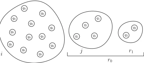
Theorem 1. The above protocol halts in every execution. Moreover, if the scheduler is a uniform random one, when this occurs, w.h.p. it holds thatr0≥n/2.
j i
q0
q0
q0
q0
q0
q1
q1
q1
q1
q0
q0
q0
q0
r1
q2
q2
r0
q0
q0
[image:5.612.319.553.53.156.2]q0
Figure 1: A configuration of the system (excluding the leader).
Proof. The random variableidenotes the number ofq0s
andjdenotes the number ofq1s in the configuration, where
initially i=n−b−1 and j=b. Observe also that all the following hold: j=r0−r1,r0≥r1,r1 = (n−1)−(i+j),
and r0+r1 is equal to the number of effective interactions
(see Figure 1).
Given that we have an effective interaction, the probabil-ity that it is an (l, q0) ispij=i/(i+j) and the probability
that it is an (l, q1) isqij= 1−pij=j/(i+j). This random
process may be viewed as a random walk (r.w.) on a line withn+ 1 positions 0,1, . . . , nwhere a particle begins from positionband there is an absorbing barrier at 0 and a reflect-ing barrier atn. The position of the particle corresponds to the differencer0−r1of the two counters which is equal toj.
Observe now that ifj≥n/2 thenr0−r1≥n/2⇒r0≥n/2,
so it suffices to consider a second absorbing barrier atn/2. The particle moves forward (i.e. to the right) with prob-ability pij and backward with probability qij. This is a “difficult” r.w. because the transition probabilities not only depend on the positionj but also on the sum i+j which decreases in time. In particular, the sum decreases when-ever an (l, q1) interaction occurs, in which case aq1 becomes q2. Observe also that, in our case, the duration of the r.w.
can be at most n−b, in the sense that if the particle has not been absorbed after n−b steps then we have success. The reason for this is thatn−beffective interactions imply that r0+r1 = n, but as r0 ≥ r1, we have r0 ≥ n/2. In
fact, r0 ≥n/2 ⇔j+r1 ≥n/2. We are interested in
up-per bounding P[failure] = P[reach 0 beforer0≥n/2 holds],
which is in turn upper bounded by the probability of reach-ing 0 before reachreach-ingn/2 and beforen−beffective interac-tions have occurred (this is true because, in the latter event, we have disregarded some winning conditions). It suffices to bound the probability of reaching 0 beforeneffective in-teractions have occurred. Thus, we have r0+r1 ≤n but r1 ≤ r0 ⇒ 2r1 ≤ r0+r1, thus 2r1 ≤ n ⇒ r1 ≤ n/2 ⇒
(n−1)−(i+j)≤n/2⇒i+j≥(n/2)−1 =n0. And if
we setn0= (n/2)
−1 we havei+j≥n0. Moreover, observe
that whenr0+r1=n+ 1 we haven+ 1 =r0+r1≤2r0⇒ r0 ≥ n/2. In summary, during the first n effective
inter-actions, it holds that i+j ≥ n0 = (n/2)
−1 and when interaction n+ 1 occurs it holds that r0 ≥n/2, that is, if
the process is still alive after timen, thenr0 has managed
to count up ton/2 and the protocol has succeeded. Now,i+j≥n0implies thatpj≥(n0−j)/n0andqj≤j/n0
to one in which the probabilities do not depend on j by restricting it to the prefix [0, b] of the line. In this part, it holds that j ≤ b which implies that p ≥ (n0
−b)/n0 and q≤b/n0. Now we setp= (n0−b)/n0andq=b/n0. Observe that this may only increase the probability of failure. Recall that initially the particle is on positionb. Imagine now an absorbing barrier at 0 and another one atb. Whenever the r.w. is onb−1 it will either return to bbefore reaching 0 or it will reach 0 (and fail) before returning tob. Due to symmetry it is equivalent to assume that the particle begins from position 1, moves forward with probability p0 = q,
backward with probabilityq0=p, and it fails atb. Thus, it
is equivalent to bound P[reachbbefore 0 (when beginning from 1)], i.e. the probability of winning in the classical ruin problem analyzed e.g. in [6] page 345. If we setx=q0/p0= p/q = (n0
−b)/b we have that: P[reachbbefore 0] = 1−
xb−x xb−1 =
x−1 xb−1 ≤
x xb−1 ≈
1 xb−1 ≈
1
nb−1. Thus, whenever the
original walk is onb−1, the probability of reaching 0 before reachingb again, is at most 1/nb−1. Now assume that we
repeat the above walkntimes, i.e. we place the particle on
b−1, play the game, then if it returns tobwe put again the particle onb−1 and play the game again, and so on. From Boole-Bonferroni inequality, we have that:
P[fail at least once]≤Pn
m=1P[fail at repetitionm]≤ Pn
m=1 1 nb−1 =
n nb−1 =
1 nb−2.
Remark 1. For the Counting-Upper-Bound protocol to terminate, it suffices for the leader to meet every other node twice. This takes twice the expected time of a meet every-body(cf. [12]), thus the expected running time of Counting-Upper-Bound isO(n2logn)
(interactions).
Remark 2. When the Counting-Upper-Bound protocol ter-minates, w.h.p. the leader knows anr0 which is betweenn/2
andn. So any subsequent routine can use directly this esti-mation and pay in an a priori waste which is at most half of the population. In practice, this estimation is expected to be much closer tonthan to n/2(in all of our experiments for up to 1000 nodes, the estimation was always close to
(9/10)nand usually higher). On the other hand, if we want to determine the exact value of n and to have no a priori
waste, then we can have the leader wait an additional large polynomial (inr0) number of steps, to ensure that the leader
has met every other node w.h.p..
In the full paper, we also give some evidence that the unique leader assumptionis probably necessary, but leave it as an interesting open question. In contrast, we show in the next section that it can be dropped if UIDs are available.
3.2
Counting Without a Leader but With UIDs
Now nodes have unique ids from a universeU. Nodes ini-tially do not know the ids of other nodes norn. The goal is again to countnw.h.p.. All nodes execute the same program and no node can initially act as unique leader, because nodes do not know which ids from U are actually present in the system. Nodes have unbounded memory but we try to min-imize it, e.g. if possible store only up to a constant number of other nodes’ ids. We show that under these assumptions, the counting problem can be solved without the necessity of a unique leader.
The idea of the protocol is to have the node with the maximum id in the system to perform the same process as the unique leader in the protocol with no ids of Theorem
1. Of course, initially all nodes have to behave as if they were the maximum (as they do not know in advance who the maximum is) and we must also guarantee that no other node ever terminates (with sufficiently large probability) early, giving as output a wrong count.
Informal description: Every node u has a unique id
idu and tries to simulate the behavior of the unique leader of the protocol of Theorem 1. In particular, whenever it meets another node for the first time it wants to mark it once and the second time it meets that node it wants to mark it twice, recording the number of first-meetings and second-meetings in two local counters. The problem is that now many nodes may want to mark the same node. One idea, of course, could be to have a node remember all the nodes that have marked it so far but we want to avoid this because it requires a lot of memory and communication. Instead, we allow a node to only remember a single other node’s id at a time. Every node tries initially to increase its first-meetings counter to bso that it creates an initialb
head start of this counter w.r.t. the other. Every node that succeeds, starts executing its main process. The main idea is that whenever a nodeuinteracts with another node that either has or has been marked by an id greater thanidu,u
becomes sleeping and stops counting. This guarantees that onlyumax will forever remain awake. Moreover, every node
u always remembers the maximum id that has marked it so far, so that the probabilistic counting process of a node
u can only be affected by nodes with id greater than idu
and, as a result, no one can affect the counting process of
umax. The formal protocol and the proof that it correctly simulates the counting process of Theorem 1, thus providing w.h.p. an upper bound onn, can be found in the full paper.
4.
GENERIC CONSTRUCTORS
In this section, we give a characterization for the class of constructible 2D shape languages. In particular, we es-tablish that shape constructing TMs (defined in Section 2), can be simulated by our model and therefore we can real-ize their output-shape in the actual distributed system. To this end, we begin in Section 4.1 by adapting the Counting-Upper-Bound protocol of Section 3.1 to work in our model. The result is w.h.p. a line of length Θ(logn), containing
n in binary, and having a unique leader. Then, in Section 4.2 the leader exploits the knowledge of n to construct a √n
×√n square. In the sequel (Section 4.3), it simulates the TM on the squarendistinct times, one for each pixel of the square. Each time, the input provided to the TM is the index of the pixel and√n, both in binary. Each simulation decides whether the corresponding pixel should beonoroff. When all simulations have completed, the leader releases in the solution the connected shape consisting of theon pixels and the active edges between them. The connections of all other (off) pixels become deactivated and the corresponding nodes become free (isolated) nodes in the solution.
4.1
Storing the Count on a Line
We begin by adapting the Counting-Upper-Bound proto-col of Theorem 1 so that when the protoproto-col terminates the final correct count is stored distributedly in binary on an active line of length logn.
the Counting-Upper-Bound protocol. Again the protocol assumes a unique leader that forever controls the process. A difference now is that every node has four ports (in the 2D case). The leader operates as a TM that stores ther0
andr1counters in its tape in binary. Theith cell of the tape
has two components, one storing theith bit ofr0 and the
other storing theith bit ofr1. We say that the tape isfull,
if the bits of allr0 components of the tape are set to 1. The
tape of the TM is the active line that the leader has formed so far, each node in the line implementing one cell of the tape. Initially the tape consists of a single cell, stored in the memory of the unique leader node. As in Counting-Upper-Bound, the leader first tries to obtain an initial advantage ofbfor ther0counter. To achieve the advantage, the leader
does not count theq1s that it interacts with until it holds
thatr0 ≥b. Observe that the initial length of the tape is
not sufficient for storing the binary representation ofb (of courseb is constant so, in principle, it could be stored on a single node, however we prefer to keep the description as uniform as possible). In order to resolve this, the leader does the following. Whenever it meets the left port of aq0 from
its right port, if its tape is not full yet, it switches theq0 to q1, leaving it free to move in the solution, and increases the r0 counter by one. To increase the counter, it freezes the
probabilistic process (that is, during freezing it ignores all interactions with free nodes), and starts moving on its tape, which is a distributed line attached to its left port. After incrementing the counter, the leader keeps track of whether the tape is now full and then it moves back to the right end-point of the line to unfreeze and continue the probabilistic process. On the other hand, if the tape is full, it binds the encounteredq0 to its right by activating the connection
be-tween them (thus increasing the length of the tape by one), then it reorganizes the tape, it again increases r0 by one,
and finally moves back to the right endpoint to continue the probabilistic process. This time, the leader also records that it has bound aq0 that should have been converted to q1. Thisdebt is also stored on the tape in another counter r2. Whenever the leader meets aq2, ifr2≥1, it convertsq2
toq1 and decreasesr2 by one. So, q2s may be viewed as a
deposit that is used to pay back the debt. In this manner, theq0s that are used to form the tape of the leader are not
immediately converted toq1 when first counted. Instead,
the missingq1s are introduced at a later time, one after
ev-ery interaction of the leader with aq2, and all of them will
be introduced eventually, when a sufficient number of q2s
will become available. Finally, whenever the leader inter-acts with the left port of aq1 from its right port, it freezes,
increases ther1counter by one (observe thatr0≥r1always
holds, so the length of the tape is always sufficient for r1
increments), and checks whetherr0=r1. If equality holds,
the leader terminates, otherwise it moves back to the right endpoint and continues the process. Correctness is captured by the following lemma.
Lemma 1. Counting-on-a-Line protocol terminates in ev-ery execution. Moreover, when the leader terminates, w.h.p. it has formed an active line of lengthlogn containing nin binary in the r0 components of the nodes of the line (each
node storing one bit).
Proof. We begin by showing that the probabilistic
pro-cess of the Counting-Upper-Bound protocol is not negatively affected in the Counting-on-a-Line protocol. This implies
that the high probability argument of Theorem 1 holds also for Counting-on-a-Line. First, observe that the four ports of the nodes introduce more choices for the scheduler in every step. However, these new choices, if treated uniformly, re-sult in the same multiplicative factor for both the “positive” (an (l, q0) interaction) and the “negative” (an (l, q1)
inter-action) events, so the probabilities of the process are not affected at all by this. Moreover, neither the debt affects the process. The reason is that the only essential differ-ence w.r.t. to the process is that the conversion of some counted q0s to the correspondingq1s is delayed. But this
only decreases the probability of early termination and thus of failure. It remains to show that not even a singleq1
re-mains forever as debt, because, otherwise, some executions of the protocol would not terminate. The reason is that the protocol cannot terminate before converting all theq1s
plus the debt to q2. To this end, observe that the line of
the leader has always length blgr0c+ 1, thusr2 ≤ blgr0c,
because the debt is always at most the length of the line excluding the initial leader. So, at least r0− blgr0c nodes
have been successfully converted from q0 to q1 which
im-plies that there is an eventual deposit of at leastr0− blgr0c
nodes in stateq2. Theseq2s are not immediately available,
but they will become available in the future, because every interaction of the leader with aq1 results in a q2. Finally,
observe thatr0− blgr0c ≥ blgr0cholds for allr0≥1. Thus, r0− blgr0c ≥r2, which means that the eventual deposit is
not smaller than the debt, so the protocol eventually pays back its debt and terminates.
4.2
Constructing a
√n×√nSquare
We now show how to organize the nodes into a spanning square, i.e. a√n×√none. As before, we assume that√n
is integer and that the leader hasnstored in its line (w.h.p.) after executing the Counting-on-a-Line subroutine. Observe that knowledge of nallows the protocol to terminate after constructing the square and to know that the square has been successfully constructed.
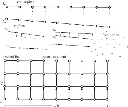
Square-Knowing-n Protocol: The initial leader L first computes √n on its line by any plausible algorithm and then expands its line to the right by attaching free nodes to make its length √n. Then it exploits the down ports to create a replica of its line. The replica has also length √nand has its own leader but in a distinguished stateLs. This new line plays the role of a seed that starts creating other self-replicating lines of length √n. In particular, the seed attaches free nodes to its down ports, until all positions below the line are filled by nodes and additionally all hori-zontal connections between those nodes are activated. Then it introduces a leaderLr to one endpoint of the replica and starts deactivating the vertical connections to release the new line of length√n. These lines withLr leaders are to-tally self-replicating, meaning that their children also begin in stateLr. The initial leaderL waits until the up ports of a non-seed replicar become totally aligned with the down ports of the square segment that has been constructed so far. So, initially it waits until a replica becomes attached to the lower side of its own line. When this occurs, it activates all intermediate vertical connections to make the construc-tion rigid, increments a row-counter by one (initially 0), and moves to the new lowest row. If at the time of attachment
Lr
Ls seed replica
replicas
L
Lr
Lr Lr
Lr
Lr
free nodes
square segment
√n original line
[image:8.612.59.284.53.240.2]Lr
Figure 2: The seed at the top has created another replica which has just been released in the solution. At the bottom appears the square segment that has been constructed so far. A replica has just arrived (from below) and will be attached to the segment.
will be nodes attached to the down ports ofr. Lreleases all these nodes, by deactivating the active connections ofr to them, and then waits for another non-seed replica to arrive. When the row-counter becomes equal to√n−1, the leader for the first time accepts the attachment of the seed to its construction and when the seed is successfully attached the leader terminates. This completes the construction of the √n
×√nsquare. See Figure 2 for an illustration.
The reason for attaching the seed last, and in particular when no further free nodes have remained, is that otherwise self-replication could possibly cease in some executions. Ob-serve also that we have allowed theL-leader to accept the attachment of a replica to the square segment even though the replica may be in the middle of an incomplete replica-tion. This is important in order to avoid reaching a point at which some free lines are in the middle of incomplete repli-cations but there are no further free nodes for any of them to complete. For a simple example, consider the seed and a replica r and √n free nodes (all other nodes have been attached to the square segment). It is possible that√n−1 of the free nodes become attached to the seed and the last free node becomes attached to r. We have overcome this deadlock by allowingLto accept the attachment ofrto the square segment. When this occurs, the free node will be released and eventually it will be attached to the last free position below the seed.
We now give, in Protocol 1, one of the possible codes for replicating the lines. We present a version that does not use the line’s leader in order to successfully self-replicate. A direct replication controlled by the leader is simpler to conceive but its code is lengthy (it can be found in the full paper). Without loss of generality, we assume that one line haseon both of its endpoints andion the internal nodes, and every (free) node is in state q0. The protocol works
as follows. Free nodes are attached below the nodes of the original line. When a node is attached below an internal nodei, both becomei1 and when a node is attached below
an endpointe, both becomee1. Moreover, adjacent nodes of
the replica connect to each other and every such connection increases their index, so that their index counts their degree. An internal node of the replica can detach from the original line only when it has degree 3, that is when, apart from its vertical connection, it has also already become connected to both a left and a right neighbor on the replica. On the other hand, an endpoint detaches when it has a single internal neighbor. It follows that the replica can only detach when its length (counted in number of horizontal active connections) is equal to that of the original line. To see this, assume that a shorter line detaches at some point. Clearly, such a line must have at least one endpoint that corresponds to an internal nodeijof the replica. But this node is an endpoint of the shorter line, so its degree is less than 3, i.e. j <3, and we conclude that it cannot have detached. To make the protocol also replicate the leader-state simply replace one
e withL, Ls, orLr and map it toLs, Lr, Lr, resp., in the replica, when detaching.
Protocol 1No-Leader-Line-Replication
Q={q0, e, e1, i, i1, i2, i3} δ:
(i, d),(q0, u),0→(i1, i1,1)
(e, d),(q0, u),0→(e1, e1,1)
(ij, r),(ik, l),0→(ij+1, ik+1,1) for allj, k∈ {1,2}
(i1, r),(e1, l),0→(i2, e2,1)
(i2, r),(e1, l),0→(i3, e2,1)
(e1, r),(i1, l),0→(e2, i2,1)
(e1, r),(i2, l),0→(e2, i3,1)
(i3, u),(i1, d),1→(i, i,0)
(e2, u),(e1, d),1→(e, e,0)
Lemma 2. There is a protocol (described above) that when executed onnnodes (for alln with integer√n) w.h.p. con-structs a√n×√n square and terminates.
4.3
Simulating a TM
We now assume as given (from the discussion of the pre-vious section) a √n×√n square with a unique leader L
i≤n−1 and therefore the length of its binary representa-tion|i|=O(logn), thus|(i, n)|=O(logn), but the available space is Θ(n) = Θ(2logn) = Ω(2|(i,n)|
) (still it is linear in the size of the whole shape to be constructed).
The protocol invokesndistinct simulations ofM, one for each of the pixelsi∈ {0,1, . . . , n−1}, beginning fromi= 0 and every time incrementingiby one. The leader maintains the current value of i in binary, in a pixel-counter pixel
stored in theO(logn) leftmost cells of the tape. Recall that the leader knowsnfrom the procedures of the previous sec-tions. So, we may assume that the tape also holds in advance
n and√n in binary (again in the leftmost cells). Initially
pixel = 0 and the leader marks the 0th node, that is the bottom left corner of the square. Then it simulatesM on input (pixel,√n). WhenM decides, if its decision isaccept, the leader marks the node corresponding topixelason, oth-erwise it marks it asoff. Then the leader incrementspixel
by one, marks the node corresponding to the new value of
pixel(which is the next node on the tape), clears the tape from residues of the previous simulation, invokes another simulation ofM on the new value ofpixel, and marks the corresponding node asonoroff according toM’s decision. The process stops whenpixel=n, in which case no further simulation is executed. When this occurs, the leader starts walking the tape in the opposite direction until it reaches the bottom left corner. In the way, it deactivates all con-nections involving at least oneoff node, leaving active only the connected 2D shape consisting of theon nodes.
The following theorem states the lower bound implied by the construction described in this section.
Theorem 2. LetL= (S1, S2, . . .)be a connected 2D shape
language, such thatLis TM-computable in spaced2. Then
there is a protocol (described above) that w.h.p. constructs
L. In particular, for all d ≥ 1, whenever the protocol is executed on a population of size n = d2, w.h.p. it
con-structs Sd and terminates. In the worst case, when Gd
(that is, the shape of Sd) is a line of length d, the waste is(d−1)d=O(d2) =O(n).
Remark 3. If the system designer knew n in advance, then he/she could preprogram the nodes to simulate a TM that constructs a specific shape of sizen, e.g. the TM corre-sponding to the Kolmogorov complexity of the shape. In this work,nis not known in advance, so we had to preprogram the nodes with a TM that can work for alln.
Remark 4. The above results can be immediately modi-fied to construct patternsinstead of shapes. The idea is to keep the same constructor as above and simulate TMs that for every pixel output a color from a set of colorsC.
Remark 5. In all the above constructions the unique lea-der assumption can be dropped in the price of sacrificing ter-mination. In this case, the constructions become stabilizing by the reinitialization technique, as e.g. in [12], but should be carefully rewritten.
4.4
Parallelizing the Simulations
We now present an approach for parallelizing the simula-tions. Assume that there is a TMM deciding each pixel in space k, that k and d are computable in space O(n), and thatn=k·d2.
The leader, instead of constructing a square, constructs now a spanning line of length d2, say in the x dimension,
corresponding to a linear expansion of the pixels of ad×d
square. Moreover, the leader creates a seed of lengthk−1 and uses it to partition the rest of the nodes into lines of lengthk−1 in theydimension. Each such line will be at-tached below one of the nodes of thex-line. When ally-lines have been attached, the leader, for all 0≤i≤d2
−1, ini-tializes the memory of the line attached below pixeliwith (i, d). Then all simulations of M are executed in parallel and eventually each one of them sets itsx-pixel to eitheron
oroff. When all simulations have ended, the leader releases the y-lines and then partitions the x-line into consecutive segments of lengthd (see Figure 3(a)). Each segment cor-responds to a row of thed×dsquare to be constructed. In particular, segment i≥1 (counting from left) corresponds to rowi(bottom-up). Moreover, ifiis even (odd), segmenti
should match with its upper (lower) side to the upper (lower) side of segmenti−1. The leader marks appropriately the nodes of each segment to make them aware of the orientation that they should have in the square. Moreover, it assigns a unique key-marking to each segment so that segmentican easily and locally detect segmenti−1. In particular, ifiis odd (even), it marks nodesiandi−1 of the segment count-ing from left to right (right to left); see Figure 3(b). Then the leader releases, one after the other, all segments. The segments are free to move in the solution until they meet and recognize their counterpart, and when this occurs the two segments bind together. Eventually, thed×dsquare is constructed and every pixel is in the correct position. The leader can detect this and release the constructed shape con-sisting of theonpixels.
5.
CONCLUSION AND OPEN PROBLEMS
There are several interesting open problems related to the findings of this work. A very intriguing problem is to give a proof, or strong experimental evidence (we have already some preliminary such evidence), that there is no analogue of Theorem 1 if all processes are identical (i.e. no unique leader). A possibility left open then would be to achieve high probability counting with f(n) leaders. There is also work to be done w.r.t. analyzing the running times of our protocols and our generic constructors and proposing more efficient solutions. Also it is not yet clear whether the proto-col of Section 3.1 is the fastest possible nor that its success probability or the upper bound onnthat it guarantees can-not be improved; a proof would be useful. Moreover, it is not obvious what is the class of shapes and patterns that the TMs considered here compute. Of course, it was sufficient as a first step to draw the analogy to such TMs because it helped us establish that our model is quite powerful. How-ever, still we would like to have a characterization that gives some more insight to the actual shapes and patterns that the model can construct.
A possible refinement of the model could be a distinction between the speed of the scheduler and theinternal opera-tion speed of a component. Such a distinction is very nat-ural, because a connected component should operate at a different speed than it takes for the scheduler to bring two nodes into contact. It would also be interesting to consider for the first time a hybrid model combining active mobility controlled by the protocol and passive mobility controlled by the environment.
pro-L 1 2 d
3
4 5
(a)
1 2 3 4 5
(b)
Figure 3: (a) d2 lines of lengthk
−1 each, are pendent below thed2 pixels. The pixels are arranged linearly in dimensionxand have been partitioned into equal segments of lengthdeach (see the black delimiters). (b) The segments have been released in the solution, and now they have to gather together and form the square.
posed here) that take other real physical considerations into account. In this work, we have restricted attention on some geometrical constraints. Other properties of interest could be weight, mass, strength of bonds, rigid and elastic struc-ture, collisions, and the interplay of these with the interac-tion pattern and the protocol. Moreover, in real applicainterac-tions mere shape construction will not be sufficient. Typically, we will desire to output a shape/structure thatoptimizes some global property, like energy and strength, or that achieves a
desired behavior in the given physical environment.
Finally, it would be interesting to develop routines that can rapidly reconstruct broken parts. For example, imagine that a shape has stabilized but a part of it detaches, all the connections of the part become deactivated, and all its nodes become free. Can we detect and reconstruct the broken part efficiently (and without resetting the whole population and repeating the construction from scratch)? What knowledge about the whole shape should the nodes have in order to be able to reconstruct missing parts of it?
Acknowledgments: The author would like to thank D. Amaxilatis and M. Logaras for implementing (in Java) the counting protocol of Section 3.1 and experimentally verifying its correctness and also D. Doty for a few fruitful discussions on the same protocol at the very early stages of this work.
6.
REFERENCES
[1] D. Angluin, J. Aspnes, Z. Diamadi, M. J. Fischer, and R. Peralta. Computation in networks of passively mobile finite-state sensors.Distributed Computing, pages 235–253, March 2006.
[2] D. Angluin, J. Aspnes, and D. Eisenstat. Fast computation by population protocols with a leader.
Distributed Computing, 21(3):183–199, September 2008.
[3] J. Aspnes and E. Ruppert. An introduction to population protocols.Bulletin of the European Association for Theoretical Computer Science, 93:98–117, October 2007.
[4] D. Doty. Timing in chemical reaction networks. In
Proc. of the 25th Annual ACM-SIAM Symp. on Discrete Algorithms (SODA), pages 772–784, 2014. [5] P. Ehrenfest and T. Ehrenfest-Afanassjewa. ¨Uber zwei
bekannte einw¨ande gegen das boltzmannsche h-theorem.Phys.Zeit., 8:311–314, 1907.
[6] W. Feller.An Introduction to Probability Theory and Its Applications, Vol. 1, 3rd Edition, Revised Printing. Wiley, 1968.
[7] S. C. Goldstein, J. D. Campbell, and T. C. Mowry. Programmable matter.Computer, 38(6):99–101, 2005. [8] R. Guerraoui and E. Ruppert. Names trump malice:
Tiny mobile agents can tolerate byzantine failures. In
36th International Colloquium on Automata, Languages and Programming (ICALP), volume 5556 ofLNCS, pages 484–495. Springer-Verlag, 2009. [9] M. Kac. Random walk and the theory of brownian
motion.American Mathematical Monthly, pages 369–391, 1947.
[10] O. Michail, I. Chatzigiannakis, and P. G. Spirakis. Mediated population protocols.Theoretical Computer Science, 412(22):2434–2450, May 2011.
[11] O. Michail, I. Chatzigiannakis, and P. G. Spirakis.
New Models for Population Protocols. N. A. Lynch (Ed), Synthesis Lectures on Distributed Computing Theory. Morgan & Claypool, 2011.
[12] O. Michail and P. G. Spirakis. Simple and efficient local codes for distributed stable network
construction. InProceedings of the 33rd ACM Symposium on Principles of Distributed Computing (PODC), pages 76–85. ACM, 2014.
[13] O. Michail and P. G. Spirakis. Terminating population protocols via some minimal global knowledge
assumptions.Journal of Parallel and Distributed Computing (JPDC), 81:1–10, 2015.
[14] P. W. Rothemund. Folding dna to create nanoscale shapes and patterns.Nature, 440(7082):297–302, 2006. [15] M. Rubenstein, A. Cornejo, and R. Nagpal.
Programmable self-assembly in a thousand-robot swarm.Science, 345(6198):795–799, 2014.
[16] J. L. Schiff.Cellular automata: a discrete view of the world, volume 45. Wiley-Interscience, 2011.
[17] D. Woods, H.-L. Chen, S. Goodfriend, N. Dabby, E. Winfree, and P. Yin. Active self-assembly of algorithmic shapes and patterns in polylogarithmic time. InProceedings of the 4th conference on Innovations in Theoretical Computer Science, pages 353–354. ACM, 2013.
[18] M. Zakin. The next revolution in materials.DARPA’s 25th Systems and Technology Symposium
[image:10.612.69.538.52.173.2]