Towed-Array Calibration
Malcolm John Goris
BE (Elec) Hons I
A thesis submitted for the degree of
Doctor of Philosophy of
The Australian National University
•••
III
Preface
I am sincerely grateful to all those who provided valuable assistance and support throughout my PhD; in particular, to Dr. Donald McLean and Dr. Iven Mareels for their support, guidance and helpful discussions and to Mr. Ralph Marson, Dr. Rene Grognard and Prof. Doug Gray for their helpful discussions.
I acknowledge the Australian Commonwealth Government for funding the activities of the Cooperative Research Centre for Robust and Adaptive Systems under the Cooperative Research Centres program. For providing the financial assistance to pursue PhD studies I thank the Australian Commonwealth Government and the Cooperative Research Centre for Robust and Adaptive Systems. I appreciate the CSIRO Division of Radiophysics for their encouragement to take up postgraduate studies.
Above all, I thank my wife Kathleen for her love and encouragement.
Statement of Originality
This thesis describes work carried out between 1992 and 1995 under the guidance of Dr. Donald McLean of the CSIRO Division of Radiophysics and Dr. Iven, Mareels of the Australian National University. Except where acknowledged, the work presented in this thesis is my own.
Publications
~
Malcolm J. Goris December 18, 1995
~
Part of the work done for this thesis has been published as listed below.
Journal Papers
[Jl] M. J. Goris and D. J. McLean, "Towed Array-Shape Estimation - Least Square Error Method", submitted to IEEE 1. Ocean. Eng., 1995
[J2] M. J. Goris, D. J. McLean and I. Y. Mareels, "Array-Shape Estimation Using Signal Information", submitted to IEEE Trans. Information Theory, 1995
•
IV
[14] M. J. Goris and D. A. Gray, ''Reducing the Computational Load of a Kalman Filter when there are more Measurements than States", submitted to Int. 1. Systems Science, 1995
Conference Papers
[C1] M.1. Goris and D. J. McLean, "Calibrating a Towed Array Using Redundant Information from an Impinging Broadband Signal", Int. Con! on Sig. Proc. and Applic. Tech., 1995 [C2] D. A. Gray and M. 1. Goris, "A Kalman Filter Based Data Fusion Approach for Estimating
the Shape of a Towed Sonar Array", Int. Conf. on Neural Networks and Sig. Proc., 1995
Technical Reports
[T1] M. J. Goris and D. J. McLean, ''Towed Array-Shape Estimation - A Comparison of Methods", 1995
v
Abstract
Array processing techniques, such as beamforming, require accurate knowledge of the positions of the array's sensors. If the array's shape is not known accurately enough the array processor will be unable to estimate the signal parameters it was designed to. Towed arrays have omnidirectional sensors called hydrophones that are built into a thin flexible cylinder. The cylinder, drawn behind a towing vessel, is often assumed to have a linear shape. This assumption may not be true due to maneuvering of the tow vessel, ocean currents and hydrodynamic effects. To maintain the processor's performance under these conditions the array must be calibrated by regularly estimating its shape.
In this thesis I investigate methods of towed-array calibration. The investigation includes a theoretical derivation of the necessary conditions for array calibration using signals, development of algorithms and a comparison of algorithms from the literature.
I show the conditions necessary to determine the array and signal parameters using information only from impinging signals. This is a fundamental question of invertibility and applies to any type of array. I relate these results to the more specific problem of towed arrays which have additional geometric constraints on their shape.
I describe three new algorithms for estimating the shape of towed arrays. Two of the algorithms use signal information only. The third algorithm uses a state-space representation of the array that combines signal and heading-sensor information, and uses a model of the dynamics of towed, flexible cylinders.
•
Vl
Preface
Abstract
List of Figures
List of Tables
Glossary Chapter 1 1.1 1.2 1.3 1.4 Chapter 2 2.1 2.2 2.3 2.3.1 2.4 2.5 Chapter 3 3.1 3.2 3.2.1 3.2.2 3.2.3 3.2.4 3.3 3.4
Contents
IntroductionProblem Setting
Literature Overview .
Contributions .
Thesis Outline
Array Processing
. Hydrophone Signals.
Narrowband Signals .
Array-Covariance Matrix . .
...
III v x XlV XV 1 3 5 6 6 9 9 12 12Signal model - deterministic or random? . . . . . . . . . . .. 14 Beamforming. . . . . . . . 14 Geometric Constraints and the Chord Approach. 16
Inverting the Spatial Correlation Function 20
Problem Description and Background . . . 20
Uniqueness of the Factorisation of the Array-Covariance Matrix. 23
Observability of noise. . . . . . . . . . . . . . . .. 23 Observability of signal and sensor parameters when the signals are incoherent and noise is spatially uncorrelated. . . . . . 24
Observability of signal and sensor parameters when the signals are coherent and there is one signal source. . . . . . . . . . . 35 Observability of signal and sensor parameters when the signals are
coherent and there is more than one signal source. .. . . 40
•
•
vzz
Chapter 4 New Array Calibrators 44
4.1 Enter the Calibrators . . . .. 44
4.2 A Narrowband Self Calibrator. . . . . . . . . . . .. 45
4.2.1 Theory . . . . . . .. 46
4.2.2 Examples . . . . . . . . .. 47
4.2.3 Summary of the narrowband self calibrator . . . .. 51
4.3 A Broadband Self Calibrator . . . . . . . . .. 51
4.3.1 Estimating the relative time of arrival of the calibrating signal .. 51
4.3.2 Example . . . 53
4.3.3 Summary of the broadband self calibrator . . . .. 54
4.4 Data Fusion Using Kalman Filters . . . 55
4.4.1 Towed arrays in (state) space . . . 57
4.4.2 Examples and discussion . . . .. 63
4.4.3 Extensions to the state-space system . . . .. 68
4.4.4 Reducing computational load when there are more measurements than states . . . . . . . . 71
4.4.5 Summary of the Kalman-filter-based array calibrator . . . .. 73
Chapter 5 Comparison of Algorithms 75 5.1 Introducing the Self Calibrators . . . .. 75
5.2 The Calibrators Explained . . . .. 76
5.2.1 A time-domain method . . . .. 77
5.2.2 Phase difference self-survey (PDSS) .. . . . .. 77
5.2.3 A least-squares error method . . . 78
5.2.4 Self-cohering method . . . 78
5.2.5 Redundant self-calibration method . . . 79
5.2.6 Eigenvector method . . . 81
5.2.7 A maximum-likelihood approach . . . .. 82
5.2.8 Sharpness method . . . 83
•
••
VIII
5.3
5.3.1
Simulations and Results . . . . . . . . "
84-TIme-domain method . . . . . . 88
5.3.2 Phase difference self-survey (PDSS) .. . . . . . . . .. 89
5.3.3 Least-squares error method. . . . . . . . .. 90
5.3.4 Self-cohering method . . . .. 90
5.3.5 5.3.6 Redundant self-calibration Eigenvector method . . . . 90 91 5.3.7 Maximum-likelihood (rvIL) approach. . . . . . . . . . . . . .. 92
5.3.8 Sharpness method . . . . . . . . . . . . . . . .. 93
5.3.9 Continuous simulation with beamformer output. . . .. 93
5.4 Chapter 6 6.1 6.2 6.3 6.3.1 Conclusions and Summary of Chapter 5 . . . . . . . . . . .. 94
Applying Sharpness to Towed Arrays 96 Sharpness Revisited . . . . More Array Concepts . . . . . . . . . 96 97 Development of the Sharpness Concept . . . . . .. 99
Sharpness applied to optical astronomy. . . . . . 99
6.3.2 Proof of the sharpness function and comparison with radio astronomical methods of self-calibration . . . .. 100
6.3.3 6.3.4 6.4 6.5 6.6 Chapter 7 7.1 7.1.1 Sharpness applied to towed arrays . . . Mathematical analysis of sharpness . . . 101 103 Why Sharpness Works . . . . . . . . . . . . . . . 104
New Sharpness Functions for Towed-Arrays . . . 109
Summary of Chapter 6 Conclusion Further Research. . Data modelling. . . · 112 114 · 115 . . . . 115
7.1.2 Three-dimensional array calibration . . . . . . . . . . . . . . . 116
7.1.3
7.1.4
7.1.5
Bibliography
Issues on array-calibration accuracy . . . .
Processing by subarrays . . . .
Development of real-time calibrators . . . .
· 116
· 116
· 117
•
lX
Appendix A In factorising R = ARsA H
+
J, all possible solutions for A must have the same rank and exist in the same subspace ofeM.
128Appendix B Simultaneous solution of sensor positions from the steering-vector
matrix for three sensors and three signals.
129
Appendix C The derivatives of sharpness function S2 with respect to array-shape
parameters {a A} and {f3 A}. 130
x
Figure 1
Figure 2
Figure 3
Figure 4
Figure 5
Figure 6
Figure 7
Figure 8
List of Figures
Definition of coordinate system. . . . . . . . 9
Projection of sensor position onto the direction cosine vector. .
Schematic of a delay and sum beamformer. . . .
Images from a uniform, 7-sensor array using a conventional beamformer
11
15
(dashed line) and a Capon estimator (solid line). . . . . 16
Model of the segmented array approximation. . . . . . . . . . . . . . . 17
Choose the solution closest to the tow-vessel's path. . . . . . . . 18
Estimating signal direction using two hydrophone pairs with heading sensors. 18
Translations (b), rotations (c) and reflections (d) are regarded as trivial
duplications of the one solution (a) . . . 21
Figure 9 A linear combination of two steering vectors will be a steering vector only if
all sensors lie on two parallel lines whose direction bisects the DOAs of the
two signals. . . . . . . . . . 25
Figure 10 Given two signal-source DOAs, t:lle sensor positions can be found as the .
intersection of two sets of wavefronts, which are at distances of dml and dm2
from the reference point. . . . . . . . . . . . . . . . . . . . . . . . . . . . 26
Figure 11 Basic system, with 3 signals and 3 sources. The intervals XI-X2 and XI-X3
are the diameters of circles upon which the points, at distances {dmn } from the origin in the direction of the signals, {8n }, must lie . . . 27
Figure 12 The first guess for X2 is incorrect because d3383 lies outside the circle defined
by Xl, d3181 and d3282 . . . . . • . . . 28
Figure 13 The second guess for X2 is incorrect because d3383 lies inside the circle
defined by Xl, d3I8I and d3282 . . . . . . . 28
Figure 14 The first three sensors define the signal DOAs so that for any other sensor the
perpendiculars from the lines defined by the direction cosines, {8n }, at the
points defined by {dmn } must intersect at a common point . . . . . . . . . . . 30
Figure 15 Given amI and {sn}, then am2 and am3 can be found from the intersection of
two circles with radii
IS21
andIS31. .
. . .
.
. ...
37Figure 16 Plot of typical function f(dml ). . . . . . 38
Figure 17 Two equivalent systems have array shapes shown by the solid line and the
circles, respectively . . . 39
Figure 18 Resolving the twin ambiguity when (a) signal DOA is greater than the angle
Figure 19 Figure 20
Figure 21 Figure 22 Figure 23 Figure 24
Figure 25 Figure 26
•
Xl
Actual and estimated array shapes. Source direction is 90°. . . . . . . . . .. 48
Normalised hydrophone position errors at each hydrophone. Source direction is 90° . . . 48
Actual and estimated array shapes. Source direction is 10°. . . . . . . .. 49
Block diagram of a generalised cross correlator. . . . . . . .. 53
Actual (solid line) and estimated (dashed line) array shapes. . . . . . . . .. 54
Capon estimator images for assumed straight (dashed line) and calibrated (solid line) arrays. . . . . . . . . . . . . . . . 54
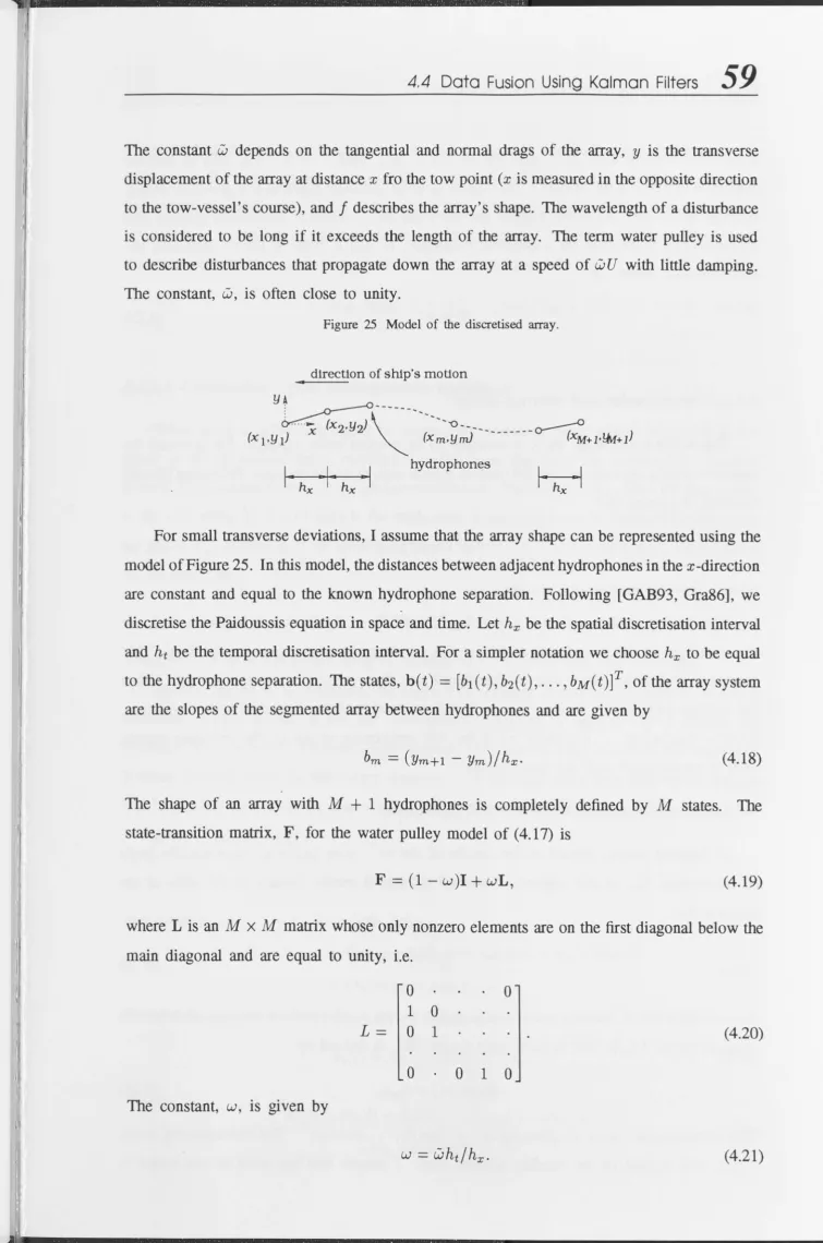
Model of the discretised array. . . . . . . . .. 59
Mean square errors of the Kalman filter for (a) calibrating-signal measurements only, (b) heading-sensor measurements only and (c) calibrating-signal and heading-sensor measurements combined. SNR=- 2OdB, a q2 = 0.05 and DOA=90° . . . 64
Figure 27 MSE of the Kalman filter state estimates using a calibrating signal with DOA of (a) 90°, (b) 45°, (c) 10° and (d) 0°. SNR is -20 dB . . . 65
Figure 28 MSE of the Kalman filter state estimates using a calibrating signal with SNR of (a) -20 dB, (b) -25 dB, (c) -30 dB and (d) -35 dB. DOA is 90° . . . 66
Figure 29 MSE of the Kalman filter state estimates using heading sensors with process noise variance of (a) 0.05 and (b) 0.1. . . . 67
Figure 30 MSE of the state estimates when the DOA is known exactly (solid line) and when DOA estimate is used in place of its true value (dashed line). (a) ~ ~ </>=80°, </>=90°, (b) </>= 10°, </>=20°. . . . . 68
Figure 31 Typical frequency wavenumber diagrams for an array with 128 hydrophones and two signal sources; (a) array is linear, and (b) array has sinusoidal shape with an amplitude of 0.50 metres in the direction orthogonal to ship's motion .. 79
Figure 32 Tillle taken to estimate array shape from 1024 samples of raw data. . . . .. 87
Figure 33 Array calibration results - actual array shape (solid line) estimated array shape (asterisks); (a) time-domain method, scenario 3; (b) PDSS method, scenario 6; (c) self-cohering method, scenario 8; (d) redundant self-calibration method, scenario 6; (e) eigenvector method, scenario 19; Cf) maximum-likelihood method, scenario 11; (g) maximum-likelihood method, scenario 12; (h) sharpness method, scenario 1. . . . . . . . . . . 88
Figure 34 Detail of a typical cross correlation with two signal sources. . . . 89
• •
Xll
Figure 36 Array calibration results for scenario 1; sharpness method. Continuous and
dashed lines represent uncalibrated and calibrated beamformer output
respectively. . . . . 93
Figure 37 Continuous simulation - ideal beamformer output.. . . . . .. 94 Figure 38 Continuous simulation, (a) time-domain method, (b) PDSS method, (c)
least-squares error method, (d) self-cohering method. . . . . 95
Figure 39 Continuous simulation, (a) redundant self-calibration method, (b) eigenvector
method, (c) maximum-likelihood method, (d) sharpness method . . . 95
Figure 40 Pupil and transfer functions of a telescope. . . .. 98
Figure 41 Muller and Buffington's [1] model for atmospheric phase disturbances. The position of the arrows indicates relative phase. Phase errors are independent
of signal direction, assuming that all signals are located in an isoplanatic patch
of the sky. . . . . 100
Figure 42 Flow chart for basic operation in the maximisation of sharpness, S2. One
iteration loop consists of doing the basic flow chart operation for every
parameter, {a,\} and {/h}. Sharpness is maximised by repeating the iteration loop a fixed number of times. . . . . . . . . 102 Figure 43 Relative values of sharpness versus estimated sensor separation. The system has
two sensors with a true separation of one and a single signal at 90°. The value
for sharpness is given relative to the sharpness at the correct separation. . . 105 Figure 44 Example of an unparameterised array. . . . 106
Figure 45 Contour plot of sharpness versus the estimated second and third segments'
angular deviations. The array has four sensors, with a true array shape defined
by the point A. The nearest local maximum to A is point B. The signal DOAs
are (a) 90°, (b) 90° and 150°, and (c) 90° and 100°. . . . . . . . . . . . . 107 Figure 46 Plot of actual (solid lines) and estimated (dashed lines) array shapes and
beamformer images using sharpness function S2. The array is not
parameterised in (a), (c) and (e). The array is modelled as the sum of three sinusoids with wavenumbers of H /2, H and 2H in (b), (d) and (f). . . 109 Figure 47 Sharpness versus simulation number. The solid line is for a nominal standard
deviation of 5°, and the dashed line is for a nominal standard deviation of
10°. (a) ideal, convex sharpness function, and (b) sharpness function S2.. 111 Figure 48 Results of simulation tests for convexity of trial sharpness functions. A
performance indicator value of 100% indicates that the function is convex in a
• ••
[image:12.814.27.797.18.1088.2]Xlll
Figure 49 Plot of actual and estimated array shapes and beamformer images (estimates are shown with dashed lines) using trial function 9. The array is unconstrained in (a) and (c). The array is modelled as the sum of three sinusoids with
wavenumbers of H /2, H and 2H in (b) and (d) . . . .. 112 Figure 50 Example of how a towed array's shape may vary during a tow-vessel
•
XlV
Table 1
Table 2
Table 3
Table 4
Table 5
Table 6
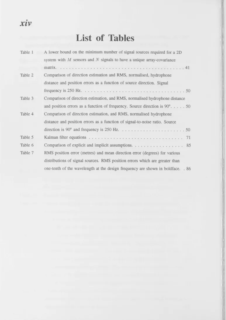
Table 7
List of Tables
A lower bound on the minimum number of signal sources required for a 2D
system with M sensors and N signals to have a unique array-covariance
matrix. . . . .. 41
Comparison of direction estimation and RMS, normalised, hydrophone
distance and position errors as a function of source direction. Signal
frequency is 250 Hz. . . 50
Comparison of direction estimation, and RMS, normalised hydrophone distance
and position errors as a function of frequency. Source direction is 90° . . . 50
Comparison of direction estimation, and RMS, normalised hydrophone
distance and position errors as a function of signal-to-noise ratio. Source
direction is 90° and frequency is 250 Hz. . . 50
Kalman filter equations . . . .. 71
Comparison of explicit and implicit assumptions. . . .. 85
RMS position error (metres) and mean direction error (degrees) for various
distributions of signal sources. RMS position errors which are greater than
[image:13.816.19.792.17.1109.2]xv
Glossary
List of Symbols and Functions
(
...
) A an amn BW Cs dm dmnOn
Oq;,B
fo H A M N Pb
CPn
R Rn Rs p Tjk T(X)sn(
t
)
s(t)
t
T
()n
tmn Vm (t)
time average
matrix of phase changes, amn
vector of phase changes, amn , for the nth signal; steering vector
phase change of the nth signal at the m th hydrophone
bandwidth
speed of sound in water
distance from the m th hydrophone to the first in the line of sight to the calibrating
signal
distance from the m th hydrophone to the first in the line of sight to the nth
signal
direction cosine vector of the nth signal
direction cosine vector for the look direction
cp, ()
centre frequency of a signal
Hermitian transpose
wavelength
number of hydrophones
number of impinging signals
beamformer power
azimuth direction of arrival of the nth signal
array-covariance matrix
noise-covariance matrix
signal-covariance matrix
distance between hydrophones
correlation between the jth and kth sensors
spatial correlation function
nth analytic signal as a function of time
vector of all impinging signals as a function of time
time
matrix transpose
elevation direction of arrival of the nth signal
•
XVl
v( t) vector of all noise as a function of time
X m posi tion of the m th hydrophone
Xm position of the m th hydrophone in the x-direction
Ym position of the mth hydrophone in the y-direction
Zm position of the m th hydrophone in the z-direction
Zm (t) anal ytic signal at the m th hydrophone as a function of time
z ( t) vector of all hydrophone signals as a function of time
List of Acronyms
2D
two dimensional3D
three dimensionalDOA
direction of arrivalLSE
least -squares errorML maximum likelihood
MSE
mean-square errorPDSS
phase difference self surveyRMS
root mean squareSNR
signal-to-noise ratioTDOA
time delay of arrivalChapter 1 Introduction
Towed arrays have omnidirectional, underwater, acoustic sensors called hydrophones that are built into a thin, flexible cylinder. The cylinder is drawn behind a towing vessel, such as a ship or submarine. Towed arrays are used in seismology for mineral exploration and in passive sonar surveillance where it is desirable to detect another vessel without revealing the tow-vessel's own location. Array processors combine the signals from the hydrophones to estimate signal parameters such as direction of arrival (DOA), power, spectrum and range to the source. For a correctly calibrated array, the signal-to-noise ratio (SNR) improvement of the array over one of its sensors is proportional to the number of sensors in the array and the resolution and range-estimation accuracy improves with the length of the array. And so, because of the need for increased resolution and SNR, users demand longer arrays with more hydrophones. Towed arrays are now of the order of one kilometre in length.
Towed arrays are often assumed to be linear when the tow vessel travels in a straight line. However, this assumption may not always be true due to ocean currents and hydrodynamic effects. A linear array is able to resolve the DOA angle relative to itself but an ambiguity exists as to where on the cone defined by that angle the signal source really is. If the signal source is assumed to lie on a plane the ambiguity becomes whether the signal source is on the left or the right side. This ambiguity is resolved by turning the tow vessel and noting in which direction the signal source has moved. During the turn the array will have a bend in it. At typical tow speeds of around 5 knots up to six minutes (for a one kilometre array) can elapse before the array regains its nominal, linear shape.
Array processing techniques require accurate knowledge of the positions of the array sensors [Car79, Has84, Nie91]. Without sufficiently accurate sensor-position knowledge an array processor will be unable to estimate the signal parameters it was designed to. The sensitivity of an array processor to incorrect knowledge of the sensor locations depends on the complexity of the processor. For example, high resolution, eigenvector-based direction-of-arrival estimators [JD82, Pi189], range estimators [Hin79, Has84], and adaptive noise cancellers [Ows84b] are very sensitive to imperfect sensor-location knowledge.
2
Chapter 1 Introductionperformance of the array processor and to allow processing to continue during a maneuver the
locations of the hydrophones need to be estimated each time the array is to be processed. This
is commonly called array calibration or array straightening. The term "array calibration"
generally implies knowing the array's shape, gain characteristics of the hydrophones and
amplifiers and properties of the propagating medium. In this thesis it is assumed that the
gain characteristics of the sensors are known and that the propagating medium is uniform and
lossless. And so, to calibrate a towed array we need estimate only its shape. Care needs to
be taken when reading the literature on array calibration. For certain arrays it is implicit in
the problem definition that the array shape is known accurately and calibration means knowing
only the channel gains. Radio astronomy arrays are one example; the sensors are directional
(unlike hydrophones which are omni-directional) and atmospheric disturbances cause unknown
channel-related gains that are assumed to be independent of the signal-source distribution. TIlis
definition of calibration is not applicable to towed arrays.
One approach to towed-array calibration is to instrument the array with a number of heading
and depth sensors. For mechanical and economical reasons the numbers of heading and depth
sensors are often small which are not enough to infer the location of every hydrophone directly.
Instead, the heading and depth sensors are used to estimate the coefficients of a low-order
polynomial approximation of the array shape [Ows81, Ows84a]. The advantages of heading
and depth sensors are that they provide shape information independently of external factors and
they are accurate. Their accuracy is on the order of 10
and they have a slowly varying bias also
on the order of 10
[Ows81]. The disadvantage of heading sensors is that they are expensive.
A second approach to array calibration is to use redundant information in the impinging
signals to estimate the array shape [GWR89, TN88, Wah93]. A typical signal-based calibrator
uses phase- or time-delay information from calibrating signals and estimates the hydrophone
locations by imposing geometric constraints. If the calibrating signals are the same ones whose
parameters are to be estimated then this is known as self calibration. This thesis deals largely
with self-calibration methods and in part with the combination of data from self calibrators
and heading sensors. Signals used for self calibration of towed arrays are assumed to be
uncooperative. That is, there is no control over their DOA or spectrum and they can't be turned
on and off as desired.
Array processors make use of correlations. The correlations are measured between pairs
of sensors. The spatial separation between sensors is known as the baseline over which the
correlation is measured. The correlations are functions of signal and noise parameters and
spatial separation. Array processors estimate the signal parameters given the correlations as a
7. 7 Problem Setting
3
a towed-array self calibrator estimates the sensor positions without knowledge of the signal
parameters. Once the array has been calibrated the array processor then estimates the desired
signal parameters. Estimating the sensor positions and signal parameters from the correlations
is an inverse problem; i.e. knowing correlation as a function of separation, what is separation
as a function of correlation?
Inverse problems are notoriously difficult. Towed-array self calibration is akin to finding
the discrete Fourier transform of a signal from discrete samples without knowing the times at
which the samples were taken. From this description, it is not obvious that the correlation
function will be invertible. A proof of the existence of the inverse and the conditions under
which it does is the first topic of this thesis.
However, the proof is necessary but not sufficient for practical applications. Although the
correlation function is invertible, this does not indicate whether the inversion is well posed. A
proof of invertibility is based on exact knowledge of the function (in our case, the correlations).
In practice, the correlations are not known exactly and must be estimated in the presence of
noise. Any algorithm that solves for the sensor and signal parameters will be sensitive, in some
degree, to the noisy correlation estimates. An algorithm necessarily makes certain assumptions
about the signals and noise. In practice the assumptions may not be entirely accurate. I discuss
how sensitive an algorithm is to deviations from the assumed conditions and how robust it is
to adverse conditions such as noisy correlation estimates.
I mentioned two approaches to towed-array calibration: sensor based and signal based. A
third possibility is to combine the two approaches. Combining sensor and signal information
will result in more accurate calibration. Problems to be overcome with this approach include
synchronising data, proper weighting of data according to the accuracy of the individual
measurements and combining the two measurement systems in an efficient framework.
1.1 Problem Setting
For the purpose of self calibration, the SNR of underwater acoustic signals can vary, as
a guide only, from -20 dB to 10 dB. The range to the signal source and the type of vessel
generating the signal affect the SNR; a merchant ship produces a lot of acoustic energy while
a submarine is designed to produce very little. The spectra of vessel-generated signals are
strongest at frequencies in the range of tens to hundreds of hertz [Coa90]. There are strong
spectral lines at the frequencies of rotating machinery, such as the engine's and propeller shaft's,
with harmonics at the propeller blade rate. Signal processing can be done in a broadband or
narrowband context. Broadband processing can be used to obtain a spectral signature of a signal
7.2 Literature Overview
5
1.2 Literature Overview
'This section presents a very general and incomplete overview of the literature with emphasis
on the more significant towed-array research. A more complete review is given in Chapter 5
which compares eight self calibrators with theory and computer simulation.
The dynamic behaviour of towed, thin, flexible cylinders was investigated by Paidoussis
[pai66a, Pai66b, Pai73a, Pai73b]. Paidoussis gave a differential equation describing the motion
of a towed cylinder in response to tow-point induced motion. The differential equation was
examined under special cases by Kennedy [Ken81], Kennedy and Strahan [KS81] and Ortloff
and Ives [0169]. Dowling examined the same special cases using a corrected version of
Paidoussis' equation [Dow88a, Dow88b]. In a Kalman-filter calibrator [GAB88, GAB93],
Gray et al. took advantage of a special form of the Paidoussis equation, valid for low-frequency
disturbances, known as the water-pulley model. 'This Kalman-filter calibrator is significant
because it uses the entire measurement history to calibrate the array as opposed to only the most
recent measurements. No other known algorithms make use of the array's dynamic behaviour.
The measurements in the Kalman-filter calibrator come from heading sensors.
Other heading-sensor-based calibrators have been developed by Owsley [Ows81, Ows84a].
The heading sensors are used to estimate a low order polynomial approximation of the array
shape. The slowly varying heading-sensor biases are also estimated.
Self calibration has been a concern of astronomers for longer than it has been for sonar
processors. Bucker [Buc78] and later Ferguson [Fer90b] adapted a technique known as
sharpness for towed-array calibration. Sharpness was originally used to correct, in real time,
atmospherically-distorted optical telescope images [MB74]. Sharpness was proven [HON77] to
be identical to another self-calibration algorithm that makes use of redundant baselines [MM92].
A number of array calibrators rely on the assumption that there is only one narrowband
signal impinging upon the array at a particular frequency or at a particular time (known as
disjoint source assumption) [GWR89, Dor78, WRM94, AGP93, 11M92]. This signal is called
the calibrating signal. The calibrators are sensitive, in varying degrees, to the disjoint source
assumption. Phase information from the calibrating signal is used to estimate the locations of
the array's hydrophones.
Some calibrators use the eigenstructure of the array-covariance matrix [LM87, FW88]. They
begin by estimating the number of signals that are represented in the array-covariance matrix.
This non-trivial task relies on the relative magnitudes of the eigenvalues. An iterative scheme
6
Chapter 1 Introductionfrom a number of problems. They are sensitive to the presence of coherent signals and to low SNR and they have a large computational load.
A few array calibrators assume the availability of broadband signals with which to calibrate an array [TN88, Wah93]. They use time-delay estimates to estimate the locations of the array's hydrophones. Time-delay estimation is insensitive to coherent and interfering signals but tends to be more sensitive to noise than some of the narrowband calibrators.
1.3 Contributions
The thesis contributes the following knowledge on towed-array calibration:
1. A proof of the fundamental question of the invertibility of the spatial correlation function (Chapter 3). I p~ove this for generic arrays and also relate the results to the more specific case of towed arrays.
2. Closed-form solutions for the sensor positions and signal DOAs from signal phase or time-delay information for both 2D and 3D arrays (Section 3.2.2).
3. Three new towed-array calibrators, including on~ that makes simultaneous use of both heading-sensor and signal data (Chapter 4).
4. A method for reducing the number of computations of a Kalman Filter when there are more measurements than states (Section 4.4.4).
5. Analysis and comparison, using computer simulations, of a selection of towed-array calibrators from the literature (Chapter 5). I show how robust the calibrators are to signal-source distributions and noise. I show how sensitive they are to their underlying assumptions.
6. A new sharpness function that can be maximised to calibrate a towed array. This was found after analysing the sharpness algorithm (Chapter 6).
1.4
Thesis Outline
1.4 Thesis Outline
7
In Chapter 3 I give the conditions under which the spatial correlation function will be
invertible. The analysis is applicable to generic arrays, for which only general sensor location
information is known a priori. Similar analyses have been done in [RS87a, RS87b, Lo92].
The thesis generalises these analyses and clarifies a number of the results. The proofs are more
intuitive than the ones given in [RS87a, RS87b, Lo92] as they are geometric rather than purely
algebraic. In addition they yield closed form solutions for the sensor locations and signal DOAs
from the phase-delay information. Based on the geometric constraints of Section 2.5, I infer
the conditions for which sensor and signal parameters will be unique for towed arrays.
I give three new array-calibration algorithms in Chapter 4. Two of the algorithms use a
least-square error optimisation. One uses a narrowband signal to estimate phase delays, and the
other uses a broadband signal to estimate time delays. The broadband algorithm is insensitive to
the presence of interfering and coherent signals. The third algorithm is based on a state-space
model of the array shape that includes a model of the array's dynamic motion. The model
allows signal and heading-sensor information to be combined easily. The states of the model
define the array's shape and a Kalman filter is used to estimate the states. I use computer
simulations to verify the theory.
In Chapter 5 I compare a number of representative array calibrators from the literature.
They were chosen on the basis that all calibrators in the literature are similar to one of the
representative calibrators. I identify the explicit and implicit assumptions made for each
calibrator. Computer simulations are used to investigate the sensitivity of the calibrators
to the underlying assumptions. I investigate how robust the calibrators are to variations in
the distribution of signal sources and in the array shape. I found that broadband calibrators
outperform narrowband calibrators in the presence of coherent signals.
Confiicting reports have been given concerning an algorithm known as sharpness. Bucker
[Buc78] and Ferguson [Fer90b] report that the sharpness algorithm is an effective towed-array
calibrator. Davidson and Cantoni [DC92] analyse sharpness algebraicly and show that the
sharpness algorithm will work only in special cases and is generally unusable for towed arrays.
In Chapter 6 I resolve the discrepancies between these reports. I investigate sharpness as
it is applied to towed arrays and compare it with the original sharpness algorithm which
was applied to optical telescopes. The sharpness algorithm is unique amongst signal-based
calibration algorithms. It ostensibly makes no assumptions about the signals. Further, it is
conceivable that it can be used to estimate parameters other than the array shape; the range
to the signal sources, for example. Simulations reveal new sharpness functions that give more
8
Chapter 1 IntroductionThe final chapter summarises the thesis and discusses the merits of various algorithms. I
Chapter 2 Array Processing
This chapter gives expressions for the hydrophone signals. I introduce the travelling-wave
model of the signals and the array-covariance matrix. I use the same model of the array and
signals as given in [Pi189]. The derivations for 2D arrays are essentially the same as for 3D
arrays, the only difference being in the size of the vectors that describe the sensor positions and
signal DOAs. In Chapter 3, 2D and 3D arrays are dealt with as separate cases. In the remaining
chapters the array and all signal sources are assumed to lie in a horizontal plane.
2.1 Hydrophone Signals
In this section I make no assumption about the bandwidth of the signals. Assume that the
signals impinging upon the array have an, as yet, unspecified bandwidth with centre frequency
fo Hz. If the speed of sound in water is Cs then the wavelength at the centre frequency is
A
=
cs / fo. Throughout the thesis all distances are made dimensionless by normalising withAl2.
Figure 1 Definition of coordinate system.
hydrophones
Xm )
"
"
"
"
"
"
"
*
z
"
" "
",,"
<t>n
"
"X
Sn(t)
direction to source
---0(>
y
Let the array have
M
hydrophones and let the m th be located at{
(xm' Ym),
Xm
=
(xm' Ym, zm),
2D array
3D array,
[image:24.811.26.794.16.1145.2]2. 7 Hydrophone Signals
11
is the elevation. Azimuth is measured from the positive x-axis in the xy-plane and elevation
is measured from the xy-plane as shown in Figure 1. If the array and signals lie in a plane
then On = 0, \:In.
Assume that the signal sources are in the far field and the propagating medium is
non-dispersive. The signal wavefronts that impinge upon the array will be planar. The
direction-cosine vectors, {on}, are unit vectors in the DOAs of the signals and are given by
{
[cos <Pn, sin <Pn]T, On
=
[cos <Pn cos On, sin <Pn cos On, sin On]T,
2D array
3D array.
Figure 2 Projection of sensor position onto the direction cosine vector.
[image:26.811.32.790.131.1117.2]Xl
...
S n
I " ...
.... J ....
... ,
....
Xm
(2.7)
Refer to Figure 2. The distance, dmn , from the first sensor to the mth in the line of sight
to the nth signal source is the projection of the m th sensor's position onto the nth direction
cosine vector. That is,
dmn = Xmon
= { Xm cos <Pn
+
Ym sin <Pn, 2D array (2.8)Xm cos <Pn cos On
+
Ym sin <Pn cos On+
Zm sin On, 3D array.The time of arrival,
t
mn , of the nth signal at the mth sensor, relative to the first, is therefore given bytmn = dmn / Cs • (2.9)
The analytic signal received at each hydrophone, zm(t), is a superposition of the N,
appropriately-delayed impinging signals and noise. Noise includes effects such as internal
electronic noise and external background noise. Therefore,
N
zm(t) =
L
sn(t - tmn )+
vm(t), (2.10)12
Chapter 2 Array Processingwhere v'r(l. (t) is noise. Equation (2.10) is valid for both narrowband and broadband signals. I
have assumed that the propagating medium is lossless in the region of the array so that the
amplitude of the signals are unaffected, in the region of the array, by the distance they have
travelled.
2.2 Narrowband Signals
Assume that the impinging signals are narrowband. I define what is meant by narrowband
in an array-processing context in the next section. For the moment, a narrowband signal is
one that has infinitesimal bandwidth. The time delays of (2.9) and (2.10) can be replaced with phase changes,
{amn },
that are related to the time delays byamn
= exp(j7rt mn c
s )= exp
(j7rdmn ).
(2.11)
Note that wavelength does not appear in (2.11) because all distances are normalised by >../2.
Thus, the sum of delayed signals in (2.10) can be written as
N
zm(t)
=L
exp(j7rdmn )sn(t)
+
vm(t)
n=l(2.12)
N
=
L
amnsn(t)
+
vm(t).
n=1Using matrix notation:
z(t)
=
[ZI(t),,,,,ZM(t)]T, set)
=
[SI(t)"",SN(t)]T, vet)
[VI(t),
.. .
, VM(t)]T
and A is the matrix of elements{amn }.
Then,z(t)
=
As(t)
+
vet).
(2.13)The N column vectors, {an}, of A are known as steering vectors. A steering vector represents
the relative complex amplitude of a signal as it arrives at each hydrophone.
2.3 Array-Covariance Matrix
The array-covariance matrix, sometimes called cross-spectral matrix, is important in
processing narrowband array signals. The elements of the array-covariance matrix are the
correlations of pairs of signals received by the sensors of the array. I assume the following:
l. noise is uncorrelated with the signals, and
2.3 Array-Covariance Matrix
13
The array-covariance matrix, R, is given by
R
=
(z(t)zH(t))= A(s(t)sH(t))AH
+
(v(t)vH(t))=
ARsAH+
R n,(2.14)
where superscript H is the Hermitian transpose operator, and ( ... ) denotes a time average. The
matrix of steering vectors, A, is taken outside the time average because it is approximately
constant for the period of averaging if assumption 2 is true. The matrix Rn = (v(t)vH(t))
is called the noise-covariance matrix and Rs = (s(t)sH(t)) is called the signal-covariance
matrix. The diagonal elements of Rs are the signal powers and the off-diagonal elements
are the cross powers. If the signals are incoherent Rs is diagonal. A non-zero value at the
(j k )th element of the signal-covariance matrix means that the jth and kth signals are coherent.
Likewise, the elements of Rn are the noise powers and cross powers and if noise is spatially
uncorrelated Rn is diagonal.
The array-covariance matrix contains discrete samples of the spatial correlation function.
The correlation function is a continuous function of spatial separation but the function is sampled
only at the discrete separations of the array's sensors. Under the infinitesimal bandwidth
assumption from Section 2.2 the spatial-correlation function can be seen by expanding one
of the terms in the R. Correlation is a function of the length and orientation of the baseline
upon which it is observed. It is independent of the position of that baseline if the signals
originate in the far field; Le. if the wavefronts are planar. Expanding (2.14), (2.11) and (2.8),
the noise-free correlation as a function of separation for one signal is
r(Xj - Xk) = as2 exp (j7r(Xj - xk)(h), (2.15)
where as2 is the signal power. Using X = Xj - Xb
rex) = as2 exp (j7rXb1 ). (2.16)
'This is a periodic function.
If the signals have finite bandwidth with a rectangular passband then the observed spatial
correlation function will be modulated by a sinc-function envelope [Th089]. The width of the
main lobe of the sinc function is approximately cs / BW where BW is the bandwidth of the
impinging signals. Because of the envelope the full amplitude of the spatial correlation function
is observed only when the distance between sensors in the direction of the signal is zero (Le.
dmn = 0). The longest baseline for which the spatial correlation function amplitude is within
x% of the maximum value, where x is small, can be obtained from [Th089] ,
( 7r Bwdmn)2 C
<
6x .s 100
14
Chapter 2 Array ProcessingFor example if the array is 100 m long and beams are formed at all angles to endfire (dmn
=
100) and 10% attenuation of the spatial correlation function is allowable then the bandwidth mustbe less than 3.7 Hz. Therefore, narrowband, in an array processing context, is any bandwidth
smaller than that defined by (2.17).
Equations (2.7) to (2.14) describe how to obtain the exact array-covariance matrix given
the signal, sensor and noise parameters. This is the forward problem. The array-covariance
matrix contains discrete samples of the spatial correlation function. Array calibration is the
inverse problem. Given the discrete samples of the correlation function, without knowing the
baselines on which they were measured, the aim of self-calibration is to find those baselines;
the baselines define the array shape.
2.3.1 Signal model - deterministic or random?
There are two models commonly used to describe the signals:
Deterministic the signal is represented as a phasor, i.e. it is a constant complex number,
and
Random the signal is a random, zero-mean, complex variable.
The choice of model does not affect the signal and correlation equations (2.13), (2.14) and
(2.15). However, model choice does affect the second order statistics of the signals and their
correlations. In Section 4.4 I use the second order statistics of a self calibrator. I assumed
a random signal model. Elsewhere, I have not been concerned with the statistics and so
the choice of signal model is unimportant. There is no clear argument for or against using
either of the models.
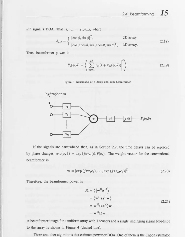
2.4 Beamforming
The purpose of array processing is to isolate a wanted signal from interfering signals
and noise and to estimate parameters of the isolated signal such as DOA or power. This is
spatial filtering. A beamfonner (also known as delay-and-sum beamfonner and conventional
beamfonner) estimates received power, Pb( ¢, 8), as a function of DOA [Pil89]. It delays the
hydrophone signals and sums them so that, for a given look direction, a signal arriving from
that direction is summed coherently (see Figure 3). The summed signal is squared and averaged
to obtain a power estimate. Signals not in the look direction are summed destructively. The
2.4 Beamforming
15
nth signal's DOA. That is, Tm = Xm84>,B, where
{
[coscp,sincp]T,
84> B =
, [cos
cp
cos (), sincp
cos () , sin ()]T ,Thus, beamformer power is
2D array
3D array.
Pb( </>,0) = \
fl
zm(t
+
T m (</>,0)) ) .Figure 3 Schematic of a delay and sum beamformer.
hydrophones
{
1_ Pb(<I>,8)
(2.18)
(2.19)
If the signals are narrowband then, as in Section 2.2, the time delays can be replaced
by phase changes, wm(</J, ()) = exp (j7rTm(</J, 8)cs). The weight vector for the conventional
beamformer is
w = [exp (j7rTIC s), ... , exp (j7rTMCs)]T.
Therefore, the beamformer power is
Pb =
(IWHZI2)
=
(WHZZHW)
=
WH(ZZH)W
-
HR
- w w.
(2.20)
(2.21)
A beamformer image for a uniform array with 7 sensors and a single impinging signal broadside
to the array is shown in Figure 4 ( dashed line).
There are other algorithms that estimate power or DOA. One of them is the Capon estimator
which I will describe without going into any mathematical detail. The Capon estimator has
better resolution than the conventional beamformer but it is more sensitive to sensor-position
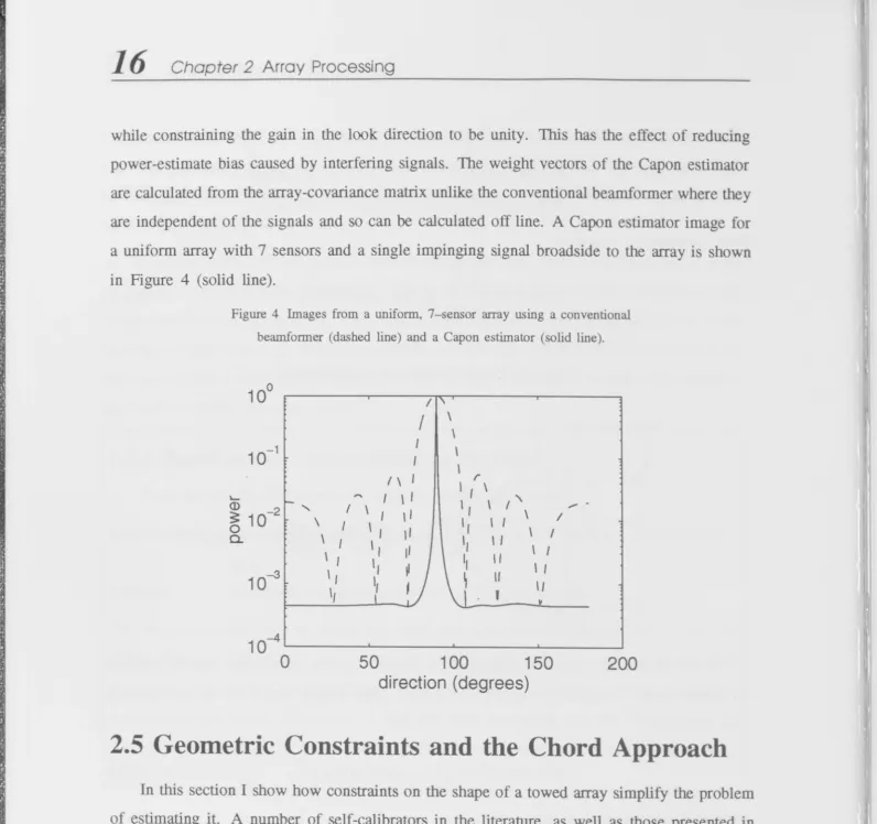
[image:30.809.34.788.23.990.2]16
Chapter 2 Array Processingwhile constraining the gain in the look direction to be unity. This has the effect of reducing
power-estimate bias caused by interfering signals. The weight vectors of the Capon estimator
are calculated from the array-covariance matrix unlike the conventional beamformer where they
are independent of the signals and so can be calculated off line. A Capon estimator image for
a uniform array with 7 sensors and a single impinging signal broadside to the array is shown
in Figure 4 (solid line).
Figure 4 Images from a uniform, 7-sensor array using a conventional
beamformer (dashed line) and a Capon estimator (solid line).
10° I
/
\ \1 0-1
~
\1 \ / I r
~
10-
2r "\
" I \ I I I \ I "\
I \ / \
,
\,
\ '"-\ I
I \
,
'I \ I,I \ I
Q. \
'I ,I " \ / \ I I
'I " \ I
1 0-3
~
\ I I, ~,
~ \I \ I II\/ I \ I - ~
10-4,
0----'---50 100 150 200
direction (degrees)
2.5 Geometric Constraints and the Chord Approach
In this section I show how constraints on the shape of a towed array simplify the problem
of estimating it. A number of self-calibrators in the literature, as well as those presented in
Chapter 4, make use of what Gray et al. [GWR89] call the chord approach. The chord
approach is simply a method of combining known constraints on the array's geometry with a
calibrating signal's phase- or time-delay information to estimate the array shape. It is assumed
that the array is 2D and the calibrating-signal source lies in the plane of the array.
Self calibrators can give estimates of the shape of an array and the DOA of the impinging
signals in relation to the estimated shape. However, there will always be a rotational and
reflectional ambiguity to the shape unless supplemental information is available!. In this section,
I show how a single heading sensor added to the array can eliminate the rotational ambiguity and
[image:31.827.5.801.21.768.2]2.5 Geometric Constraints and the Chord Approach
17
a second heading sensor can eliminate the reflectional ambiguity. The supplemental
heading-sensor information is easily integrated with the chord approach.
Let the inter-hydrophone arc length of the flexible cylinder bearing the array be p. If the
flexible cylinder is assumed not to stretch then each hydrophone must lie within a circle (or
sphere in 3D) of radius p that is centred on the previous hydrophone. Further, if the distance
between hydrophones is not large then the flexible cylinder can be approximated by straight
line segments between hydrophones. Each hydrophone will, therefore, lie on the circumference
of the circle (or sphere in 3D) of radius p that is centred on the previous hydrophone (see
Figure 5). That is,
(X m - xm_I)2
+
(Ym - Ym_l)2 = p2. (2.22)Figure 5 Model of the segmented array approximation.
fleTle
CY~der
-The distance between the wavefronts of the calibrating signal arriving at one hydrophone
and the next, dmn - dm-1,n, equals the difference between the relative arrival times of the
signal multiplied by the speed of sound,
dmn - dm-1,n = cs(tmn - tm-l,n)' (2.23)
I will drop the subscript n because we are dealing with only one signal. Assume that the
DOA of the calibrating signal, <p, is known. A coordinate system is chosen so that the first
hydrophone is at the origin and the tow vessel is travelling in the negative x-direction. To be
consistent with the relative time of arrival, tm, the location, (xm' Ym), of the m th hydrophone
must be on the straight line
(x m - Xm-l) cos <p
+
(Ym - Ym-l) sin 4> = dm - dm- 1.
(2.24)
This line is the signal's wavefront at a distance dm - dm - 1 before the (m - 1) th hydrophone. The
18
Chapter 2 Array Processingsimultaneous solutions to (2.24) and (2.22) so to resolve this twin ambiguity we choose the
solution that is closest to the tow-vessel's path (i.e. the x-axis), given by
m
xm = cos ¢(dm - d1 )
+
sin ¢L
Vp2 -
(dk - dk _ 1)2
k=1
m
Ym
=
sin¢(dm - d1 ) - cos ¢L
Vp2 -
(dk - dk_r)2,
k=1
and as shown in Figure 6.
Figure 6 Choose the solution closest to the tow-vessel's path.
hydrophones
~
<::J--o
Xm-l
Direction of ship's motion
Figure 7 Estimating signal direction using two hydrophone pairs with heading sensors.
4····.
dj-l - d/
::
' f
Xj-l
r ... I ... I
~""""""'p
....
\
...
~hydrophone
~
--- ---
X
- - - - k-l
<Pk
compass
(2.25)
When the calibrating signal's DOA is not known it must be estimated. It can be seen from
Figure 7 that dj - dj- 1
=
P cos ¢j, and so¢j
=
cos-1 (cs(tj - tj-l)/p)
(2.26)which has two solutions. We resolve this ambiguity by equipping two pairs of adjacent
hydrophones, (j -1,j ) and (k -1,k), with heading sensors to measure the absolute bearing
of their baselines. Each pair of hydrophones will give two solutions, one corresponding to the
real source direction,
9
]
,
and the other a virtual source direction, ¢J.
The virtual source always2.5 Geometric Constraints and the Chord Approach
19
source whether it be real or virtual is aj
=
<Pj+
f3j where f3j is the heading sensor measurement of that baseline. If f3j=I
13k
then aj=
ak
and aJ=I
at.,
which eliminates the ambiguity. Iff3j
=
13k
the two special baselines are parallel and the ambiguity can not be resolved.Chapter 3 Inverting the Spatial
Correlation Function
3.1 Problem Description and Background
In the literature on towed-array self calibration there is an implicit assumption that there is
enough information in the impinging signals to estimate both the array shape and the signals'
parameters. It is important to verify that this assumption is true; and under what conditions.
The conditions tell us whether there are certain assumptions that a self calibrator must make
to estimate the array shape unambiguously and, if the assumptions are incorrect, what form an
ambiguity will take. The form of an ambiguity might be whether a sensor exists in one of a
finite number of positions or in one an infinite number. This chapter deals with both generic
and towed arrays. I show that for towed arrays, if there is only one signal, every hydrophone
will have two possible positions. If there is a second signal the ambiguity is eliminated.
I present the necessary conditions for uniqueness of the spatial correlation function's inverse.
That is, I give the conditions for the locations of an array's sensors and the parameters of the
signals that impinge upon the array to be unique. The only information used is the exact
narrowband array-covariance matrix which is derived purely from the impinging signals. No
attempt is made to analyse the sensitivities of the sensor and signal parameters' estimates when
the array-covariance matrix is not known exactly. Nor does this chapter include algorithms for
estimating these parameters, only evidence that a hypothetical algorithm will or will not have
a unique solution to search for. In the manner of control systems theorists, I will say that the
sensor and signal parameters are observable if they are unique for a given array-covariance
matrix.
If the signals are incoherent with each other then at least three signals for a two-dimensional
array, and six for a three-dimensional array are required to determine the sensor, signal and noise
parameters uniquely. If all signals originate from one source, and are thus coherent with each
other, there is an infinite number of solutions for the sensor and signal parameters. The question
of observability is unanswered when there are coherent signals and two or more signal sources.
Observability of the sensor and signal parameters was investigated by Rockah and
Schultheiss [RS87a, RS87b], for two-dimensional arrays. They assumed that the signals are
3. 7 Problem Description and Background
21
is useful if one has the option to deploy controlled signal sources, or can otherwise guarantee
that the signals will be disjoint Rockah and Schultheiss gave the number of signals and sensors
required for observability, for both near- and far-field signal sources. They demonstrated that,
without additional information, translational or rotational uncertainties of the array shape and
signal field would be inevitable. Signals can only give information about the shape of an array
and the distribution of the signal sources in relation to the array; they give no information about
the absolute position of the array or its orientation. Thus, if one solution can be found for the
array shape and signal DOAs, any translation, rotation or reflection of that solution will also be
a solution (see Figure 8). These ambiguities can be eliminated by assuming that the location of
three sensors, two sensors and a signal DOA, or one sensor and two signal DOAs are known
a priori. However, for this chapter, I will regard all translations, rotations and reflections as trivial duplications of the one solution.
Figure 8 Translations (b), rotations (c) and reflections (d) are regarded as trivial duplications of the one solution (a).
:---I
---i---I ( ) , -
-: ; a
!
/
!
~)
---
r:;--:
I I
: : y .
:~ :I~
00""-__ • x ---. r ---.
I
I I I I
o
L. _____ • X~---~---~
: / A Y :
·
\
o~
Y
o
--.
x (c) (d)\~
' _ _ _ _ _ _ - - - _ . _ - - - _ _ _ _ _ _ 1
Lo and Marple [Lo92] investigated the more general problem of observability conditions
when the signals are not spectrally or temporally disjoint. TItis involved another question; are
the two or more steering vectors that make up the array-covariance matrix unique? Schmidt
[Sch81] called this rank-n ambiguity. Lo and Marple assumed that all the signals are incoherent
with one another, and that the noise-covariance matrix is known. They gave a proof for the
minimum required numbers of signals and sensors to estimate their parameters from the steering
vectors, which confirmed the results of [RS87a, RS87b]. The proof bears no obvious relation
to what is a geometric problem, and so is not illuminating.
Here I discuss the following topics that are not treated in [RS87a, RS87b, Lo92]:
observ-ability of the noise-covariance matrix, 3D arrays, coherent signals and closed-form solutions