An experimental study of particle sizing in static condition and in shear flow by diffusing-wave spectroscopy

(1)

An Experimental Study of Particle Sizing in Static

Condition and in Shear Flow by Diffusing-wave

Spectroscopy

Thesis submitted in accordance with the requirements of the

University of Liverpool for the degree of Doctor in Philosophy

by

Huan Huang (BEng, MRes)

(2)

I

Abstract

This thesis focuses on the micro/nanoparticle size measurement by using Diffusing-wave Spectroscopy, investigating the laser power and concentration effect on the measurement and researching the measuring method for particles in shear flow. A DWS-CCD backscattering experiment set-up was used in this project. By using this set-up, in all about 2000 experiments were performed during the project, including system testing, laser power influence study, concentration effect study and shear flow study.

In the beginning, a detailed analysis of the particle sizing for particles in static condition was carried out by summarising the principles and procedures. The results revealed that the experimental set-up in this work was reliable and repeatable. A calibration process was still required for the CCD’s frame rate and resolution, the light absorption and the CCD’s position in the set-up. After determining some important parameters, the research was extended to laser power and concentration influence study. The autocorrelation functions were produced under different laser power and for different concentration of particle solution. Analysis confirmed the influences, and the results were expressed in formulas to describe specific effects for laser power and solution concentration. Based on the formulas, new equations









2 2 2 2 0 1 1.83 16 1 2.5 B

n K T

R S         

 and





2 2 0.531

2 2 0

224

1 2.5 B

n K T

R

S

  

  

 

 for particle sizing were

derived for different concentration ranges. After that, particle’s motion and light scattering in shear flow were investigated. It was concluded that three regions could be used to describe the particle’s movement under shear force; in different regions, the autocorrelation functions were different due to the variation of the characteristic time scales. The Brownian motion and shear strain dominated particle’s movement under specific flow velocities. Therefore, for particles subjected to high flow velocities, a new particle sizing formula

1 6 _{1 3}

2 3 ₂ 0

2

3 1

1

64 5 N 1 cos

k m R n m S        _  _ _ _ _ _   _ _ _ _        

  was produced to distinguish the general

formula which was only valid for particles under Brownian motion.

(3)

II

(4)

III

Acknowledgement

First of all, I would like to thank the University of Liverpool and the ORSAS committee for funding my PhD study in these years.

Second, I want to express my deep gratitude to my supervisor, Professor Doayi Chen and Dr Xiaoxian Zhang. They have offered me the opportunity to study here and gave me valuable guidelines and advice during the research. I am very lucky to have Dr Zhang as my supervisor in the final year who spent a lot of time on reading my thesis and gave me comments and suggestions.

I am also grateful to my colleagues and all of the staff in Civil Engineering, for their selfless help and support through my study in Liverpool.

I sincerely thank Mrs Denise Bain whom I always request help from. Most of the material I used in my experiment was ordered by her. I am also thankful to the technicians in School of Engineering, Mr Martin Jones, Mr Derek Neary and Mr Clive Whittam. They made some of the experimental apparatus and helped me on my laboratory work.

(5)

IV

Publications

1, D. Y. Chen and H. Huang, Interaction of Flows and Particles at Sub-micrometer Scales,

Environmental Fluid Mechanics Memorial Volume in honour of Professor Gerhard H. Jirka , Karlsruhe, Germany. June 2011.

(6)

V

List of Figures

Figure 2.1 Statistical diameters used for irregular particle size characterization. ... 10

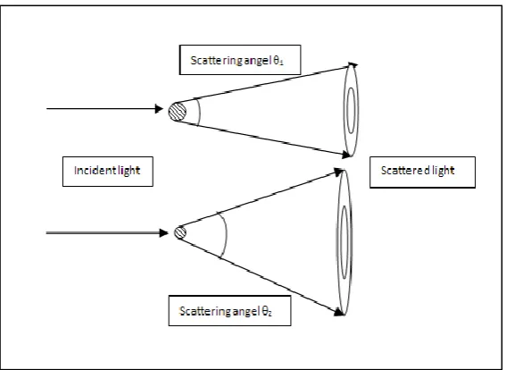
Figure 2.2 Diagrammatic description of light diffraction denoting that the particle size information is contained in the scattered light signal. ... 13

Figure 2.3 A classic DLS experiment setup... 15

Figure 2.4 The scattering geometries for normal one-beam light scattering (a), two-colour DLS (b) and three-dimensional DLS (c). ... 17

Figure 2.5 Photon enters the sample slab and executes random walk until leaving the slab. .. 21

Figure 3.1 The diagram of Experimental set-up and arrangement for DLS (a) and DWS (b). 26 Figure 3.2 Diffusing-wave spectroscopy set-up which works for both transmission and back-scattering geometries[37]. ... 27

Figure 3.3 The schematic representation for DWS experimental set-up, transmission geometry(a) and backscattering geometry(b). ... 28

Figure 3.4 H8711 multianode photomultiplier tube made by Hamamatsu[93]. ... 30

Figure 3.5 Fastcam Ultima APX CCD system made by Photron[96]. ... 31

Figure 3.6 The DWS experimental set-up in this project. ... 32

Figure 3.7 the Argon Ion laser applied in the experiment as a light source. ... 33

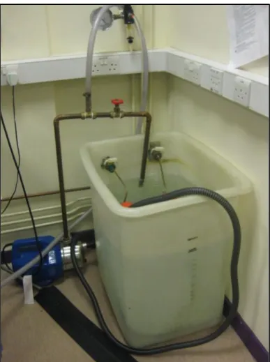
Figure 3.8 The water was stored in a tank and then pumped into the cooling system. ... 34

Figure 3.9 Two lenses with a distance of 60mm between each other were used to expand the laser beam. ... 35

Figure 3.10 A part of the CCD system: APX processor and PC installed with synchronizing software. ... 36

(10)

IX

Figure 3.12 Sample cell made of microscope slides with a 1x1x75mm3 channel. ... 38 Figure 3.13 Sample cells made of plastic square-tubes with channel dimension: 3x3x180mm3, 3x6x180mm3 and 6x6x180mm3, respectively. ... 38 Figure 3.14 Suspension in syringe was injected into sample cell by syringe pump, and finally discharged into reservoir. ... 39 Figure 3.15 2ml 500nm latex beads solution with 10% with weight purchased from Sigma-Aldrich. ... 40 Figure 3.16 15ml 3200nm latex beads solution with 1% with weight purchased from Duke Scientific. ... 40 Figure 3.17 300nm latex suspensions with different concentrations: 1%, 0.1%, 0.01% and 0.001% (from left to right). ... 41

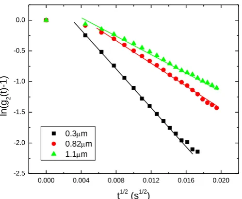
Figure 4.1 The image of particles with diameter of 1100nm under microscope with total 200x magnification. ... 45 Figure 4.2 The image of particles with diameter of 300nm under microscope with total 200x magnification. ... 45 Figure 4.3 A snapshot of 1100nm-diameter particle under CCD monitoring. This picture is a frame image captured from a video in which the particles were in Brownian motion. ... 45 Figure 4.4 A frame of particle images taken by APX CCD camera. ... 47 Figure 4.5 Autocorrelation functions for 300nm-, 820nm- and 1100nm-diameter polystyrene particles in 1.8% (volume fraction) solution, respectively. ... 51 Figure 4.6 Intensity autocorrelation from a typical DWS measurement in backscattering geometry. Plotting lg_g₂

 

t 1_vs t , shows linear decays over a broad range of decay

(11)

X

Figure 4.7 The autocorrelation functions g t₂

 

1of different pixels resolutions are showed

for the 820nm-diameter particle sample with 1% concentration (in weight). ... 54

Figure 4.8 Comparison of results of different “effective” absorption lengths la, no absorption with the experiment results of the autocorrelation functions for 820nm-diameter particle in 1.8% volume fraction. ... 56

Figure 4.9 The CCD was placed at various locations to work out different values of γ. ... 57

Figure 4.10 The contour plotting of γ. ... 58

Figure 4.11 3D view of the contour plotting of γ. ... 58

Figure 5.1 DWS autocorrelation functions G t₂

 

for the 300nm latexes particle at 1.8% volume fractions with laser powers ranged from 40mW to 1440mW: a) laser power at or above 640mW is sufficient for DWS and all curves from 640mW to 1440mW claps together; b) a large variation displayed for the laser power range between 40mW and 320mW. ... 64

Figure 5.2 Normalisation of DWS autocorrelation functions g₂

 

t for the 300nm latexes particle at 1.8% volume fractions with laser powers ranged from 40mW to 320mW: a) normalised for g₂

 

t to cover the full range between 0 and 1; b). logarithm plotting against t1/2 shows a linear decay over a broad range of decay times. ... 66

Figure 5.3 Compare the normalised g₂

 

t of 1.8% volume fraction 300nm suspension in the low laser power band (40mW to 320mW) and high laser power band (640mW to 1440mW): a) plotting g₂

 

t against time t; b) log plotting against t1 2 show more than 30% difference in the slopes... 67

(12)

XI

Figure 5.5 Compare the normalised g₂

 

t of 0.9% and 9% volume fraction for 300nm suspension in the low laser power band (40mW to 320mW) and high laser power band (640mW to 1440mW), plotting g₂

 

t against time t. ... 69 Figure 5.6 Compare the normalised g₂

 

t of 0.9% and 9% volume fraction for 300nm suspension in the low laser power band (40mW to 320mW) and high laser power band (640mW to 1440mW), log plotting against t1 2 show more than 58% and more than 15% difference in the slopes, respectively. ... 70 Figure 5.7 Slopes of DWS autocorrelation functions ln_g₂

 

t _ against t1 2 for the 300nm

latexes particle from 0.9% to 9% volume fraction (1% to 10% concentration by weight) and laser powers of high band, low band and 320mW respectively. ... 71

Figure 6.1 When the concentration is a constant, the decay rate of g₂

 

t deceased with particle size increase. ... 80 Figure 6.2 the decay times of the autocorrelation functions as a function of particle diameter at volume fraction 0.9%, 0.18%,0.36%, 0.54%, 0.72% and 0.9% (1%, 2%, 4%, 6%, 8% and 10% in weight). ... 81 Figure 6.3 DWS autocorrelation functions for the 300nm latexes particle with volume fractions from 0.09% to 9% (0.1% to 10% concentration by weight): a) auto correlation functions g₂

 

t ; b) normalised g₂

 

t to cover the full range between 0 and 1. ... 82 Figure 6.4 Variation of slope S in the range of 0.09% to 9% volume fractions (0.1% to 10% concentration by weight) in a 1 by 1mm channel: a) the effects of concentration on S are in line with previous theory; b). A function is used to describe the variations. ... 85 Figure 6.5 DWS autocorrelation functions normalised g2(t) for 300nm latexes particle with

(13)

XII

Figure 6.6 DWS autocorrelation functions normalised g2(t) for 300nm particle with

concentration from 0.0001% to 0.01%. ... 88

Figure 7.1 Pictures of Polystyrene particles taken in sequence under the image field of microscope . ... 91

Figure 7.2 The auto-correlation functions for different particle solutions in 3x3 mm sample channel under various shear flows. The legends denote series of flow rates. ... 99

Figure 7.3 The autocorrelation functions (a) and logarithm plotting against time square (b) for 1% 500nm particles in a 3x6mm sample channel under shear strain. ... 100

Figure 7.4 the plotting of slope against flow velocity for (a) 100nm-, (b) 300nm-, (c) 500nm-, (d) 820nm- and (e) 3200nm- diameter particles tests in 3x3mm2 sample cells. ... 103

Figure 7.5 The graph shows the low and high boundary between Brownian and shear flow effects. ... 104

Figure 7.6 The three regions, Brownian motion dominant area A, transition area B and shear flow dominant area C. ... 105

Figure 8.1 The principle of turbidity measurement. ... 115

Figure 8.2 The spiral channel designed for future experiment. ... 118

Figure 8.3 The PMT-ADC system for future work. ... 118

(14)

XIII

List of Tables

Table 4.1 The values of  are determined from the slopes and other parameters for 300nm, 500nm, 820nm and 1100nm latex samples respectively with 1.8% volume fraction... 52 Table 4.2 The particle sizing for 300nm, 500nm, 820nm and 1100nm latex beads samples respectively with various volume fractions, when  2is specified. ... 53

Table 6.1 The particle sizing results for concentrated solution with a volume fraction range of 0.9% - 9%... 86 Table 6.2 The particle sizing results for concentrated solution with a volume fraction range of 0.09% - 0.9%... 86

(15)

XIV

List of Abbreviations and Symbols

Abbreviations

CCD Charge-coupled device

CHDF capillary hydrodynamic fractionation DLS dynamic light scattering

DWS diffusing-wave spectroscopy

EPSRC Engineering and Physical Sciences Research Council NTU Nephelometric Turbidity Units

PIV Particle image velocimetry PMT photomultiplier

PS Polystyrene

TEM transmission electron microscope TiO2 Titanium Dioxide

Symbols

Greek Letters

 Decay time s

0

 The characteristic diffusion time s

 The ratio of a circle's circumference to its diameter -

 _{Diffusion constant} _-

 Scattering angel Degree

 The total scattering cross-section m2

 Wavelength of light m

 The coherence factor -

 Volume fraction -

0

 Viscosity of water Pa·s

s

 Viscosity of the solution Pa·s

B

 The characteristic time scale representing Brownian motion s

S

 The shear relaxation time s

 _{Fluid density} _kg/m3

 _{Dynamic viscosity of the fluid} _kg/m·_s

 Speed of light m/s

 Shear rate s-1

N

(16)

XV

Latin Letters

a Width of the cross-section of the flow cell m

b Depth of the cross-section of the sample cell m

0

D The diffusion coefficient of spherical particles m2/s

eff

D The effective diffusion coefficient m2/s

d Particle’s diameter m

E The total scattered field lm·s

0

E The scattered field received by the detector lm·s

 

1

G t The electric field autocorrelation function -

 

2

G t The light intensity autocorrelation function -

 

1

g t The normalized electric field autocorrelation function -

 

2

g t The normalized intensity autocorrelation function -

 

H q The function to express the effect of the hydrodynamic

interactions -

I The scattered light intensity cd

P

I The light intensity of pth pixel cd

out

J The flux of photon lm

B

K Boltzmann constant J/K

0

k The wave number -

l The scattering mean free path m

a

l The absorption length of the medium m

*

l The transport mean free path m

L Thickness of sample cell mm

m The ratio of the refractive index of the particle to that of the

medium -

n The refractive index -

e

P Peclet number -

 

P s the distribution of photon path of length s -

q _{Wave factor} -

Q The flow rate ml/m

R Particle radius m

e

R Reynolds number -

i

r Position of the ith particle -

in

r The light incident point on sample cell -

out

r The light escaping point from sample cell -

 

2

r 

(17)

XVI

s Photon’s path length m

S The slope of autocorrelation function logarithm plotting against

time square -

 

S q The static-structure factor -

T The absolute temperature K

t Time s

U energy density of light lm·s/m3

max

V The maximum velocity in the centre of the flow channel m/s

 

X t The average contribution of a scatter to the dephasing of a light

path -

0

(18)

1

Chapter 1 Introduction

1.1 Background

Nanotechnology is the scientific research which has been developed recently, however, it has been intensively involved in human’s life nowadays. It is a rapidly evolving area with knowledge related to study the matters at the molecular level, and it is purposeful of controlling, manipulating or handling these particles at these very small scales[1].

A particle is a small subject that has a specific dimension in geometry and has uniform properties as a unit. Particles can be classified according to their sizes. Generally, particle with a diameter of 1-1000 micrometer are categorized as microparticle; 0.1-1 micrometer as sub-microparticle. If the diameter is in the range from 1 to 100 nanometer, the particle is grouped in the category of nanoparticle. This is one classification that has been accepted by most scientists and researchers[2-4].

Particles with diameter ranging from 1 nanometer to 1000 micrometer are frequently encountered in industries and in our domestic life. They could be in the forms of solid, solution, foam, aerosol, gel or colloid. They exist extensively in a wide range of materials, such as latex, polymer, ceramic, metal and carbon, and have important applications in biology, chemistry, physics and medicine. The particles in micro- and nano-scale have such a significant application in science and technology, and hence they have been widely regarded as one of the most important scientific discoveries of modern science.

(19)

2

was also performed in Japan from 1980 to 1986. It was a nanoparticle project reported by Hayashi et al.[6]. In the1990s, “ultrafine particles”, was replaced by the new name “nanoparticle”, and since then nanoparticle has been a widely accepted name by most researchers[7].

Compared to large particles, nanoparticles have significantly different features, dependent on their size. They are different from the bulk material which is made up of small objects[8]. They are an effective bridge between bulk material and molecular structures, and display various characteristics in optical, electrical, magnetic and thermal properties[9]. Most unique properties of micro/nanoparticle are due to their increased surface area and the altered surface structure, making them more active in certain circumstance. For example, the high surface-area-to-volume ratio of micro/nanoparticles leads to a high absorption and diffusion. Due to these features, Titanium Dioxide nanoparticle works as an effective photo-catalyst[10], and Zinc Dioxide performs excellently to block UV radiation[11]. Furthermore, these features provide advantages which are shown as stiffness, resistance and reinforcement for some material. For instance, ceramic made up of nanocomposites and nanocrystalline has high level of tenacity, and is corrosion-resistant; the mechanical properties have been dramatically enhanced[12].

Over the past 20 years, the research of micro/nanoparticles has made great progress, and a new technology, nanotechnology, has been developed.

(20)

3

Nanotechnology has a wide application in biology, medical science, physics, chemistry and engineering. For example, to avoid food spoiling or decaying in food packaging, one can add silicate nanoparticles to plastic film to prevent gasses (such as oxygen) or moisture entering the package[16]; and in coating industry, zinc oxide nanoparticles can be sprayed on cotton surface to block up UV irritation, for anti-bacteria purpose[17]; in textile industry, silver nanoparticles can be embedded in the fabric to kill bacteria to keep cloth fresh[18]. In biomedicine, protein carrying medicine can be coated with iron oxide nanoparticles, and these particles are then injected into blood vessel and travel with blood cells. When they reach the lesion position, the medicine is released directly and rapidly to the target. This can reduce the side effects of the medicine on patient’s organs in blood circulation system (such as liver, kidney and spleen) and increase the bioavailability of drugs in comparison with other traditional delivery methods[19].

Nanotechnology has also been applied in environmental engineering to eliminate the toxic and hazardous substances in water and air[20]. For example, using titanium dioxide as a photo-catalyst is one of the most promising methods to deal with refractory organic contaminants in water and wastewater[21], in which titanium dioxide, in powder with nano-scale particles, is released to the contaminated water. When it absorbs UV radiation from sunlight or illuminated light source, the electron will be stimulated, creating the negative-electron and positive-hole pair that has strong oxidizability. Under oxidation, most organic pollutants and inorganic pollutants can be decomposed to water and carbon dioxide[22]. Since catalysts do not involve in the chemical and biochemical reactions, the nanoparticles are not consumed. Increased researches have proved that photo-catalysis works well with hydrocarbons, aromatic compounds, dyes, surfactants, pesticides, petroleum and cyanides, and during decolorization and detoxication, pollutants are mineralized to inorganic molecules[23, 24].

(21)

4

Commonly, they need post-treatment for recycle purpose, such as filtration, centrifugation and flocculation[26]. In these procedures, the particle size is a key element which influence and control the operation.

1.2 The Size of Micro/nanoparticle

Particle size is a key parameter of micro/nanoparticles that determines the particular properties of the bulk material. Tremendous research on particle dimension, size distribution and their dynamic properties in flowing water has been done in various fields, including food industry, chemical industry, pharmaceutical industry[27, 28]. For example, in producing drugs in solid or suspension forms, especially insoluble drugs, the particle size and size distribution could considerably influence the bioavailability of the medicine[29]. As a result, the measuring of particle size and size distribution is compulsory in medicine pulverization. Polymer synthesis, including emulsion and dispersion process, is also particle-size sensitive, especially when preparing polymer latexes[30]. In colloid chemistry, particles encounter weakly aggregation, therefore understanding the flow behaviour of particles is important[31].

In environmental engineering, the study of particle size is often required in the research of suspended solid sedimentation, turbidity measurement, contaminants degradation [32-34]. In coastal zone, the suspended matters are mixture of multiple particles, and they aggregate and break up under flocculation and erosion. The particle size is one index that reveals the dynamics of aggregation and sedimentation [35]. In research of photo-catalysis in recent 20 years, numerous issues have been addressed[20], including problems in fundamental study of photo-catalysis and photo-catalytic reactor, and in investigations of the characteristics and activities of catalyst particles in solution. For contaminants degradation, Tratnyek et al.[36] showed that particle size had effect on intrinsic activity of Fe0 particles, thereby influenced the kinetics of contaminant degradation. When using TiO2 as catalyst, Andronic et al.[37]

found that the particle size changes due to crystallization of TiO2.

(22)

5

advantages of light to detect the dynamic properties. It measures the time autocorrelation of light signal which is multiply scattered in a turbid medium and then obtain the particle size information[41]. Apparently, most DWS studies have used a fixed light power to illuminate the solution and obtained the scattered light signal to measure the particle size in suspensions with various concentrations. The process of particle sizing is affected by different laser powers and solution concentrations. First suggested by Chiu and Zare[42], biased diffusion and optical trapping forces lead to power dependence of particle sizing process. Kuyper et al. agreed that and confirmed the dependence in their research[43]. Navabpour et al. have reported the influence of concentration on particle sizing analysis[44]. Schefflod also said that in the past his research has been restricted in sufficiently dilute solution in which particle’s motion was predominate by Brownian motion. Actually at higher densities, the deviations of the measured correlation exist therefore the determination of particle size becomes more difficult[40]. Previous research proved that DWS is a reliable for multiple scattering systems when the system is sufficient dilute. However, the studies on the impact of laser power and particle concentration are rare.

Furthermore, due to the nature of DWS, most of the researches were carried out in stagnant mediums in which the particles only execute Brownian motion. Theoretical studies have showed the influence of Brownian motion and shear flow on the measured correlation functions, but experimental studies in dynamic systems, especially in laminar shear flow, which is more practical, is lack. In fact, one potential application of DWS in flow medium is for performing noninvasive measurement of the flow velocity. For example, Wu et al presented a technique using DWS in strongly multiple scattering medium for measuring velocity gradients for laminar shear flow[45]. Skipetrove et al. set up a model DWS experiment to study the particles in a flow of aqueous suspension which had similar parameters to some types of biological tissues; they believed that the technique had the potential for application in medical diagnostics, and their results had a extremely important impact on medical instrumentation[46].

(23)

6

1.3 Research objectives

The objectives of this research are to study the measurement of micro/nanoparticle size in multiple scattering systems, to investigate the laser power influence on the process of particle sizing and research the measurement accuracy for concentrated suspension. This study aims to gain a visible insight of DWS methods to understand the light effect, suspension concentration effect. Considering my background is environmental engineering, apart from concentrated suspensions, particle sizing is also investigated in very low concentration suspension. This study will help other researchers to develop a new device based on turbidimeter which not only provides readings of solution turbidity and also provides the size values of suspended particles.

In addition, experimental studies are also expanded to particle sizing in laminar shear flow. This study aims to quantitatively develop the relationship between the measured correlation functions and the flow velocities, to investigate the interaction between particles under the influence of Brownian motion and shear flow. Under the effect of Brownian motion and/or shear flow, the autocorrelation functions have different decay modes which result in different particle sizing formulas. Therefore, by knowing the onset of effect, the knowledge of particles dynamic properties in flow medium will be obtained, and corresponding size measurement can be carried out.

Overall, the research aims to provide some theoretical support to the instrumentation of particle size analysis, to help technicians to develop the on-line or in situ equipment for flow velocity and particle’s dynamic properties detection.

1.4 The Approach

(24)

7

The approach is presented in details as following:

 In the beginning, literature reading was carried out to gain an insight of methodology of particle sizing by DLS and DWS.

 In order to obtain the direct impression of micro/nanoparticles, the particle observation was taken place under optical microscope.

 Preparing for the experimental, the high CCD system was rent from EPSRC instrument pool, and the latex beads suspensions were ordered from Sigma-Aldrich and Duke Scientific.

 A back scattering CCD-DWS experiment was set up in laboratory. An Argon Ion laser was employed as light source. A high speed CCD camera was applied to capture particle images. The particle suspensions were prepared, and the sample cells with observing windows were manufactured.

 The experiment set-up was verified and calibrated by standard latex particle solutions. The boundary conditions were defined, including resolution and frame rates of CCD camera, light absorption and CCD’s position.

 In static status, the laser power tests and concentration tests were performed by setting various conditions (laser power outputs and volume fractions) according the research plan. Also, the experiments of particle sizing by DWS in very low concentration suspension were completed. Data was derived and collected. Processing and analysis were carried on in the same time with experiments.

 Experiments were performed in laminar shear flow. A large number of flow tests under different flow velocities in different sample cells were undertaken in the same experiment set-up. Data was continuously generated and collected from the lab. Properly processing was done, as well as analysis.

 The analysis was continued after the experiments. By assistant of some useful software, such as C++ programme, Matlab, Excel, Origin, the final results were produced and precisely presented in the form of table, graphs and texts. The results were presented in conference, and papers were submitted to journals.

1.5 Outline of the Thesis

This thesis includes eight chapters and the outline of each subsequent chapter is organized as follows:

(25)

8

 Chapter 2 gives the description of particle sizing methods. It elaborates the principle of DLS and DWS and presents the history and development of these methods. It also demonstrates the methodology of DWS in experimental research.

 Chapter 3 describes the DWS experimental set-up and the arrangement in Littlewoods Laboratory, including the installation of optical device, the material preparation and the operation of equipments. In addition, it discusses the issues about the equipment selections and experimental geometries.

 Chapter 4 presents the process of DWS method verification. Particle size measurement is also described in this chapter. Furthermore, it talks about the boundary conditions determination and calibration, including the camera’s frame rate and resolution, light absorption and the location of camera.

 Chapter 5 gives the summary of previous studies of laser power effect. Then it describes the laser power tests in this work. It reports the data analysis result of the tests. After that, discussion is made to present that the laser power may mislead particle sizing under a specific level. A conclusion is also given at the end of this chapter.

 Chapter 6 first summarizes previous work by other researchers, then gives the suspension concentration effect tests in this work. After the tests, results are presented to describe the influence in details. Also, two formulas are given for particle sizing under different concentration ranges. Apart from these, experiment has been performed on very low concentration suspension. In the final part, the same as Chapter 5, the experimental result discussion and conclusion are demonstrated.

 Chapter 7 is similar on structure to Chapter 5 and Chapter 6. It reports the experiment and results from flow tests which are conducted with flow fluid. The research studies the interaction between particles in flow and discusses the domination of Brownian motion or shear strain. The results are presented and a new formula is given for particle size measurement for particles controlled by shear force.

(26)

9

Chapter 2 Development of Particle Sizing Technology

2.1 Introduction

Measuring particle size is a great interest in many fields, including chemical industry, food industry, pharmaceutical industry, mining industry and environmental engineering. The particle sizing process is involved in any stage of the production. The properties of particles of particular materials are influenced by their shape, size, size distribution, surface area and stability[47, 48]. Hence, particle size is an important parameter indicating the quality of the material. For example, in pharmaceutical industry, the size of the particles of active ingredients is strictly managed to control the content uniformity[49], the dissolution rate[50] and the absorption rate of medicine[51]. In some procedures, such as milling and granulation that aim to reduce the particle size, the operation of size monitoring is required to obtain a desired particle size[52]. While, in crystallization, the particle size growth is also monitored during the process[53]. Measuring and controlling the particle size can help maintain the consistency of products, improve the quality of products, enhance the value of products and maximize the commercial profitability. Therefore, the measurement of particle size is a necessary procedure.

(27)

10

2.2 Particle Size Definition

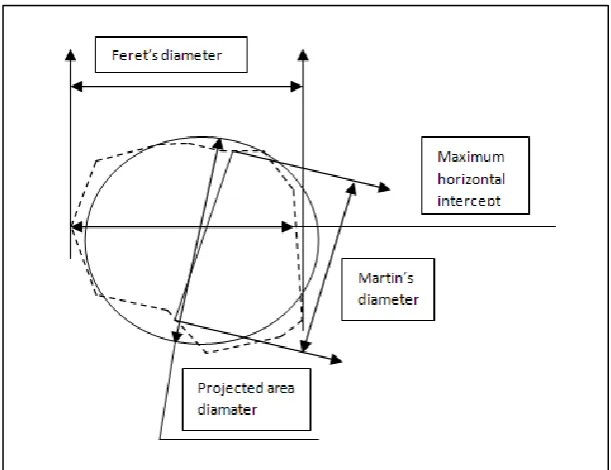
[image:27.595.145.451.367.602.2]

Particle size is a parameter that describes the dimension of the particle; the particle can be solid, liquid or gaseous. The shape of the particle varies. For spherical particle, the size characterization is simple. If the particle is non-spherical, the description of particle dimension might need several parameters: its length, breadth, thickness and description of the overall shape[58]. Besides, an imaginary sphere can also be used, replacing the real particle to get an equivalent dimension[59]. The imaginary sphere can be a sphere having the same volume, weight or surface area with the given particle. Hence, the equivalent dimension of a particle could be either weight-based size, volume-based size or area-based size. For irregular particles, the characterization of particle size must include the equivalent diameter and particle shape. The commonly used particle diameters are the Feret’s diameter, the Martin’s diameter, the projected area diameter, the maximum horizontal intercept[60]. As shown in Figure 2.1.

Figure 2.1Statistical diameters used for irregular particle size characterization.

(28)

11

measurement of particle size; however, Feret’s and Martin’s diameter are more practical to conduct with the assistant of an eyepiece scale or filar micrometer. They are widely used, but an average value over all possible orientations should be give to minimize variation due to the random orientation[61]. Besides, the maximum horizontal intercept which means the largest length of the horizontal intercept of the particle profile also should be determined as an average value over the orientations[60]. In practical application, a combination of methods is required to provide more precise quantity of the size[58].

In fact, the diameter mentioned above is the average particle size for particles defined by particle sizing methods which are based on microscopy images. There are other methods which provide some different definition. For example, the volume equivalent particle size, the hydrodynamic particle size. The hydrodynamic particle size is often employed to describe the radius of a hypothetical hard sphere that has the same diffusion coefficient as the particle under examination; it is derived from the Stokes-Einstein equation by using light diffusing measurement[62]. It is easy to define the size of a single particle, but difficult for the ensemble of particles due to the diversity. Hence, the hydrodynamic particle size often is measured and employed to describe the mean average particle size which will be discussed in the following.

2.3 Particle Sizing Technology

When the particle size gets smaller into micrometer, determining its size becomes increasingly difficult. However, the problem has been sort out by the improved technology. A wide range of techniques are involved for accurately particle sizing research. Commonly, the optical microscopy, laser diffraction, digital image analysis and dynamic light scattering are used. When measuring the particle size, there is no method that suits all particle samples. The best way to obtain a good result is choosing a proper method according to the particle’s properties.

(29)

12

reading the stage micrometer and the ocular micrometer. Or, particle’s images are analyzed on the basis of coordinates, and the size is then estimated by counting the number of pixels[64]. This method is direct and simple for operation. However, it is an accurate way only if a representative enough number of particles are counted[30]. The minimum analysed particle number is the key point of this technique. According to Vigneau et al.[63], an average number of at least 1500 particles or more is suggested. Furthermore, the particles cannot be altered during the preparation of the mounting process. Therefore, the sample preparation is a job which needs time and patience. Besides, the resolution of the optical system highly controls the accuracy of the measurement[65]. All of these limit the extensive application of optical microscopy for size measurement. It is often regarded as a method just for calibration.

(30)

[image:30.595.157.441.70.277.2]

13

Figure 2.2 Diagrammatic description of light diffraction denoting that the particle size information is contained in the scattered light signal.

Particle image velocimetry (PIV) is a method based on the analysis of digital images of small seeding particles which is used to track flow[69]. In the beginning of the development, it was applied in velocity field measurement. Later, Chen et al.[70] used this digital image analysis method to study bubble size. In the work of Cheng et al.[71], it was developed to determine the geometrical properties of small particles. In their study, the particles suspension was illuminated by laser and strobe light to produce the light-scattering images and diffusive back-lighting images which were full of particle spots. These images were captured by high speed camera and processed by PC. In the picture, each particle spot occupied a particular projected area with a number of pixels. If the relationship between pixel and real length was known, then the particle size could be determined. Digital image analysis dose not withdraw particles from the media, no matter the sample is monodisperse or polydisperse; it is a solution with no intrusion. In addition, it can provide particle shape information, not only particle size. It is a simple and inexpensive method for particle dimension measurement [72]. Therefore, this method can be easily incorporated into basic aggregation modelling frame work[71]. It is always jointly used with laser diffraction to gain a deeper understanding of the particles.

(31)

14

Elizalde et al.[30], it is concluded that if only the average particle size is sought with no importance of the whole particle distribution, DLS might be the best option.

2.4 Dynamic Light Scattering

2.4.1 Classic Dynamic Light Scattering

Dynamic light scattering (DLS, also known as photo correlation spectroscopy or quasi-elastic light scattering) is a powerful light scattering technique in micro- and nano-technology. It is a well-established spectroscopic method for studying single-particle (for dilute solutions) and collective particles dynamics in a variety of systems[73], such as solution, gel, foam and aerosol. It can measure the hydrodynamic particle size in a wide range. The technique is based on the fact that laser beam passes through solution or colloidal system can result in scattering of light by suspension particles. The scattered light fluctuating with a characteristic time scale provides valuable information about the size of the particles in this system[74].

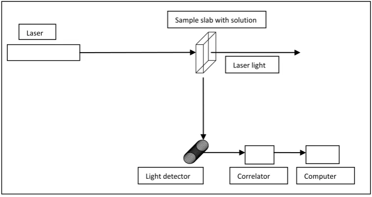
In the classic DLS experiment (see Figure 2.3), a dilute particle solution is illuminated by a laser beam. Then, the laser light is scattered by the particles. At the side face, a detector is set to collect the scattered light from the solution. The principle of DLS was as following[75]: first, particles have a particular set of position in the scattering volume. The different position and the different distance between particle and the detector result in different scattered waves; second, the light source has different incident phases when they approach particles positions. Therefore, the relative phases of scattered wavelets are diverse. At time t, the detector receives a electric field of E t

 

that is the superposition of all scattered wavelets. When time elapses to , the new slightly shifted electric filed yield due to Brownian motion of the particles is updated toE t







. Setting the autocorrelation function of the electric fieldg₁

 

 , the normalized form of the intensity autocorrelation function g₂

 

 can be expressed in a relationship withg₁

 

 . From the specific scattered light intensity autocorrelation function

 

2

(32)

15

calculation of its moments or cumulants. This method has statistical accuracy and can be incorporated with other data analysis.

DLS works in static and monodisperse system which means the absence of multiple scatterings. In this system, each photon has been assumed to be scattered by particle exactly once before it is detected. Therefore, DLS cannot provide an insight into particle’s dynamic properties in multiple scattering events. According to Zakharove et al.[78], in a high-order scattering system with a light transmission lower than 95%, a few things could be altered compared to low-order scattering system. First, the intensity autocorrelation function starts to decay quickly, which does not act as DLS theory. Second, due to the superposition of several scattering events, the scattering angel and wave number cannot be interpreted accurately. Therefore, DLS is limited in investigation of low particle concentration suspension, in which only single scatterings take place. For the multiple scattering medium existing in a variety of systems, in which particles produce strong scattered intensities, new technique has been developed based on DLS to meet the requirement of research and industry.

2.4.2 Improved Dynamic Light Scattering for Concentrated System

In order to solve the problem that DLS is unable to work in highly turbid system, the cross-correlation approach has been developed[79, 80]. This method has been validated by two simultaneous DLS experiments which are performed on the identical scattering volume to obtain the same cross-correlating signals, sharing the same scattering vector in different geometries and suppressing the multiple scattering [81]. The correlated intensity fluctuation

Laser

Sample slab with solution

Correlator

Light detector Computer

[image:32.595.108.487.133.333.2]

Laser light

(33)

16

on both detectors is generated only by single scattered light, while the uncorrelated fluctuations produced by multiple scattered light only contribute to the background[81]. The improved method has been proved to be successful and it has been reported in more versatile ways in the published papers presenting two-colour DLS and three-dimensional DLS[81, 82].

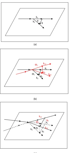
In the dual-colour cross-correlation experiment of Schatzel et al.[83], two colour coded beams were used, and two of the possible four paths were selected. In their design, the identical scattering volume and scattering vector were chosen for both colour. The light fluctuation was isolated due to a large range of scattering angles. The isolation played an important role in extracting static structure data. While, different from two-colour DLS in which the incident and scattered beams all lie in the same plane, in three-dimensional DLS, two incident beams with the same colour are slightly above and slightly below the scattering plane, and the detectors are correspondingly placed above and below the plane[84]. In the special geometry, the incident beam, which enters the sample above the plane, and the scattered beam, which is below the plane, build up a light path, defining the same scattering vector. Another path is generated similarly but inversely. Figure 2.4 shows the scattering geometries for normal single beam light scattering, dual-colour DLS and three-dimensional DLS, respectively. k₁ and k₁₂represent the incident light propagation vector. k₂and k₂₂

(34)

17 (a)

(b)

[image:34.595.153.437.62.684.2]

(c)

Figure 2.4 The scattering geometries for normal one-beam light scattering (a), two-colour DLS (b) and three-dimensional DLS (c).

k1

k2 θ _q

K1

k2

Θ1 q1

Θ2

k22

k12

q2

k2

k1

q1

Θ1 Θ2

k12

k22

(35)

18

The cross-correlation method is an improvement of dynamic light scattering to overcome the shortage of normal DLS that it cannot be applied in turbid system. The cross-correlation method is robust, repeatable and feasible, but still has a few disadvantages, and one of them is difficulty in setting up of device and geometry. Also, the detectors should start to record light signal simultaneously when the system is operated, otherwise the correlated intensity fluctuation will not be correctly related. Apparently, the cross-correlation method is not convenient for routine application. As a result, another optical technique, diffusion-wave spectroscopy, was developed.

2.5 Diffusing-wave Spectroscopy

2.5.1 Derivation of Diffusing-wave Spectroscopy

Dynamic light scattering requires the scattering particles to be maintained at a low concentration to ensure that light photons are only scattered once when they pass through the sample. However, for complex fluids in both research and industry, this might not be the case. To overcome such shortage of DLS, diffusing-wave spectroscopy (DWS) is developed to apply the light scattering technique to strongly scattered medium in which the light photon is scattered several times before it is collected by the detector.

DWS was developed in the late 1980s [85, 86]. Its principle is similar to the conventional DLS, both using light signal detector to collect light intensity data and temporal fluctuation of the single speckle spot of the scattered light; both of their temporal autocorrelation functions reflect the dynamics of the scattering medium, therefore characterizing the particles properties[87]. However, DWS is not equal to traditional DLS. DWS is more powerful because it enhances the analytic ability of DLS to concentrated suspension without dilute or index-match; it can provide information about the local dynamic particle dispersion without any restrictions on particle’s concentration and the solution’s turbidity due to the unique assumption that the propagation of light through a highly scattering medium is considered as a diffusing process[87].

2.5.2 Principle of DWS

2.5.2.1Two Assumptions in DWS theory

(36)

19

the dynamic properties of medium can be reflected from correlation function which is characteristic by decay time. The decay time is related to a length scale of particle’s motion. On this length scale, the path length of the scattered light has changed by one wavelength. Then, this change leads to a 2 phase shift of the detected light and an alternation of light intensity. To obtain the dynamic information from the characteristic decay time, the knowledge of length scale which is defined as the inverse of wave vector q1is required. In dilute medium, the wave vector is easy to know, but in multiple scattering it is unknown because the particle is scattered more than once. Hence, DLS is strictly limited for the application in turbid system. However, DWS entails two fundamental approximations, and based on the fundamental approximations, DWS can resolve the problem, and it can be applied in regimes with a large number of scatterings.

Weitz et al. [87] has represented the two statistical assumptions as following. First, light is assumed to propagate the medium with photons executing random walk after numerous scattering events. Any interference effect is ignored during light transportation through the medium because the scattering light is not strong enough to approach the localization of light. With these random scattering, light intensity diffuses. Due to this propagating assumption, the path distribution function taken by photons can be calculated with statistical approximation. Second, because of the large number of scatterings, the individual behaviour of photon is not important any more. In turn, the scattering events are approximated as a contribution of an average scattering. Based on the average scattering event assumption combined with diffusion approximation, the number of scattering event contributing to each path length can be determined. In this way, DWS is invalidated by the approach of the calculation of correlation function.

2.5.2.2DWS Theory

(37)

20

simplified from the summation of all individual scatterings. During the process in which total path length changes by one wavelength, each path has an individual contributing length that can be defined as decay rate. The contribution of different paths with various lengths decays at different rates. As such, the electric field autocorrelation function can be written as[88]

 





 

*

1 ₀ exp 2 0

G  



P s _   s l _ds (2.1)

where  is the decay time which describe the autocorrelation function decays with the time constant, P s

 

is the distribution of photon path of length sin the sample.₀is defined as characteristic diffusion time as

2 0 1 D k0 0

  (2.2)

where D₀is defined as the diffusion coefficient of spherical particles;k₀2 n , nis the refractive index and is the wavelength of light in the medium. In fact, in DWS, there are two different diffusions. One is the diffusion of the scatters, and the other is the diffusion of the photons. Different toD₀, the diffusion coefficient for photons during light propagation is

1

D which is defined as

*

1 3

D vl (2.3)

where  is the speed of light in the medium and l*is the transport mean free path in the medium. The transport mean free path l*_{, characterizing the scattering medium, is the length}

that a photon must travel before its direction is completely randomized. Corresponding tol*, lis defined as the scattering mean free path, the length that a photon must travel before it is scattered a single time. It is given

1 N

l

 

 (2.4)

and

*

1 cos

l l





 (2.5)

(38)

21

for each step, G₁

 

 decays in exp



2 ₀



on average. Hence G₁

 

 contains a wide distribution of decay time that depends on the number of scattering events. Therefore, a long path decays fast with a short decay time, vice versa.

The key point to calculate G₁

 

 is to work out the path length distributionP s

 

. To work out

 

1

G  , the following procedures are considered. In a typical optical arrangement for DWS (see Figure 2.5), a light source is incident over an area of the sample slab with the thickness of Lfilled of particle suspension. Photons entering the sample cell at the point r_inencounter the particle, then light is scattered. After numerous scattering, photons execute a random walk until they escape from the sample slab at pointr_out. They run away from the medium, and they are collected by the detector. In this process, the light is delayed between the initial pulse and the finally detection. Before all of the photons left the sample, the light intensity experiences a maximum value and then drop down to zero at the end.

The length distribution P s

 

related to the photons that travel a distance st is proportional to the flux of photons J_out



r_out,t



that reach at the pointr_out. That is[87]

 

,

2 out

out _out r

U

P s  J r t  (2.6)

Light source Light detector

Slab with width L

rin rout

(39)

22

where U is the energy density of light, i.e., number of photons per unit volume. Furthermore, Weitz et al. has observed that G₁

 

 is a Laplace transform of P s

 

, thus the solution is simplified as follows[87]

 

1 , , 0 out out r r U r G U r 

  (2.7)

where Uis the Laplace transform of the energy density of light. It can be found that when 0

  , G₁

 

 1.

2.5.3 The Autocorrelation Function in Two Different Geometries

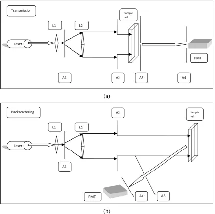
Using the diffusion assumption to describe the light propagation in strongly scattered medium largely simplifies the analysis of DWS measurement. Photons are scattered for multiple times, and then undergo a large number of intermediate scattering events. As a result, the scattering vector is not as much relevant to correlation function as that in DLS. Consequently, the importance of the scattering angle between incident and detected light in DLS has been reduced for DWS. Therefore, the experimental geometry for DWS can be diversified with various scattering angels. Besides the basic experimental geometry, transmission, the backscattering geometry has been developed by researchers [85, 88, 90].

Transmission experiment geometry is an experiment set-up in which the light source is incident into sample slab from an extended plane source, and then it is detected from the opposite side of the sample slab. Photons traverse the suspension and experience multiple scatterings during this process. Pine et al. have expressed the electric field autocorrelation function in transmission as[88]

 





 





1 2 0

1 * _* 1 2

0

sinh 6

L G

l _{L l}

     _{ }          (2.8)

where  is the diffusion constant, Lis the thickness of sample cell. When the decay time is much smaller than the characteristic diffusion time, that is ₀, Equation (2.8) can be re-written to[88]

 





 





1 2 * 0

1 _* _{1 2}

(40)

23

Backscattering is another commonly used geometry. In this geometry, the laser beam enters from one face of the sample. After the photons are fully scattered, the light intensity signal is collected by the detector that is placed at the same side of the incident light, but with an angel formed between the incident light and detected light. The electric field autocorrelation function collected at any points in the same side can be expressed as[88]

 









 





1 2

* *

0

1 * _* 1 2

0

sinh 6 1

1

1 _sinh ₆

L l l L

G

l L _{L l}

     _{ }  _          (2.10)

2.6 Summary

The particle’s dimension can be characterized using Feret’s diameter, Martin’s diameter, the projected area diameter, the maximum horizontal intercept, the perimeter diameter or other equivalent diameters dependent on the application of the particle. Dynamic light scattering is a well established method used commercially. It is able to measure the mean particle size (hydrodynamic particle size) and particle size distribution. The principle of DLS is to detect the light that, when going through a medium, will fluctuate with a characteristic time scale. The characteristic decay time provides valuable information about the dynamic medium, including particle size. Therefore, particle size can be derived from the measured correlation function. However, DLS is not robust enough to research the highly scattering medium due to the unknown scattering vector. It is limited in strictly single scattering system with a low particle concentration.

(41)

24

Chapter 3 Experimental Set-up and Arrangement

3.1 Introduction

A variety of methods are available to measure the dimension of an individual particle and the average size of collective particles [30, 55]. Depending on the techniques, different experimental methods have been developed for particle size measurement. DWS is a method developed from conventional DLS, therefore, their set-up and arrangement are similar. They are same in that a small sample slab filled with particle suspension is illuminated by a laser beam. The light photons are fully scattered in the sample medium, and then the intensity of the signal is collected by a detector. After that, the light signal is processed and displayed visually. Finally, the data is recorded by a computer and processed by program. Essentially, the system consists of a particle sample, a laser beam, a detector, a processor and a computer. It can be grouped in optical system and sample cell system. However, in order to meet specific requirements in applications, the set-up could vary in experimental geometry, equipment selection, and apparatus arrangement.

For traditional DWS, two different geometries (transmission and backscattering) can be used to increase its flexibility and practicality. Besides the geometries, choosing a proper device in DWS measurement is also important, especially the light signal detector. The Photomultiplier (PMT) tube was commonly used due to its high sensitivity, but the Charge-couple Device (CCD) camera has been becoming increasingly popular because of its ability to monitor a large number of speckles. The multi-speckle approach makes that the light signal’s ensemble average can be achieved, hence the data processing time can be reduced substantially.

(42)

25

3.2 Overview of DWS Experimental Set-up

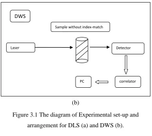
DWS is an improved method of DLS, which extended the ability of light scattering method to highly scattering system. As such DWS shares a number of features of the conventional DLS, particularly in the arrangement of optical system and the way of light signal data collection. However, there are some differences between the two methods. Figure 3.1(a) shows the basic experimental set-up of the classic DLS, in which a laser beam is incident into a small volume particle solution. Then, the light photons diffuse with several random walks till they escape from the solution and exit from the sample around the slab. The detector is applied to receive the photons, and to measure the fluctuation of light intensity. After the light fluctuation is processed by digital correlator, the data is ultimately output to a PC to be analysed. Figure 3.1(b) shows a typical DWS experimental set-up with transmission geometry. A coherent laser light is incident on the left face of a sample cell filled with particle solution. When the laser beam travels through the sample, photons are scattered by particles and then move along random paths in the solution. After a large number of scatterings, the photons escape from the suspension and are then collected by the detector located on the opposite side of the laser source. The optical waves received from different light paths reflect the fluctuation of light intensity. The intensity fluctuation is processed by a digital correlator to produce the autocorrelation function which is then exported to a computer.

(a) Laser

Detector

θ

Sample with index-match

correlator PC

(43)

26 (b)

It can be seen from the above that DWS set-up is different from DLS. The main differences are that DLS requires index-match which is matching the refractive index of both particle and solution to improve the optical object detection[91]; the light intensity fluctuation is sensitive to the angle of detector away from the axis, θ, as shown in Figure 3.1.

The basic DWS can be enhanced by adding apparatus. For example, Scheffold[40] developed a device as shown in Figure 3.2, which works for both geometries. Hence the light can be detected in both transmission and backscattering. A water reservoir is used to control temperature; in the mean time, it also works as an index matching solution for the sample cell mounted inside. Two polarizers are applied, one with λ/2 retardation plate aiming to retain a continuous variation of the incident light intensity from the laser, and the other working in backscattering allowing the detection of polarized or depolarized lights. The beam-expander controls the width of the laser beam, making it significantly larger than the thickness of the sample.

Laser Detector

Sample without index-match

correlator PC

DWS

[image:43.595.150.447.67.332.2]

(b) Figure 3.1 The diagram of Experimental set-up and

(44)

27

Figure 3.2 Diffusing-wave spectroscopy set-up which works for both transmission and back-scattering geometries[40].

Apart from polarizer, optical fibres can also be used in DWS. Keuren et al.[92] used the single-mode fibre for concentrated latex dispersion. The single-mode optical fibre is an optical fibre which only carries a single ray of light or a single mode of light. It was used to reduce the effect of autocorrelation function of multiple scattered lights from concentrated dispersions. Similar set-up is used in the experiment of Rojas-Ochoa et al.[93] which investigated the small-angel neutron scattering from concentrated colloidal suspension using a single mode fibre.

An experimental study of particle sizing in static condition and in shear flow by diffusing-wave spectroscopy