Identifying Taste Variation in Choice Models

This is a repository copy of Identifying Taste Variation in Choice Models. White Rose Research Online URL for this paper:

http://eprints.whiterose.ac.uk/2515/

Conference or Workshop Item:

Whelan, G.A. (2003) Identifying Taste Variation in Choice Models. In: European Transport Conference 2003, 8-10 Oct 2003, Strasbourg, France.

[email protected] https://eprints.whiterose.ac.uk/

Reuse

See Attached

Takedown

If you consider content in White Rose Research Online to be in breach of UK law, please notify us by

Universities of Leeds, Sheffield and York

http://eprints.whiterose.ac.uk/

Institute of Transport Studies University of Leeds

This is an author produced version of a paper given at the European Transport Conference, 2003. We acknowledge the copyright of the Association of

European Transport and upload this paper with their permission.

White Rose Repository URL for this paper: http://eprints.whiterose.ac.uk/2515

Published paper

Whelan, G.A. (2003) Identifying Taste Variation in Choice Models - European Transport Conference 2003, 8-10 October, Strasbourg, France.

IDENTIFYING TASTE VARIATION FROM CHOICE MODELS

Gerard Whelan

Institute for Transport Studies, University of Leeds

1. Introduction and Objectives

Among the many attractive features of the mixed logit model is its ability to take account of taste variation among decision-makers by allowing coefficients to follow pre-specified distributions (usually normal or lognormal). Whilst accounting for heterogeneity in the population, simple applications of the technique fail to identify valuable information on differences in behaviour between market segments. This information is likely to be of use to those involved in policy and investment analysis, product design and marketing.

The ‘standard’ approach to overcome this problem when working with the mixed logit model is to identify segments prior to modelling and either specify a set of constant coefficients for each market segment together with an additional error term to ‘mop-up’ any residual variation, or by allowing separate distributions for each market segment.

An alternative approach is to adapt an exciting new methodology that offers the ability to estimate reliable individual specific parameters (Revelt and Train, 1999). This approach is documented in Section 3 and involves three key stages:

• First use maximum simulated likelihood to estimate distributions of tastes across the population.

• Next examine individual’s choices to arrive at estimates of their parameters, conditional on know distributions across the population (including accounting for uncertainty in the population estimates). This process again involves the use of maximum simulated likelihood.

• Finally, differences in behaviour between market segments are identified by regressing individual ‘part-worths’ against the characteristics of the decision-maker or attributes of the choice alternatives.

In the first instance the technique is validated under ‘controlled’ circumstances on a simulated data set with know taste distributions. This simulation involves a binary choice situation in which the alternatives are described in terms of time and cost. The choices of a group of decision-makers are simulated with each with a value of time drawn from a known distribution. The resulting choices are then analysed and individual values recovered with a surprisingly high degree of precision. The findings of this validation are set out in Section 4.

specifications defined by purchase price, running costs, engine size, emissions and safety features. The results of this analysis are set out in Section 5 and are compared to the findings of previously calibrated models that identified significant differences in tastes across market segments.

2. Identifying Taste Variation Using ‘Traditional’ Methods

There are two well-documented approaches when using discrete choice models to examine taste variation across different market segments. The first involves an application of the likelihood ratio test and the second involves estimating specific coefficients for each segment (Ben-Akiva and Lerman, 1985). To undertake the likelihood ratio test we classify the data into market segments and estimate separate models with identical specifications for each segment. We then test the hypothesis that the coefficients are the same across segments.

G 2

1

0: ...

H β =β =β (1)

where β_gare the coefficients for market segment g, selected from the total of G segments

We reject the null hypothesis of equal coefficients if:

2 df g

G

1 g

Ng N(ˆ) L (ˆ )

L

2 _⎥ >χ

⎦ ⎤ ⎢

⎣ ⎡

β −

β

−

∑

=

(2)

Where L_N(βˆ) is the final log-likelihood of the pooled model

) ˆ (

L_Ng β_g is the final log-likelihood of the segment g model is the number of coefficients in the segment g model

g K

is the degrees of freedom

∑

=

−

G

1 g

g K K

df

The advantage of the likelihood ratio test is that it is simple to compute. However, if there are many segments, the number of observations for each model can become small and the application of the model to forecasting can become complex.

An alternative approach to the likelihood ratio test is to specify segment specific coefficients on the attribute values. This can be done in an absolute (equation 3) or incremental way (equation 4).

X D .. X D X D

U=β1 1 +β2 2 + +βG G (3)

X D .. X D X

U=β +β′2 2 + +β′G G (4)

Equation 4 shows the absolute specification in which a separate coefficient is estimated for each segment. To examine differences between segments the coefficients and standard errors should be compared using an asymptotic t-test:

) ˆ ˆ cov( 2 ) ˆ var( ) ˆ var(

ˆ ˆ

2 1 2

1

2 1

β β −

β + β

β − β

(5)

Equation 5 shows an incremental approach to testing market segments. Here, one or more segments are selected as the base and other segments are examined relative to the base. In the example shown in equation 5, the coefficient for the base segment is given by β and the coefficient for segment 2 is . In this case the appropriate statistical significance test is simply the t-statistic on the incremental coefficient, or if a series of incremental coefficients are used a likelihood ratio test is appropriate.

2

β′ + β

In the preceding analysis, a unit change in the value of an attribute is independent of the absolute level of the attribute, for example a £1 change in purchase price has the same impact of utility for a vehicle priced at £5,000 as a £1 change on a vehicle priced at £20,000. This restriction can be relaxed to some degree by the market segmentation analysis described above but a more general approach is to specify a utility expression that is non-linear. Although we can envisage many types of non-linear function (e.g. logarithmic, Box-Cox, quadratic), the power function specified in equation 6 has some very desirable properties.

γ β

= X

U (6)

If γ is equal to one the utility function is linear in response to changes in and if is less than 1 the impact of a change in is reduced as falls.

X X

γ γ

3. Identifying ‘Random’ Taste Variation Using the Mixed Logit Model

The mixed logit estimation procedures adopted in this section uses a specification suggested by Revelt and Train (1998) which states that an individual faces a choice among J alternatives in each of T time periods or choice situations. The utility that person n obtains from alternative i in choice situation t is:

nit nit n nit X

U =β′ +ε (7)

Where:

n

β is a vector of coefficients for individual n which varies in the

population with density f(β|θ) where θare the parameters of this distribution

nit

is an unobserved random error that distributed iid extreme value

nit

ε

If denotes the individual’s sequence of choices, then conditional

on the individual’s preferences (

nT 1 n n y ....y

y =

n

β ), the probability that individual n chooses alternative y_nt in time period t can be expressed by the logit model:

∑

β′ β′ = β j njt t ny nt nt ) X exp( ) X exp( ) | y ( L nt (8)

The unconditional probability is the integral of the conditional probability over all possible values of β.

∫

β ⋅ β θ β =

θ) L (y | ) f( | )d |

y (

Q_{nt nt nt nt} (9)

Assuming that the individual’s tastes do not change over choice situations, the conditional probability of individual n’s sequence of choices is the product of logits:

∏

β = β t nt nt

n| ) L (y | ) y

(

S (10)

The unconditional probability is:

∫

β ⋅ β θ β =

θ) S(y | ) f( | )d |

y (

P _{n n} (11)

The goal of the first stage of the estimation process is to estimate parameters that describe the distribution of tastes across individuals. Unlike the estimation of standard logit models exact maximum likelihood estimation is not possible since the integral in equation 11 cannot be evaluated analytically. Instead, a simulated likelihood function is specified in which P(y_n |θ) is approximated by summation over randomly chosen values of β. The process is repeated for R random draws of β (where βr is the r-th draw from f(β|θ)) and the simulated probability of the individual’s sequence of choices is:

) | y ( S ) R / 1 ( ) | y (

SP _n r

R

1 r

n θ =

∑

β

=

(12)

3.1 Individual Specific Tastes

Although we can estimate the density f(β|θ) describing the distribution of tastes in the population it is also desirable to know where each decision-maker is in this distribution. Following Revelt and Train (1999), let denote the density of conditional on the decision-maker’s sequence of choices and the population parameters . By Bayes’ rule:

) , y | (

gβ _n θ

β

θ

(

)

(

) (

(

θ

)

)

θ β ⋅ β = θ β | y P | f | y P , y | g n n n (13)

Equation 13 is then used to calculate the conditional expectation of β, the individual’s expected tastes k

( )

β .

(

k|y ,θ

)

=

_∫

k

( ) (

β ⋅gβ|y ,θ

)

dβ

E _{n n} (14)

Substituting the formula for g

(

)

( ) (

) ( )

(

)

( ) (

) ( )

(

β

) ( )

⋅ β θ β

β θ β ⋅ β ⋅ β = β β θ β ⋅ β ⋅ β = θ

∫

∫

∫

d | f | y P d | f | y P k | y P d | f | y P k , y | k E n n n n n (15)

As equation 15 does not have a closed form, the conditional expectation of β is approximated by simulation. This procedure involves taking random draws of β from the population density f(β|θ)and estimating the weighted average of these draws with the weight of the draw βr being proportional to P

(

y_n|βr

)

:

(

)

( ) (

)

(

)

∑

∑

β β ⋅ β = θ r r n r n r r n | y P | y P k , y | k

E~ (16)

4. Validation

[image:8.595.82.516.74.227.2]

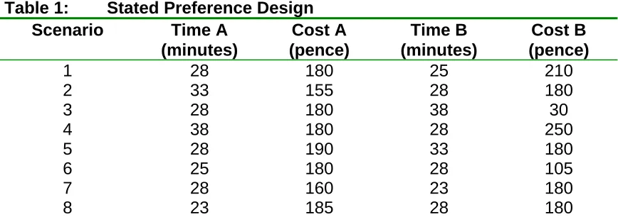
Table 1: Stated Preference Design

Scenario Time A

(minutes)

Cost A Time B Cost B

(pence) (minutes) (pence)

1 28 180 25 210

2 33 155 28 180

3 28 180 38 30

4 38 180 28 250

5 28 190 33 180

6 25 180 28 105

7 28 160 23 180

8 23 185 28 180

Each simulated individual has a value of time (pence per minute) drawn from a normal distribution for the population with a mean of 6 and a standard deviation of 2. The utility function for each choice alternative is specified as the negative of cost minus the value of time multiplied by the time plus a randomly normally distributed error term with a mean of zero and a standard deviation of 10. Individuals simulated choices are based on utility maximisation.

Table 2: Choice Models of Simulated Data

Logit Mixed logit

Cost -0.0964 (127.1) -0.1232 (113.0)

Time -0.5941 (125.8) -0.7395 (107.5)

Time (Standard Deviation) n.a. 0.2458 (60.8)

Number of Observations 80000 80000

Final Likelihood -30714.4 -28903.3

Value of Time (pence per minute) 6.16 6.00

Standard Deviation (pence per minute) n.a. 2.0

Note: both models were estimated in GAUSS using code developed by Kenneth Train. The Mixed logit model was estimated using 500 Halton draws.

The MNL and mixed logit choice models calibrated to this data are shown in Table 2. As expected, the MNL model is able to recover the mean value of time and mixed-logit model is able to recover the mean and standard deviation of the value of time across the sample. The next stage is to apply the methodology outlined in Section 3.1 to identify individual specific values of time.

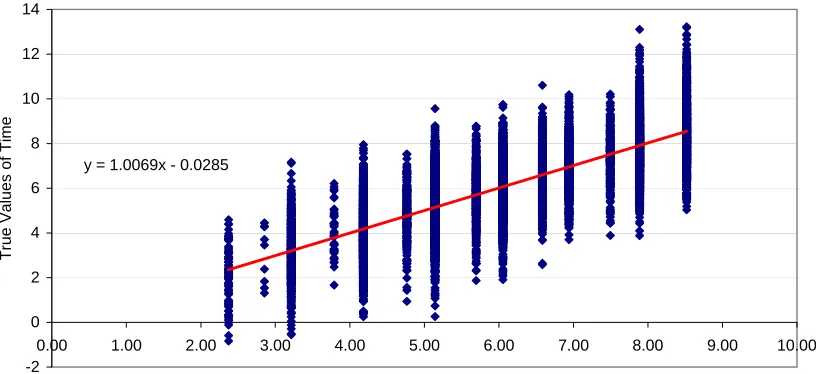
y = 1.0069x - 0.0285

-2 0 2 4 6 8 10 12 14

0.00 1.00 2.00 3.00 4.00 5.00 6.00 7.00 8.00 9.00 10.00

Estimated Values of Time

[image:9.595.98.506.83.270.2]

True Values of Time

Figure 1: Scatter of Actual and Estimated Values of Time

Bearing in mind that because the SP design offers a limited number of trade-offs the estimated values are clustered in groups defined by the implicit boundary values of time the technique looks very promising indeed. The next task is to apply the approach to a real data set.

5. Identifying Taste Variation in Preferences of Vehicle Type

As part of an Engineering and Physical Science Research Council funded project aimed at developing multi-modal travel forecasts for Great Britain, a stated preference survey was undertaken to help understand how price and running costs influence the household’s choice of vehicle type. The survey design, reported in Whelan (2003), involved the use of two separate SP experiments looking at the influence of purchase price, running costs, engine size, emissions and safety features on the choice of vehicle type. The five vehicle attributes were combined to generate two separate SP experiments in which the respondent was asked to state a preference between two hypothetical vehicle specifications (vehicle A and vehicle B):

• SP1 examines the trade-off between Running Costs, Vehicle Emissions and Safety Features.

• SP2 examines the trade-off between Purchase Price, Running Costs and Engine Size.

Using information on the household’s existing vehicle fleet and the respondent’s stated intentions about future ownership, the experiments were customised for each individual respondent so that the choice context was relevant. The respondent was told to assume that all other attributes were identical between specifications.

initially contacted by letter and invited to participate in the study. Householders who were willing to participate in the study and had just or were about to acquire a car were visited in their homes and presented with the questionnaire mounted on a laptop computer. A computer-assisted survey was undertaken since it was necessary to customise the SP design for each respondent. Data from a total of 329 households was collected during October and November 1998.

5.1 MNL Model Calibration

The starting point for analysis was a simple MNL model for each experiment taking the choice of vehicle as a function of the vehicle attributes presented in the designs. As respondents were told to assume that all other vehicle attributes were identical between vehicles we did not expect nor did we find statistically significant alternative specific constants. Although the models are not reported here, it is useful to note that each showed a very good level of fit (ρ2 statistics with respect to constants of 0.4503 and 0.2543 for SP1 and SP2 respectively) and all coefficients had the expected sign and were statistically significant at the usual level (before adjusting for repeat observations). Having developed useful models for each experiment, the next stage to model estimation was to merge the two datasets and estimate a single model.

[image:11.595.79.520.73.396.2]

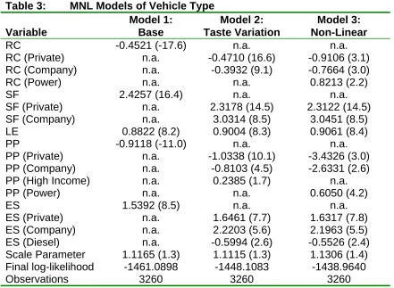
Table 3: MNL Models of Vehicle Type

Model 1: Model 2: Model 3:

Variable Base Taste Variation Non-Linear

RC -0.4521 (-17.6) n.a. n.a.

RC (Private) n.a. -0.4710 (16.6) -0.9106 (3.1)

RC (Company) n.a. -0.3932 (9.1) -0.7664 (3.0)

RC (Power) n.a. n.a. 0.8213 (2.2)

SF 2.4257 (16.4) n.a. n.a.

SF (Private) n.a. 2.3178 (14.5) 2.3122 (14.5)

SF (Company) n.a. 3.0314 (8.5) 3.0451 (8.5)

LE 0.8822 (8.2) 0.9004 (8.3) 0.9061 (8.4)

PP -0.9118 (-11.0) n.a. n.a.

PP (Private) n.a. -1.0338 (10.1) -3.4326 (3.0)

PP (Company) n.a. -0.8103 (4.5) -2.6331 (2.6)

PP (High Income) n.a. 0.2385 (1.7) n.a.

PP (Power) n.a. n.a. 0.6050 (4.2)

ES 1.5392 (8.5) n.a. n.a.

ES (Private) n.a. 1.6461 (7.7) 1.6317 (7.8)

ES (Company) n.a. 2.2203 (5.6) 2.1963 (5.5)

ES (Diesel) n.a. -0.5994 (2.6) -0.5526 (2.4)

Scale Parameter 1.1165 (1.3) 1.1115 (1.3) 1.1306 (1.4)

Final log-likelihood -1461.0898 -1448.1083 -1438.9640

Observations 3260 3260 3260

Notes:

All t-statistics are shown with respect of zero except the scale parameter and the power coefficients, which are shown with respect to one.

Running Costs (RC) are in pence per mile, 1998 values

Safety Features (SF) are ABS brakes, side impact protection bars and driver airbags Low Emissions (LE) – this engine produces fewer emissions than the standard engine Purchase Price (PP) is in £K, 1998 values

Engine Size (ES) is in litres

Additional examination of respondents’ preferences was undertaken using non-linear utility expressions incorporating power terms (shown in equation 6) on running costs and purchase price. Separate coefficients were initially specified for private and company buyers but these were subsequently combined, as they were not statistically significant from each other. Both power terms are below unity and imply that a unit change in running cost or purchase price has a lower impact on choice the higher the running costs or purchase price respectively. This model is shown as Model 3 in Table 3.

The preferred model (Model 3 in Table 3) shows a good level of overall fit as demonstrated by a ρ2 statistic with respect to constants of 0.3632, statistically significant coefficients with correct signs and reasonable magnitudes. More specifically, the model indicates the following.

The higher the purchase price the less likely the car is to be chosen and that private buyers are more sensitive to price than company buyers. The power term on price indicates that the impact of a unit change in the price of the vehicle is proportionally less for high priced vehicles than for low prices vehicles. This may be because higher priced vehicles are typically bought by high-income customers who according to Model 2 are less sensitive to price change.

The higher the running costs the less likely the car is to be chosen. Comparing the coefficient for running costs with that for purchase price indicates that a private individual spending £9,880 on a new car (the average in the sample) would be willing to pay £547 more to receive a penny per mile reduction in running costs on a vehicle with an average running cost of 15.2 pence per mile. Under the same assumptions, similar calculations show the company buyer to be willing to pay £600 for a penny reduction in running costs.

The marginal monetary valuation of running costs for private buyers is obtained by estimating the ratio of the marginal utility of running costs over the marginal utility of purchase price1:

5472 . 0 880 . 9 * 4326 . 3 * 6050 . 0 2 . 15 * 9106 . 0 * 8213 . 0 PP U RC U MU MU ) 1 6050 . 0 ( ) 1 8213 . 0 ( PP RC = − − = ∂ ∂ ∂ ∂

= −₋ (17)

Assuming an annual mileage of 10,000, the private respondent will take 5.5 years to break even, whereas using an assumption of 15,000 miles per annum, the respondent will take 3.6 years to break even.

Buyers prefer vehicles with a higher safety specification, with private buyers willing to pay £2752 and company drivers willing to pay £4724. These values are arguably too high and may have arisen as a result of respondent bias. Vehicles with high safety specifications tend to be better quality vehicles in general and although the respondent was asked to assume that all other vehicle

1

attribute were equal, the high safety value may also be picking up other quality effects.

Private buyers prefer low emissions vehicles to standard vehicles less than company buyers with each willing to pay £1078 and £1406 respectively.

In the acquisition of company vehicle, higher engined vehicles are preferred to smaller engined vehicles with buyers willing to pay £3.40 per cc for petrol cars and £2.54 for diesel cars. Private buyers also like larger cars and would be willing to pay £1.94 per additional petrol cc and £1.28 per additional diesel cc.

With the exception of the coefficient on safety features, the model results and relative values look quite plausible. The next task is to see if the logit models can be improved using more sophisticated mixed-logit techniques.

5.2 Mixed Logit Approach

It was noted in Section 5.1 that in order to merge data from the two SP experiments to develop a single choice model, allowance must be made for differences in ‘scale’ between the two data sets. In the context of the development of logit models this was done using the artificial tree structure proposed by Bradley and Daly (1991). However, when developing mixed-logit models, differences in scale are accommodated by adding normally distributed error components to the utility functions for each option in the experiment with the most error, and setting its mean value to equal zero (Brownstone et al, 2000). A scale parameter greater than unity in the estimation of joint logit models (Model 1 in Table 3) indicates that SP1 has the greater random error and hence the mixed-logit specification is represented by the following utility functions:

nit i nit 1

SP nit X

U =β +η +ε (18)

nit nit 2

SP

nit X

U =β +ε (19)

Where:

is a vector of coefficients constrained to be equal across individuals, alternatives and periods

β

is a vector of explanatory variables

X

is a normally distributed random error with a mean zero and standard deviation . The errors are independent error across alternatives in the experiment with the greatest error but their standard deviations are constrained to be equal.

η

2

σ

ε is a Gumbel error term that is independently identically distributed across individuals, alternatives and periods

[image:14.595.78.521.100.327.2]

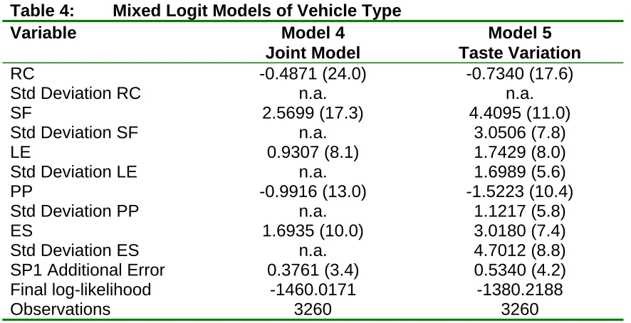
Table 4: Mixed Logit Models of Vehicle Type

Variable Model 4 Model 5

Joint Model Taste Variation

RC -0.4871 (24.0) -0.7340 (17.6)

Std Deviation RC n.a. n.a.

SF 2.5699 (17.3) 4.4095 (11.0)

Std Deviation SF n.a. 3.0506 (7.8)

LE 0.9307 (8.1) 1.7429 (8.0)

Std Deviation LE n.a. 1.6989 (5.6)

PP -0.9916 (13.0) -1.5223 (10.4)

Std Deviation PP n.a. 1.1217 (5.8)

ES 1.6935 (10.0) 3.0180 (7.4)

Std Deviation ES n.a. 4.7012 (8.8)

SP1 Additional Error 0.3761 (3.4) 0.5340 (4.2)

Final log-likelihood -1460.0171 -1380.2188

Observations 3260 3260

Notes:

All t-statistics are shown with respect to zero.

Both models were estimated using 500 Halton draws. Running Costs (RC) are in pence per mile, 1998 values

Safety Features (SF) are ABS brakes, side impact protection bars and driver airbags Low Emissions (LE) – this engine produces fewer emissions than the standard engine Purchase Price (PP) is in £K, 1998 values

Engine Size (ES) is in litres

Having allowed for a difference in scale between the two data sets, the next stage to model development is to allow for heterogeneity in tastes among individuals in the sample. In the calibration of the GEV models this was done using market segmentation analysis and non-linear relationships in sensitivity to attribute levels. In the mixed logit model taste variation is accounted for by specifying additional random coefficients of the form:

nit i nit nit

nit X X

U =β +ξ +η +ε (20)

Where:

is a vector of coefficients constrained to be equal across individuals, alternatives and periods

β

is a vector of coefficients which show the standard deviation around the mean of the random coefficients specified in vector β

ξ

is a vector of explanatory variables

X

is a normally distributed random error with a mean zero and standard deviation . The errors are independent error across alternatives in the experiment with the greatest error but their standard deviations are constrained to be equal.

η

2

σ

Normally distributed random coefficients were detected using the Lagrange Multiplier test, as specified by McFadden and Train (2000). This test showed that there were significant random components on all coefficients and this was confirmed with estimation of the mixed logit.

Following recommendations from Brownstone et al (2000), it is advisable to keep at least one coefficient fixed during estimation and as running costs will be used to link the RP and SP models, this coefficient is estimated as a fixed value. Coefficients on safety features, low emissions, purchase price and engine size were all specified to be normally distributed. The results are shown as Model 5 in Table 4.

Estimates of the standard deviation of the behavioural coefficients show a considerable degree of taste variation across the sample. The coefficients indicate that in general, respondents prefer the inclusion of safety features, low emissions, lower purchase price and higher engine sizes but the size of the standard deviations imply that some respondents show counter intuitive preferences: 7.4% of the distribution prefer not to have safety features, 15.2% are against low emissions, 8.7% prefer higher prices and 26.1% prefer smaller engines. The large standard deviation on engine size is plausible. Whilst the majority of respondents favour larger engined vehicles there is a substantial minority who associate a disutility with large engined cars. In reality it is likely that owners have an ideal engine size to perform the majority of tasks that the vehicle will be used for and that a movement away from this ideal leads to a reduction in utility. It is possible to avoid ‘wrong’ signed coefficients using log-normal distributions but this restriction reduces the overall goodness of fit and given that only a small proportion of the data showed counter intuitive responses the normally distributed coefficients were considered appropriate.

The preferred mixed logit model (shown as Model 5 in Table 4) accounts for a potential difference in scale between the two choice experiments and accounts for differences in tastes between individuals.

In terms of overall fit, allowing for taste variation generates substantial improvements over traditional MNL models and coefficient estimates show the following.

Brownstone et al (2000) note that as the MNL is a nested special case of the mixed logit, the two models can be compared using a likelihood ratio test. Comparing Model 3 with Model 5 gives a highly significant likelihood ratio statistic of 117.49 with 3 degrees of freedom. The mixed logit models therefore appear to outperform the equivalent GEV models in terms of fit. A direct comparison of the coefficients from the GEV and mixed logit models is not possible because the stochastic portion of utility is different in each and the two models have different scales so we can only compare the relative (monetary) value of attributes. This is done in Table 5 in which the mixed logit model appear to generate lower relative values for running cost, safety features and emissions but the difference is less marked for engine size.

Table 5: Average Relative Attribute Values (£)

Mixed Logit MNL (Private) MNL (Company)

Running Costs 482 547 600

Safety Features 2897 2752 4724

Low Emissions 1145 1078 1406

Engine Size 3.09 1.94 3.40

5.3 Identifying Individual Specific Values

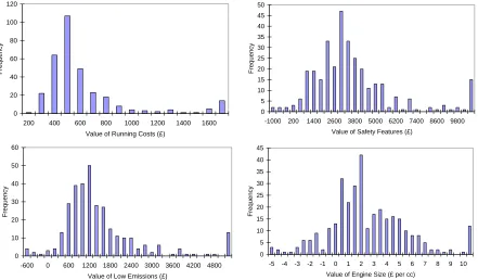
The final stage to the identification of preferences was to apply the methodology set out in Section 3.1 to estimate household specific values for each of the vehicle attributes. Histograms of household specific estimates of the relative attribute values are presented below.

0 20 40 60 80 100 120

200 400 600 800 1000 1200 1400 1600 Value of Running Costs (£)

F

requency

0 5 10 15 20 25 30 35 40 45 50

-1000 200 1400 2600 3800 5000 6200 7400 8600 9800 Value of Safety Features (£)

F

requenc

y

0 10 20 30 40 50 60

-600 0 600 1200 1800 2400 3000 3600 4200 4800 Value of Low Emissions (£)

Fr

equenc

y

0 5 10 15 20 25 30 35 40 45

-5 -4 -3 -2 -1 0 1 2 3 4 5 6 7 8 9 10 Value of Engine Size (£ per cc)

F

requenc

[image:16.595.84.525.436.694.2]

y

Figure 2: Histograms of Relative Attribute Values

were regressed against the socio-economic characteristics of households, clear patterns to this variation would emerge. This however was unsatisfactory as the results simply confirmed the dichotomy in tastes between company and private buyers and a marginal reduction in the sensitivity to purchase price, the higher the absolute level of the variable. It is therefore concluded that preferences for different vehicle types are diverse and not easily grouped. The values may however be related to other socio-economic characteristics not collected during the survey and this might be explored further using latent class models.

6. Conclusions

This paper reviews traditional approaches to the identification of taste variation within discrete choice models and reports on a new methodology to identify individual specific preferences (Revelt and Train, 1999). The new methodology was validated on simulated data before being applied to a real stated preference data set examining households’ preferences for alternative vehicle types. On the basis of the simulation testing, the methodology performs very well indeed, however, when applied to an actual data set the approach did not yield significantly more insight into how tastes vary across the population when compared with traditional methods. There are many instances in which information on individual preferences could generate improvements to policy, product design and marketing and on the basis of the research reported here this new approach has much to recommend.

References

Aptech Systems (1996) GAUSS Mathematical and Statistical System Maple Valley WA.

Ben-Akiva, M.E. and Lerman, S.R. (1985) ‘Discrete Choice Analysis’, The MIT Press, Cambridge, Massachusetts.

Ben-Akiva, M. and Morikawa, T. (1990) ‘Estimation of Switching Models from Revealed and Stated Intentions’, Transportation Research – Part A, Volume 24A, number 6, pp485-495.

Bhat, C (2000) ‘Quasi Random maximum simulated likelihood estimation of the mixed multinomial logit model’ Transportation Science, Vol 34, pp 228-238.

Bradley, M. and Daly, A.J. (1992) ‘Uses of the Logit Scaling Approach in Stated Preference Analysis’, 6th World Conference on Transport Research, Lyon, France, July 1992.

Brownstone, D., Bunch, D., and Train, K. (2000) ‘Joint Mixed Logit Models of Stated and Revealed Preferences for Alternative-Fuel Vehicles’, Transportation Research - Part B, Volume 34, pp315-338.

Revelt, D. and Train, K. (1998) ‘Mixed Logit with Repeated Choices: Households’ Choice of Appliance Efficiency Level’, Review of Economics and Statistics. Vol LXXX, No 4, pp 647-657.

Revelt, D. and Train, K. (1999) ‘Customer-Specific Taste Parameters and Mixed Logit’ http://elsa.berkeley.edu/wp/train0999.pdf.

Train, K. (1999) ‘Halton Sequences for Mixed Logit’, Department of Economics, University of California, Berkeley.

Train, K. (2002) ‘Discrete Choice Methods with Simulation’, Cambridge University Press, Scheduled publication date Autumn 2002.