Unequally Spaced Linear Antenna Array Synthesis with Minimum Side Lobe Levels Using Modified Differential Evolution Algorithm

(1)

International Journal of Innovative Technology and Exploring Engineering (IJITEE) ISSN: 2278-3075, Volume-8 Issue-7, May, 2019



Abstract: Antenna arrays are popularly used in various applications which include satellite, radar, wireless and cellular mobile communications etc. The present day communication systems performance greatly depends on the efficient design of antenna array systems. To meet the demands of noise free communications, it is required to design the antenna arrays with low side lobe levels (SSL). In this paper, a modified version of differential evolution (DE) algorithm is proposed to synthesize the linear antenna arrays with minimum side lobe levels. The mutation part of the traditional DE has been modified by adopting the normal mutation parameter. The various linear antenna arrays (10, 20 and 28 element) have been considered for the synthesis. The proposed modified DE (MDE) along with traditional DE algorithm and particle swarm optimization (PSO) algorithms have been applied. All the algorithms are applied to optimize the position between the elements. The numerical illustrations illustrate that the proposed method is out performed the traditional DE and PSO in terms of low side lobe level and convergence rate. From these results it is demonstrating that MDE is best suitable candidate for the optimization problems.

Index Terms: Convergence rate, differential evolution, linear antenna array, MDE, PSO, side lobe levels.

I. INTRODUCTION

The main objective of array antenna pattern synthesis is to approximate the desired radiation pattern by controlling the antenna array elements positions and by varying excitation currents amplitudes and phases to each antenna element. The optimization algorithms used for antenna arrays synthesis are either stochastic or deterministic. In antenna array synthesis problem stochastic optimization algorithms widely used because these algorithms can easily escape from local minima [1], [2].

Antenna array synthesis can be achieved by both deterministic and stochastic optimization algorithms. The deterministic optimization algorithm performs calculations over regions of the solution space, whereas the optimization algorithm performs calculations on single points.Most of the case stochastic optimization algorithms for example, genetic algorithm (GA) [3], DE algorithm [4], PSO algorithm [5], [6], bees algorithm [7], tabu search algorithm [8], ant colony

Revised Manuscript Received on May 07, 2019.

S.Venkata Rama Rao, Ph.D scholar, JNTUK, Kakinada, India.

A.Mallikarjuna Prasad, Professor of ECE, University College of Engineering, JNTUK, Kakinada, India.

Ch.Santhi Rani, Professor, ECE department, USHA RAMA College of Engineering and Technology, Telaprolu, near Gannavaram, India.

optimized (ACO) algorithm [9], cat swam optimization algorithm [10] and so on out performs deterministic optimization algorithms in antenna array synthesis problems. In recent years unequally spaced or aperiodic array antennas are wide spread in radar communication and satellite communication (SATCOM). If the periodicity in antenna array is changed, the aperiodic antenna array suppresses the sidelobe levels to minimum level. Different methods of synthesis of antenna arrays are presented to reduce the SLL to minimum level [11]. In unequally spaced arrays main beam can be steered over a larger frequency bandwidth compared with an equally spaced array. The unequally spaced antenna arrays can be classified into thinned and nonuniform arrays depending on whether the number of array elements is fixed or not [12]. The number of elements in the thinned arrays is not fixed. But in unequally-spaced arrays the number of array elements is fixed and the positions of elements are optimized with a real vector. In this paper a modified DE algorithm is proposed for synthesis of nonuniform arrays.

II. PATTERNSYNTHESISOFLINEARANTENNA ARRAY

We assume linear array geometry as shown in Fig. 1 with symmetrically placed 2N isotropic antenna elements along x axis.

Fig.1. Symmetric linear array geometry A. Array Factor of linear array

Antenna arrays can be realized by simply looking into its radiation pattern and can be obtained from its array factor (AF).

Unequally Spaced Linear Antenna Array

Synthesis with Minimum Side Lobe Levels

Using Modified Differential Evolution

Algorithm

(2)

In general AF is depends on number of elements in the array, separation distance between adjustment elements and the weights used for relative excitation of the current magnitudes and phases. The array factor for the 2N-element linear antenna array the array factor at an arbitrary angle θ can be expressed as [2]





 sin 

,

, ,

n n

N

j kx n

n N

AF I X

 

I e

 







(1)

Where I represent amplitude excitation vector, X is the array element positions vector and ϕ is the vector of excitation phases, In andϕn represents the current excitation

and element phase, which is positioned at xn. And the wave

vector of incident wave with wavelength λ is k = 2π/λ

B. Peak Side Lobe Level (PSLL)

In array radiation pattern the side lobe levels cause the wastage of energy and are usually unwanted. In most applications of antenna arrays, these side lobe levels needs to be suppressed without changing the main beam the gain. The peak side lobe level can be expressed as [1]





_





_

0

AF

,

, ,

,

max

AF

,

, ,

S

I X

PSLL I X

I X



 



 

 



(2)

Where S is the space spanned by the angle θ not including main lobe with the center at θ0. Compared to amplitude and

phase excitation techniques, amplitude excitation minimizes cost of the system [1], [2]. For the uniform excitation of amplitude, the excitation current of all elements In is assumed

to be 1.0 and for uniform phase excitation ϕn = 0.

Hence, AF in equation (1) can be modified as





 sin 

,

n

N j kx

n N

AF X



e









(3)

Consequently, equation (2) becomes

 







0



AF

,

max

AF

,

S

X

PSLL X

X



 



(4)

Where, θ0 is considered to be 00.

III. DIFFERENTIALEVOLUTION(DE)

The Differential Evolution like genetic algorithm is the population based metaheuristic algorithm. In 1995 the DE algorithm is invented by Storn and Price uses the fundamental operations mutation, crossover and finally selection similar to GA algorithm. Unlike GA algorithm DE uses only the mutation as the primary search operation.

A. Classic Differential Evolution

Classic Differential Evolution (CDE) algorithm starts with a population of Np individuals. It optimizes an objective

function by initialization and evolution processes. First the initial population P0 is generated by initialization process. Then the evolution process of population is carried out from the generation Pn to Pn+1generation until final conditions are

attained. In the evolution process from generations Pn to Pn+1 the mutation, crossover and selection operations are performed one by one.

(a) Differential Mutation: In DE algorithm after initialization process a mutant vector or donor vector is produced with differential mutation operator. Then in each generation this donor vector is combined with parent vector to produce trial vector. Differential mutation creates a mutant vector Xn+1,v,i given as [1]



, 1 , 2



1, , , , 1

y y

n p n p

n v i n b i

y y

X



X

F

X











(5)

1  

i

p

₁_y



p

₂_y



N

_p

Where, the mutation intensity Fy is a positive real number

in [0, 1]. The optimization parameters vector for the mutation base bn,i is Xn,b,i . And p1y and p2y are integer

numbers.

(b) Crossover: Next the child vector Cn+1,i is generated through crossover operator. The variants of DE algorithm commonly use two basic crossover methods such as explicitly exponential crossover and binomial (or uniform) crossover. In uniform crossover the child vector Cn+1,i is generated according to the following formula [1]:

1, , 1,

1, ,

,

r

n v i n i

j j

n c i

j n i

j

x

c

x

otherwise



  

_{ }









(6)

Where and Cr is the control parameter of DE algorithm is

constant in the range [0, 1] and



nj 1,i



is random number.

(c) Selection: The DE algorithm uses selection process to determine surviving of the target vector to subsequent generation. In the selection process the value of the objective function for every trial vector f(Xn+1,c,i) is compared with its related target vector f(Xn,i) and the vector corresponding to better fitness value will continue to the next generation. The selection operation mathematically expressed as [1]



  



  

1, 1, , ,

1,

, 1, , ,

n i n c i n i

n i

n i n c i n i

c

f X

p

f X

   







 





(7)

B. Dynamic Differential Evolution

(3)

In most cases DDE algorithm outperforms the classic DE algorithm.

C. Differential Mutation

The differential mutation best value expressed mathematically as [1]



, 1 , 2



, 1, ,

1

y y

b n p n p

n p

n v i

y y

X



X

F

X











(8)

1  

i

p

₁_y



p

₂_y



p

_b



N

_p

Where

_X

n p, b_{is the optimization parameters vector of}

individual

_p

n p, b

and is randomly chosen from

p

n by satisfying the condition,



,





,1

 

, 2



min

y

,

y

b n p n p

n p

y

f X









_

_

(9)

IV. MODIFIEDDIFFERENTIALEVOLUTION ALGORITHM

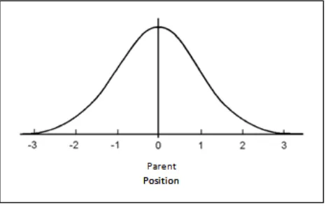
[image:3.595.52.285.463.610.2]

In MDE, we have replaced the traditional position updating equation by adopting the normal mutation mechanism. Normal mutation permits equal likelihood of movement in the positive and negative ways around the parent position. The modified DE updates the positions of the parent population using normal distribution. It is the major difference compared to the traditional DE. This step permits the DE to have a smaller (Large probability) and as well as larger mutations (Low probability) in the neighbourhood of parent position in a more systematic way.

Fig. 2. Normal Distribution Curve

Fig.2 shows the normal distribution curve. In this normal mutation approach smaller mutations are good turned over larger ones. The normal distribution density function mathematically expressed as





2 2

( ) 2 2

1 ; ,

2

normal

x

f

x

e

 



 



(10)

Where, μ is mean and σ standard deviation. The normal random number (N) following the above normal law is given

as



2



 

,

0,1

NM

 

 

 

NM

(11)

For the normally distributed random number NM (0,1), mean is zero and standard deviation is 1. By using the aforementioned equations, the updated position is defined by using the normal mutation random number. Therefore, for every dimension the position of ith population is updated as

 

, , , ,

1, ,

[

*

0,1 ]

n b i n b i

n v i

X

_



X



SF X

N

(12)

Where Xn,b,i the previous position of the population, σ is standard deviation and SF is the scaling factor.

V. SIMULATIONRESULTS

In this paper MDE algorithm is proposed to synthesize the linear array antennas for obtaining lowest side lode levels. This design requirement is achieved with MDE algorithm by optimizing the array element positions. Various linear array configurations with uniform amplitude and phase excitations are considered for analysis. The final results obtained with MDE algorithm are compared with non-optimized conventional array, PSO and DE optimized antenna array configurations. The parameter values assumed for both DE and MDE algorithms are number of population NP=50, crossover rate (CR) is 0.5 and scaling factor (SF) is 0.9. For PSO algorithm both C1 and C2 are taken as 2, population size

of 50 and

r



[0,1]

. Each of these two algorithms is executed 10 times. For each run 300 generations are considered and the radiation pattern is obtained with 1200 angles. And the azimuth angular region is considered between the angles 00 to 1800.The element position optimised with PSO, DE and MDE algorithms are shown in table 1 and the optimized array parameters in terms of PSLL and FNBW are shown in table 2. All the calculations are carried out using MATLAB R2015a on a system at operating 1.7 GHz with 4GB RAM.

5.1 Design examples for optimizing lowest SLL

In antenna arrays the side lobes represent unwanted radiation in unwanted directions. These side lobe levels of linear antenna array are to be optimized to the lowest levels by choosing optimum position in the antenna array.

The fitness function consider for this analysis minimizes maximum peak side lobe level and is achieved by [6]:

 

20 log

AF

Fitness

Min Max

Max AF



















_



_



_

_







(13)

(4)

[image:4.595.40.548.82.382.2]

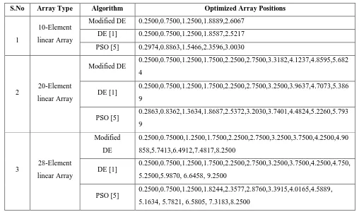
Table 1.Optimized antenna element position by using MDE, DE and PSO algorithms

S.No Array Type Algorithm Optimized Array Positions

1

10-Element

linear Array

Modified DE 0.2500,0.7500,1.2500,1.8889,2.6067

DE [1] 0.2500,0.7500,1.2500,1.8587,2.5217

PSO [5] 0.2974,0.8863,1.5466,2.3596,3.0030

2 20-Element

linear Array

Modified DE 0.2500,0.7500,1.2500,1.7500,2.2500,2.7500,3.3182,4.1237,4.8595,5.682 4

DE [1] 0.2500,0.7500,1.2500,1.7500,2.2500,2.7500,3.2500,3.9637,4.7073,5.386 9

PSO [5] 0.2863,0.8362,1.3634,1.8687,2.5372,3.2030,3.7401,4.4824,5.2260,5.793 9

3 28-Element

linear Array

Modified

DE

0.2500,0.75000,1.2500,1.7500,2.2500,2.7500,3.2500,3.7500,4.2500,4.90

858,5.7413,6.4912,7.4817,8.2500

DE [1] 0.2500,0.7500,1.2500,1.7500,2.2500,2.7500,3.2500,3.7500,4.2500,4.750, 5.2500,5.9870, 6.6458, 9.2500

PSO [5] 0.2500,0.7500,1.2500,1.8244,2.3577,2.8760,3.3915,4.0165,4.5889, 5.1634, 5.7821, 6.5805, 7.3183,8.2500

Table 2.Optimized antenna parameters in terms of PSLL and FNBW by using DE and MDE algorithms

S.No Array Type Algorithm

PSLL (dB) FNBW (Degrees)

Original PSLL

Optimized PSLL

Original FNBW Optimized FNBW

1 10-Element linear Array

Modified DE

-12.9681

-17.8364

23.6

22.4

DE [1] -16.4753 22.8

PSO [5] -15.0665 18.4

Modified DE

-13.1894

-19.6731

12

11.6

DE [1] -18.4251 11.6

PSO [5] -16.0132 10.4

Modified DE

-13.2353

-20.6105

8.4

DE [1] -18.5168 8.8

PSO [5] -17.4733 8.0

Example 1

A linear array of 10 elements is considered for obtaining SLL with minimum value in the angular region of θ = [00

, 790] and θ = [1010, 1800]. Then array pattern synthesised with MDE algorithm is compared with conventional and DE, PSO optimised array patterns. From Fig.3 it is observed that the reduction in the SLL with MDE algorithm is improved than conventional DE and PSO optimized array patterns. The SSL with proposed MDE algorithm is reduced by about 4.87dB from −12.96 dB to−17.83dB as compared with conventional array pattern. From table 2 it is also observed that the PSLL is reduced by about 3.51dB, 2.10dB with DE and PSO optimized patterns as compared with conventional

[image:4.595.43.546.415.592.2]

(5)

Fig.3. Normalized array factor of linear antenna array with 10 elements.

Fig.4. Convergence plot of fitness function of 10-element linear array using MDE Algorithm

Fig.5. Convergence plot of fitness function of 10-element linear array using DE Algorithm

Fig.6. Convergence plot of fitness function of 10-element linear array using PSO Algorithm

The convergence properties linear array with 10 elements by using MDE, DE and PSO are shown in the figures 4, 5 & 6 respectively.

Example 2

In this example MDE algorithm is applied to 20 element uniform linear array with element spacing of 0.5 λ. As compared to conventional array pattern the SLL of MDE pattern is reduced by 5.86 dB from −13.23 dB to −19.09 dB in the angular region of θ = [00

, 84.40] and θ = [95.60, 1800]. And as compared to DE pattern the SLL is reduced by 1.3 dB from −17.8 dB to −19.09dB as shown in Fig.7.

Fig.7. Normalized array factor of linear antenna array with 20 elements.

Fig.8. Convergence plot of fitness function of the 20-element linear array using MDE Algorithm

(6)

Fig.10. Convergence plot of fitness function of 20-element linear array using PSO Algorithm

The convergence properties of linear array with 20 elements by using MDE, DE and PSO are shown in the figures 8, 9 & 10 respectively.

Example 3

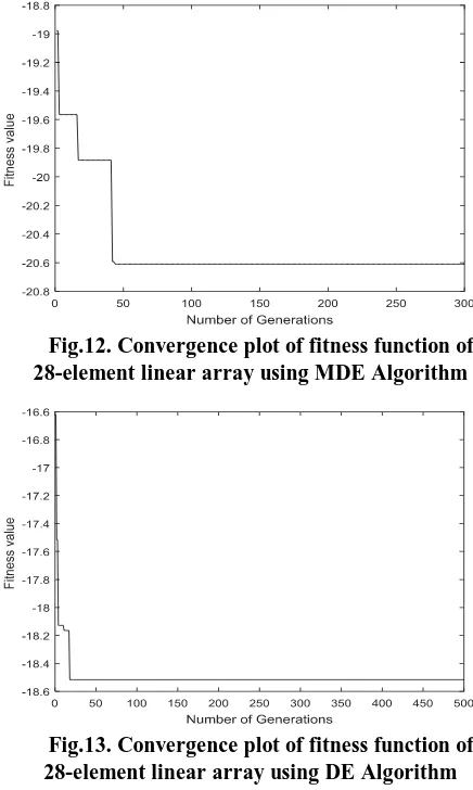
In the third example the 28 elements linear array is consider for minimum SLL value in angular region of θ = [00, 860] and θ= [940, 1800]. It seen from Fig.11, that the SSL obtained with proposed MDE algorithm is decreased by about 7.37dB, 2.09dB and 3.14 dB when compared with conventional, DE and PSO optimized array patterns respectively. The convergence properties of 28 element linear array by using MDE, DE and PSO are shown in the Figs. 12, 13 & 14 respectively.

[image:6.595.311.529.60.424.2]

Fig 11. Normalized array factor of 28 element linear antenna array.

Fig.12. Convergence plot of fitness function of 28-element linear array using MDE Algorithm

Fig.13. Convergence plot of fitness function of 28-element linear array using DE Algorithm

Fig.14. Convergence plot of fitness function of the 28-element linear array using PSO Algorithm 5.2. Convergence property of MDE Algorithm

It can be observed that from all the convergence plots the proposed MDE convergence rate is faster than the DE and PSO in achieving the lower PSLL levels.

VI.CONCLUSION

[image:6.595.54.277.60.234.2]

(7)

The algorithms DE, PSO and proposed MDE are applied to linear antenna array synthesize by optimizing array element positions. Numerical illustrations demonstrated that the MDE outperformed traditional DE and PSO. It can be seen that –17.83dB PSLL has been obtained by using MDE algorithm whereas –16.47dB and –15.06dB obtained by using traditional DE and PSO optimization algorithms for linear antenna array of 10 elements. There is a significant reduction of SLL of –1.36dB and –2.77dB when compared to DE and PSO optimised algorithms. For the 20 element linear array by using MDE algorithm, there is a significant reduction of –1.25dB and –3.66dB compared to the traditional DE and PSO. The PSLL of -19.67dB is obtained by using MDE algorithm whereas –18.42dB and –16.01dB are the PSLLs obtained by using traditional DE and PSO algorithms for the linear antenna array of 20 elements. It can also be noted that a PSLL of –20.61dB has been obtained by using MDE algorithms whereas –18.51dB and –17.47dB has been obtained by using traditional DE and PSO algorithms for linear array of 28 elements. There is a significant reduction of –2.1dB and –3.14dB when compared to traditional DE and PSO algorithms. It can be seen from all the convergence graphs for all the linear antenna arrays, MDE out performed DE and PSO in terms of convergence rate. Finally we can conclude that the MDE out performed traditional DE and PSO algorithms with reference to solution accuracy SLL and convergence rate. The proposed MDE antenna array designs can be greatly useful in wireless communication systems for noise free communication.

REFERENCES

1. D. G. Kurup, M. Himdi, A. Rydberg, “Synthesis of uniform amplitude unequally spaced antenna arrays using the differential evolution algorithm,” IEEE Trans. Antennas Propagation, vol. 51, no. 9, pp. 2210–2217, 2003.

2. B.P. Kumar ; G.R. Branner, “Design of unequally spaced arrays for performance improvement, IEEE Transactions on Antennas and Propagation’’ vol. 47, pp.511–523. 1999.

3. Keen-Keong Yan ; Yilong Lu, “Sidelobe reduction in array pattern synthesis using genetic algorithm,” IEEE Transactions on Antennas and Propagation, vol.45, pp. 1117-1122, 1997.

4. Shiwen Yang, Yeow-Beng Gan, Anyong Qing, “Antenna-array pattern nulling using a differential evolution algorithm,” International Journal of RF and Microwave Computer-Aided Engineering, vol. 14, no.1, pp. 57–63, 2004.

5. M.M. Khodier, C.G. Christodoulou “Linear array geometry synthesis with minimum sidelobe level and null control using particle swarm optimization,” IEEE Transactions on Antennas and Propagation, vol. 53, no. 8, pp. 2674–2679, 2005.

6. Lakshman Pappula, Debalina Ghosh, “Linear antenna array synthesis using cat swarm optimization,” AEU-International Journal of Electronics and Communications, vol.68, pp. 540-549, 2014.

7. K. Guney, M. Onay, “Amplitude-only pattern nulling of linear antenna arrays with the use of bees algorithm,” Progress in Electromagnetics Research, vol. 70, pp. 21–36, 2007.

8. A.Akdagli, K.Guney, “Null steering of linear antenna arrays by phase perturbations using modified tabu search algorithm,” Journal of Communications Technology and Electronics, vol. 49, no. 1, pp. 37–42, 2004.

9. N. Karaboga, K. G¨uney, A. Akdagli, “Null steering of linear antenna arrays with use of modified touring ant colony optimization algorithm,” International Journal of RF and Microwave Computer-Aided Engineering, vol. 12, no. 4, pp. 375–383, 2002.

10.Lakshman Pappula, Debalina Ghosh, “Synthesis of Linear Aperiodic Array using Cauchy Mutated Cat Swarm optimization,” International Journal of Electronics and Communications (AEU), Elsevier, Vol. 72, pp. 52-64, 2017.

11. Lakshman Pappula, Debalina Ghosh, “Constraint-based synthesis of linear antenna array using modified invasive weed optimization”, Progress in Electromagnetic Research, vol. 36, pp.9-22, 2014.

12. Nanbo Jin, Yahya Rahmat-Samii, “Advances in particle swarm optimization for antenna designs: Real-number, binary, single-objective and multiobjective implementations,” IEEE Trans. Antennas Propag., vol. 55, no. 3, pp. 556–567, 2007.

AUTHORSPROFILE

S.Venkata Rama Rao obtained his Bachelor’s degree in Electronics and Communication from Acharya Nagarjuna University, India in 2001. He completed his Master’s degree in Electronics and Communication Engineering from JNTUK, Kakinada, India. He is currently pursuing Ph.D in JNTK, Kakinada, India. He is presently working as Associate professor of Electronics and Communication Engineering at NRI Institute of Technology, Vijayawada, India. His research interests are Smart Antennas, Mobile Communication, Antennas and Wave Propagation.

Dr. A. Mallikarjuna Prasad has more than 26 years of experience in teaching. He is professor of Electronics and Communication Engineering, University College of Engineering, JNTUK, Kakinada. He is Life Member of MISTE, FIETE, MISI, and MEMC. He won the best teacher awards in the years 2009 and 2012. He has guiding 15 research students in their Ph.D work. His areas of interest are Antennas and Wave Propagation, Very Large Scale Integration, Electronic Instrumentation. He published number of papers in various International and National Journals and conferences.