HATTANGADY, SANDEEP K. Development of a Block Floating Point Interval ALU for DSP and Control Applications. (Under the direction of Professor Willam W. Edmonson).
With the advent of interval arithmetic, numerical analysis on real numbers has
come to be classified into theoretical analysis or analysis based on point-wise arith-metic, and interval analysis or analysis based on interval arithmetic. With com-putational reliability gaining importance, interval analysis has been proposed as a
technique to provide a certificate of reliability to the computations. However,
soft-ware implementations for interval arithmetic show poor execution rates. Therefore, computationally intense applications in digital signal processing and control systems
resort to fixed-point hardware implementations, which provide better solutions to
these problems with high throughput. However, fixed point architectures are suscep-tible to overflow errors leading to unreliable results, which cannot be tolerated with
interval operations in particular.
This work develops a Block Floating Point Interval ALU (BFPIALU) to attain reliable interval arithmetic on fixed point architectures. BFP support is provided
through the ability to perform special BFP operations such as Exponent Detection
and Normalization in its command set. Overflow is handled by a need-based scaling technique known as Conditional Block Floating Point Scaling (CBFS) technique.
The ability to perform point-wise computations is also included by incorporating
modifications in the interval architecture that allow it to function as two parallel ALU units for such computations.
This work models throughput for the pipelined BFPIALU architectures in terms of the clock rate, the number of pipeline stages and the number of overflows. It
presents a four-stage pipelined architecture that can provide a throughput of 86.1 M
samples per second and perform upto 258.4 million interval operations per second.
by
Sandeep K. Hattangady
A thesis submitted to the Graduate Faculty of North Carolina State University
in partial fulfillment of the requirements for the Degree of
Master of Science
Electrical and Computer Engineering
Raleigh, North Carolina
2007
Approved By:
Dr. Winser E. Alexander Dr. William Rhett Davis
Dedication
To
Biography
Sandeep Hattangady was born on November 2, 1982 in Honavar, India. He re-ceived his Bachelor of Engineering (B.E.) degree in Electronics and Communication
from MS Ramaiah Institute of Technology (Visveswaraiah Technological University) in June 2004. He worked at Infosys Technologies for an year as a software
engi-neer and later joined the Graduate program at NC State University in Electrical and
Computer Engineering in August 2005.
He has been working with the HiPer DSP Group under Dr William Edmonson
since Spring 2006 in the field of hardware development for interval arithmetic and digital signal processing. He has also been part of a collaborative effort on a space
based project between the NC State University, the University of Florida, Gainsville
and the Defense Advanced Research Projects Agency (DARPA). He is a student
member of the Institute of Electrical and Electronics Engineers (IEEE).
He has a keen interest in music and is part of ‘BombayJukebox’, a music band in Raleigh. He is also a professional percussionist for Indian classical music and plays
the Tabla and the synthesizer. His research interests include computer arithmetic,
Acknowledgements
I thank my parents, Radhika and Krishnanand Hattangady, and sister, Deepa Karnad, for the strength, courage and moral support they provided me with not just during
the course of this thesis but also during my stay so far away from home. I am highly
indebted to Krishna Joshi, Sampada Joshi and their family for their love, concern and support for me during this time. Without their support, this thesis would not
have seen the light of the day.
I sincerely thank Dr. William Edmonson, my advisor, for shaping my perspective on
research, life and teaching me the importance of expressing thoughts through writing.
I have learned to answer the five W’s in everything I do, from him. He has given me immense opportunities and freedom to explore my own ways of solving the problem
and has guided me to the solution I have today. His constant flow of unconventional
ideas has amazed me, and inspired me to research and analyze more. I am sincerely thankful to him for his efforts in making my thesis readable.
I thank Dr. Winser Alexander and Dr. Rhett Davis for their valuable inputs on my work during the course of my thesis. Their guidance and suggestions have played a
very important role in shaping this work.
I would like to thank all members of the HiPer DSP group at NC State University for
their support. In particular, I would like to express my gratitude to Ramsey Hourani, Ravi Jenkal, Senanu Ocloo, Young Soo Kim and Cranos Williams for all the help they
gave me and for being there for me when I needed them the most. Each one of them
has provided me with constructive suggestions throughout the course of my Masters and shaped my opinions on many aspects of academics and life. I am indebted to
Ravi, Mithun Acharya and Yathiraj Udupi, forever, for the gift of food and shelter
they provided me with when I first landed on western soil two years ago.
I am highly grateful to Kaushal Mishra, Sujit, Maitrik, S. Raghunandan Sharma,
Contents
List of Figures viii
List of Tables x
1 Introduction 1
1.1 Description of the Problem . . . 3
1.2 Background . . . 5
1.3 Contribution. . . 8
1.4 Thesis Organization. . . 8
2 Reliable Interval Arithmetic 10 2.1 Interval and Set Operations . . . 11
2.2 Criteria for Reliable Interval Arithmetic . . . 15
3 Block Floating Point Arithmetic 17 3.1 Block Floating Point Representation . . . 17
3.1.1 Data Representation . . . 18
3.1.2 Normalization of a data block . . . 19
3.1.3 Normalizing an interval data block . . . 21
3.1.4 BFP Hardware Environment . . . 22
3.2 Overflow Handling Techniques . . . 24
3.2.1 Input Scaling . . . 24
3.2.2 Conditional Block Floating-point Scaling . . . 25
3.2.3 BFP arithmetic with CBFS Example . . . 28
3.2.4 Saturation Arithmetic for Overflow Handling . . . 30
4 Design Specifications 31 4.1 Fixed Point Data Format. . . 31
4.2 Operations in the Q0.15 format . . . 33
4.2.2 Logical Operations . . . 39
4.2.3 Comparison Operations . . . 40
4.2.4 BFP Operations. . . 41
4.3 Outward Rounding . . . 42
4.3.1 Rounding to -∞ . . . 43
4.3.2 Rounding to +∞ . . . 44
5 Hardware Architecture 45 5.1 Overview of the Architecture. . . 45
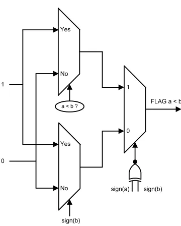
5.1.1 Flag Generator Module . . . 49
5.1.2 Lower Bound and Upper Bound modules . . . 55
5.1.3 Scale Synchronizer module . . . 66
5.1.4 Scale L and Scale U modules . . . 77
5.2 Pipelined Architecture of the Design . . . 79
5.2.1 Need for Pipelining . . . 79
5.2.2 Architectural Issues with Pipelined Designs . . . 81
5.2.3 Superpipelining for High Throughput . . . 87
6 Testing and Results 90 6.1 Simulation Results . . . 90
6.1.1 Interval mode of operation . . . 91
6.1.2 Pointwise mode of operation . . . 93
6.2 Synthesis Results . . . 95
6.2.1 The Non-pipelined Architecture . . . 96
6.2.2 Synthesis of Pipelined Designs . . . 96
6.3 Power Analysis . . . 99
7 Architectural Insights 103 7.1 Throughput for the BFPIALU . . . 103
7.1.1 The Probability of Overflow in the BFPIALU . . . 103
7.1.2 Evaluating Throughput for the BFPIALU . . . 104
7.1.3 Type-1: MAC operations in Pipelined Designs . . . 106
7.1.4 Type-2 : Non-MAC operations in Pipelined Designs . . . 111
7.2 Structural Hazards . . . 113
7.2.1 Dual MAC structure for pointwise computations . . . 114
7.3 Error Analysis . . . 117
7.3.1 The Input Data Sequence . . . 118
7.3.2 Input Scaling Error Analysis . . . 118
7.3.3 CBFS Error Analysis . . . 120
8 Conclusion and Future Work 124
8.1 Conclusion . . . 124
8.2 Future Work . . . 127
8.2.1 Short Term Goals . . . 127
8.2.2 Long Term Goals . . . 127
List of Figures
1.1 Wrap around in two’s complement arithmetic. . . 3
1.2 Wrap around in divergent interval series (Q7.8 format) . . . 5
3.1 Dividing data into blocks . . . 18
3.2 Hardware environment for the BFPIALU . . . 23
3.3 Interval BFP system with CBFS . . . 29
4.1 Two’s complement Q0.15 fixed point representation . . . 33
4.2 Capturing bit growth . . . 38
5.1 Top Level Block Diagram . . . 46
5.2 Flag Generation Module . . . 51
5.3 Disjoint intervals X and Y . . . 53
5.4 Comparison Unit to compare two Q0.15 numbers . . . 54
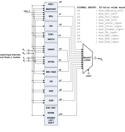
5.5 Command, MAC and maxexpsignal Select logic . . . 55
5.6 Lower Bound Module . . . 57
5.7 Multiplexed Addition and Midpoint operation . . . 58
5.8 Multiplexed Subtraction and Width operation . . . 58
5.9 Hardware for Multiplication in Lower Bound module . . . 59
5.10 Multiply-Accumulation scheme in hardware . . . 60
5.11 Hardware for overflow detection . . . 61
5.12 Logic for interval Union and Intersection in Lower Bound module . . 62
5.13 Logic for Min and Max commands in Lower Bound module . . . 62
5.14 Logical XOR operation . . . 63
5.15 Exponent Detection scheme . . . 64
5.16 Normalization scheme . . . 65
5.17 Top Level View of the Scale Synchronizer module . . . 66
5.18 Hardware module to Handle the Special Case of Rounding . . . 70
5.19 Scaling Modules for Iterative Computations . . . 78
5.21 Combinational Multiplier . . . 81
5.22 Three Stage Pipelined Multiplier . . . 81
5.23 Five Stage Pipelined Multiplier . . . 81
5.24 Collision Analysis for the Partially Pipelined BFPIALU . . . 82
5.25 Collision Analysis for the Fully Pipelined BFPIALU . . . 83
5.26 Scheme 1 : Multiply-Add pipeline . . . 84
5.27 Scheme 2 : Multiply-Add pipeline . . . 85
5.28 Scheme 2 : Post-Overflow Multiply-Add pipeline . . . 86
5.29 Critical path and Architecture of the Three stage Pipelined Design . 88 5.30 Critical path and Architecture of the Highly-Pipelined Design . . . . 89
6.1 Simulation results for BFP commands (interval mode) . . . 91
6.2 Simulation results for Min, Max, OR, AND, XOR (interval mode) . 92 6.3 Iteration of Summing a Series with Overflow (interval mode) . . . . 93
6.4 Independent pointwise operation in the interval ALU . . . 94
6.5 CBFS in an iteration with overflow in the Upper Bound. . . 94
6.6 Special case of Rounding in the pointwise¯ mode . . . 95
6.7 Area distribution between Modules . . . 97
6.8 Timing report for Superpipelined designs . . . 98
6.9 Area report for Superpipelined designs . . . 98
6.10 Code Segment to Generate Random Intervals . . . 101
6.11 Power Dissipation for the Superpipelined designs with 1000 vectors . 102 7.1 Example to illustrate MAC computations with N=6 and k=4 . . . . 107
7.2 Post-overflow Corrective Actions . . . 108
7.3 Illustration of MAC computations with one overflow for N=6 and k=4 109 7.4 Post-overflow Corrective Actions : MAC pipelines with single delay . 110 7.5 Throughput Across Pipelined Designs . . . 112
7.6 Difference Equation for an FIR filter . . . 115
7.7 Feeding inputs to the Dual MAC structure for an FIR Filter . . . 116
7.8 Input sequence for Error analysis . . . 119
7.9 Filtered output : Input scaling vs CBFS . . . 122
List of Tables
2.1 9 cases of interval multiplication . . . 12
2.2 Interval Division A/B with A,B ∈ <, 0 ∈ B . . . 13
2.3 Interval Division A/B with A,B ∈ <, 0 not in B . . . 13
3.1 Exponent Detection in a data block of size 4 . . . 19
3.2 Grouped Output Points Sharing a Common Exponent. . . 30
4.1 Dynamic Range/Precision chart for 16-bit Q-formats . . . 32
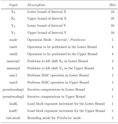
5.1 Architecture Input Description. . . 48
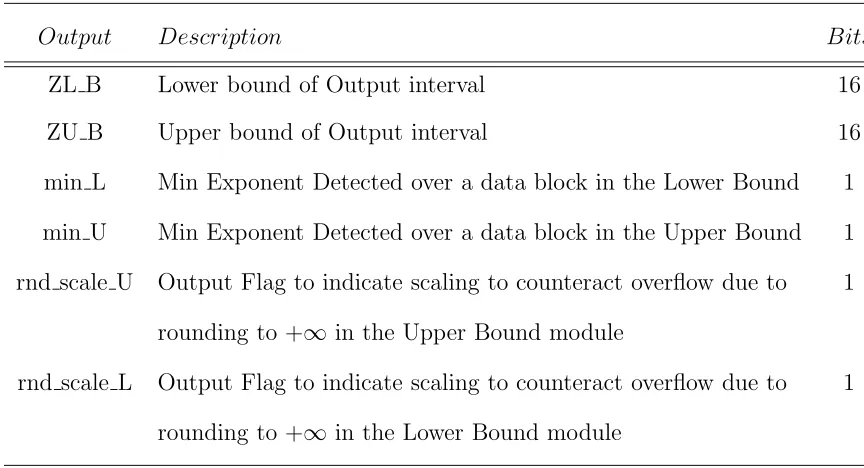
5.2 Architecture Output Description. . . 49
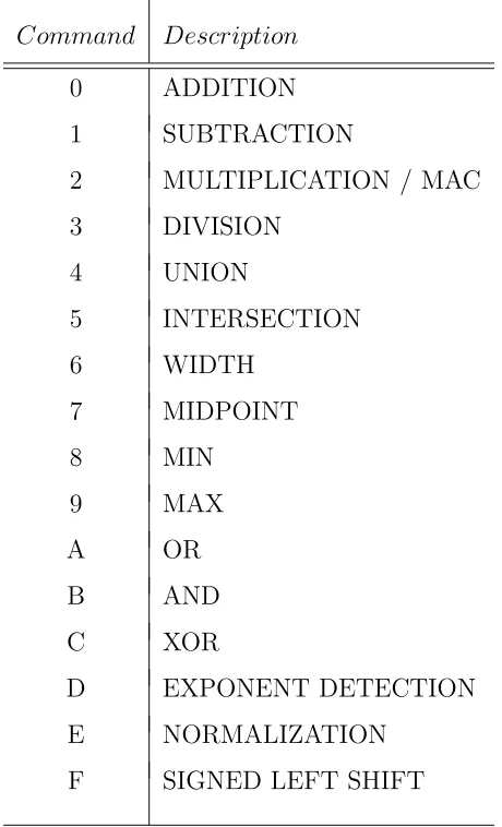
5.3 Command Set for the ALU. . . 50
5.4 The Scheme of Flags . . . 51
5.5 Deriving mul from the Flags . . . 52
5.6 mul signal for the different cases of interval multiplication . . . 52
5.7 Priority Encoder array for Exponent Detection . . . 65
5.8 Scale Synchronization for Interval Operations . . . 73
5.9 Scale Synchronization for Lower Bound module : Truncation . . . 74
5.10 Scale Synchronization for Upper Bound module : Truncation . . . 74
5.11 Scale Synchronization for Lower Bound module : Rounding to +∞ . 75 5.12 Scale Synchronization for Upper Bound module : Rounding to +∞ . 76 6.1 Timing for Non-pipelined Design . . . 96
6.2 Area and Timing Report for different Superpipelined designs . . . 99
6.3 Area and Timing Report for the Highly-Pipelined Design . . . 99
6.4 Power Dissipation for Pipelined Designs with 1000 input vectors . . . 101
7.1 Commands Function Table (Point-wise Operations) . . . 114
7.2 Error with Input Scaling . . . 120
7.3 Error with CBFS . . . 121
Chapter 1
Introduction
Modern numerical analysis with real numbers includes the techniques of interval analysis andtheoreticalanalysis [1]. Interval analysis performs arithmetic onrangesof real numbers known as intervals, whereas theoretical analysis performs arithmetic on
exactreal numbers. Today, interval analysis is a mature discipline and finds use in not only digital signal processing applications such as fuzzy adaptive filtering [2] and error
analysis [1] but also control applications such as decision systems [3].
Knowledge-based systems employ intervals to model imprecise quantities such as knowledge [4].
Many interval-based algorithms have been developed to address more and more com-plex problems such as solving systems of nonlinear equations, determining eigenvalues
and eigenvectors of matrices, finding roots of functions, and performing global
opti-mization [5].
Recognizing the growing importance of interval-based algorithms, software pack-ages such as the Sun Forte Fortran 95 compiler, the GNU Fortran compiler, the Sun
C / C++ compiler, Frink programming language, Boost C++ package and many
others provide support for interval arithmetic. The complete list of software that
per-formance [7]. The cause for this is attributed to the overhead due to function calls,
memory management issues, error and range checking, changing rounding modes,
ex-ception handling and many others [8]. Furthermore, checking the sign of the input interval endpoints for interval multiplication leads to a set of conditional statements.
This, in turn, could lead to frequent flushing of pipelines in a processor. These issues
are computationally costly and can be mitigated by providing hardware support for interval operations.
Gupte, R. et.al. [9] implemented a fixed point Arithmetic Logic Unit (ALU) ded-icated to interval computations for digital signal processing and control applications
to address the problem of slow program execution. While the interval ALU is
compet-itive in its throughput and power consumption, it is prone tooverflow errorsowing to bit growth beyond the limits of the fixed point numeric representation. Overflow can
occur when frequently used operations such as multiply-accumulate are performed
successively a large number of times in this implementation. Interval arithmetic can cease to be reliable and this defeats the main purpose of using it. Interval arithmetic
aims to provide reliable bounds on the results of point-wise evaluations, thereby
pro-viding a certificate of reliability to such computations.
This work explores the Block Floating Point (BFP) hardware scheme with
condi-tional output scaling to handle overflow errors and provide reliable interval arithmetic. Superpipelining is applied to the basic architecture to obtain designs with a higher degree of pipelining. The result is a set of designs that can operate at higher clock
rates. The choice of the optimal design from this design space is performed by
pri-oritizing throughput based on factors such as clock rate, number of overflows and the number of pipeline stages for the intended application. Throughput is a very
1.1
Description of the Problem
Fixed point implementations in hardware are found to be small in size, involve low implementation costs and have low power consumption as compared to their floating
point counterparts when all factors such as the number of bits are kept identical. In
spite of these advantages, fixed point designs are plagued by the problem of small
dynamic range. A limited dynamic range leads to overflow errors when we represent binary numbers whose bit length exceeds the limits imposed by the chosen number
format. In the normal overflow scheme for fixed point two’s complement arithmetic,
overflow results in wrap-around, where attempts to represent a positive number just outside the representable range results in its interpretation as a large negative number,
and vice versa [10]. The consequence is that the computed result no longer represents
the true value and this makes wrap around a highly undesirable phenomenon.
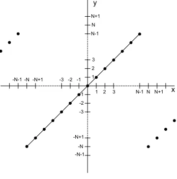
Figure 1.1 depicts the case for overflow in two’s complement fixed point integer arithmetic with a maximum value of +(N-1)and a minimum value of -N, where N is the limit for number representation with a finite number of bits.
Figure 1.1: Wrap around in two’s complement arithmetic.
interval arithmetic. By definition, a closed finite real interval is defined as an
or-dered set of all real numbers {x ∈ < : a≤x≤b} lying between and including the real endpoints a and b. Closed in this particular context means the endpoints are included as a part of the interval. Therefore, an interval represents a range of real
numbers bounded and denoted by its endpoints. Interval operations are performed
on the interval endpoints which are represented using fixed point or floating point in computer arithmetic. We present an example that clearly illustrates the outcome of
wrap around in the Q7.8 fixed point format, devoting 8 bits to integer representation
and 8 bits to the fractional part. By doing this, we aim to highlight the overflow errors that beset the work of [9].
We choose the Q7.8 format in order to match the input data format of the interval ALU of [9]. The interval ALU stored its intermediate interval endpoints in the 32-bit
Q15.16 fixed point format and a 16-bit integer output was obtained by performing
outward rounding on the fractional part of both interval endpoints. In this
experi-ment, we compute the sum of an interval divergent geometric series
N X
n=0
an with a =
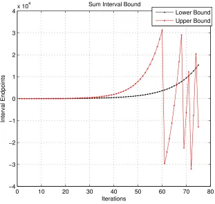
[1.10, 1.15] and N arbitrarily equal to 75 as if it were computed in the interval ALU. Such a computation enables us to observe the fast growth in the magnitude of the
terms and wrap around can be observed better.
It is observed that when the magnitude of the upper bound exceeds +32767, it
wraps around the positive maximum and assumes a value which is less than the lower bound. Therefore, the result is incorrect and a state of error has been entered since
the output interval does not enclose the true result. Figure1.2illustrates the incorrect output intervals obtained after overflow.
The above mentioned experiment clearly indicates that an appropriate scheme is
needed so that the integrity of interval computations is maintained. We feel the need for firm guidelines to formulate such a scheme and ensure that fixed point interval
0 10 20 30 40 50 60 70 80 −4
−3 −2 −1 0 1 2 3 4x 10
4 Sum Interval Bound
Iterations
Interval Endpoints
Lower Bound Upper Bound
Figure 1.2: Wrap around in divergent interval series (Q7.8 format)
expand the capabilities of the interval ALU [9] so that exact or point-wise evaluations
may also be performed in the interval ALU and both theoretical and interval analysis
can be performed in the same ALU efficiently. All these factors have led to the development of an interval ALU with Block Floating Point support.
1.2
Background
With the increasing importance of fast execution for interval-based algorithms, the focus has shifted to the development of competitive interval hardware
architec-tures that match the performance of non-interval architecarchitec-tures. While floating point
as a solution to poor execution rates, there is only one dedicated fixed point interval
ALU for DSP and Control applications that has been designed and tested [9]. The
fixed point interval ALU has dedicated modules for computing the upper and lower bounds of the interval output and is followed by a dedicated rounding module that
performs outward rounding on the interval result. This design has recorded a com-petitive throughput on the order of 56 MIOPS (Millions of Interval Operations per Second) for the non-pipelined design and about 307 MIOPS for a 7-stage pipelined
design [9]. A shortcoming of the design is that overflow errors are not taken into
con-sideration. Therefore, the accumulator overflows over a large time of accumulation leading to unreliable results. The proposed interval ALU, developed in this work,
utilizes the skeleton of its architecture from the design of [9].
The proposed interval hardware will adhere strictly to certaincriteria for reliable results. The work of Van Emden [14] established these criteria ascorrectness, totality, closedness, optimality and efficiency for floating point interval arithmetic. These same criteria have been adopted for the fixed point implementation since the Block Floating Point (BFP) operations using the proposed interval ALU are performed on
the underlying fixed point hardware. These criteria serve as a guideline for making critical decisions pertaining to the hardware design such as the selection of appropriate
rounding modes and overflow handling techniques.
Our work explores the architecture of a BFP arithmetic-based interval ALU in
order to provide reliable interval operations. BFP arithmetic provides a dynamic
range higher than that provided by conventional fixed point representations. In a
typical BFP implementation, the input data is divided into non-overlapping blocks along with an integer block exponent term associated with each block. It is possible
to detect the magnitudes of data samples in a block of data and then normalize them to bring them all to a common exponent so that fixed point computations may
be performed. BFP arithmetic support for point-wise evaluations in most DSPs is
redundant sign bits present, thereby indicating its magnitude [16]. A small number
of redundant sign bits indicates a large magnitude for the sample, and vice versa.
Exponent Detection is performed over a block of data to identify the largest magnitude among all samples and then all the data samples in that block are shifted left by this
number. Hence, all data samples in that block are normalized and carry the same
exponent. Therefore, fixed point computations can be performed. Normalization implies Exponent Detection followed by left shifting in a single operation [15]. BFP
arithmetic has been successfully applied to digital filters [17] and the Fast Fourier
Transform [15] [18].
Most commercial DSPs today support BFP operations for point-wise
evalua-tions. Fixed point DSPs such as Analog Devices ASDP-21xx, Texas Instruments TMS320C54x [15], SGS-Thomson D950-CORE, Zoran ZR3800x, DSP Group
OakD-SPCore and uPD7701x provide single cycle Exponent Detection. However, DSPs
from the AT&T DSP16xx family (other than DSP1602 and DSP1605) are the only ones that provide single cycle Normalize instructions. Other DSPs such as the Texas
Instruments TMS320C2x, TMS320C5x, the DSP Group PineDSPCore, the Motorola
DSP5600x and DSP561xx provide iterative normalization instructions where an n-bit number takes n-cycles to normalize [15]. However, these DSPs do not provide
spe-cialized interval arithmetic support with BFP, which is necessary while considering
the issues of reliability.
The information on BFP arithmetic is not complete without a mention of the
techniques that are used handle overflow errors. The choice of a good overflow
han-dling scheme that also meets the criteria mentioned above is essential to perform reliable fixed point interval arithmetic. The overflow handling techniques are named
1.3
Contribution
This thesis makes the following contributions to the current work on fixed point interval hardware architectures. To the best of our knowledge, no other current
research has applied the concept of BFP arithmetic to intervals in order to achieve
reliable arithmetic.
1. We present an interval ALU with BFP arithmetic support and CBFS for
han-dling overflow errors in fixed point operations
2. We modify the interval architecture to facilitate both point-wise operations for theoretical analysis and interval operations for interval analysis
3. We expand the command set for the interval ALU by introducing logical and
comparison operations
1.4
Thesis Organization
This thesis is organized in the following manner: Chapter 2 introduces interval
arithmetic and describes its operations. It also describes the criteria that serve as a guideline to implement reliable arithmetic in fixed point hardware. Chapter 3
discusses Block Floating Point arithmetic. It describes two overflow handling
tech-niques associated with BFP arithmetic, namely Input Scaling and Conditional Block Floating-point Scaling (CBFS). Chapter 4 presents the Q0.15 fixed point format and
illustrates how to perform fixed point arithmetic, logical, comparison and Block
Float-ing Point operations in this format. Chapter 5 describes the hardware architecture for the interval ALU with detailed module descriptions. It also describes superpipelining
as a means of achieving higher throughput. Chapter 6 presents the results of
simula-tion, synthesis and power analysis for the hardware architecture of the BFP interval
ALU. Chapter 7 discusses the evaluation of throughput for the BFP interval ALU as a function of the number of overflows, number of pipelined stages and the fastest
performing point-wise computations in the architecture. This chapter also describes
an experiment to perform error analysis on Input Scaling and CBFS to identify the
Chapter 2
Reliable Interval Arithmetic
Real numbers are of infinite precision while digital machines can only provide limited accuracy on them. By definition, a computer represented set of real numbers
M is a quantized encoding of the elements of a set of real numbers<. The aim of an
optimal computer representation is to maximize the number of elements mapped from
< on to M [22] given a restricted number of bits for data representation. Floating
point and fixed point representations form two widely used discrete approximations
to<.
Interval arithmetic acknowledges limited precision in computer representation [14]
and provides bounds on the error accrued from computations involving discrete ap-proximations. For this reason, it is important that computer arithmetic involving
intervals should stay reliable at all times and should not fall into a state of error due
to the limitations of number representation in the computer. This chapter discusses the basic interval and set operations followed by a description of a set of criteria that
2.1
Interval and Set Operations
The basic interval and set operations include addition, subtraction, multiplication, division, union, intersection, width and midpoint. These operations are important for
many applications in signal processing, one example of which is global minimization
of cost functions for adaptive IIR filtering [23]. These operations are described below
for intervals I = [r,s] and J = [u,v].
A. Interval Addition
I +J = [ r +u,s + v ]
Interval addition involves adding up the corresponding end-points for the input
interval arguments. Therefore, the lower end-point for the output interval is the sum
of the lower end-points of the input intervals while the upper end-point for the output interval is the sum of the upper endpoints of the input intervals. For example, [1,2]
+ [4,6] = [5,8]
B. Interval Subtraction
I- J = [ r -v,s - u ]
Interval subtraction involves subtracting the upper endpoint of the second inter-val from the lower endpoint of the first interinter-val to obtain the lower endpoint for the
output interval. Similarly, a subtraction of the lower endpoint of the second interval
from the upper endpoint of the first interval yields the upper endpoint for the output
interval. For example, [3,4] - [1,2] = [1,3]
C. Interval Multiplication
I *J = [ min (ru, rv, su, sv), max (ru, rv, su, sv) ]
This operation can be reduced to a set of conditional operations based upon the
signs of the endpoints of the input interval arguments. There are nine possible cases
Table 2.1: 9 cases of interval multiplication
Case Description Output Interval Bounds
1 xL ≥ 0;yL ≥ 0; [xLyL,xUyU]
2 xL ≥ 0; yL < 0 ≤ yU; [xUyL,xUyU]
3 xL ≥ 0; yU < 0; [xUyL,xLyU]
4 xL < 0 ≤ xU; yL ≥ 0; [xLyU,xUyU]
5 xL <0 ≤ xU;yU < 0; [xUyL,xLyL]
6 xU < 0; yL ≥ 0; [xLyU,xUyL]
7 xU <0; yL < 0 ≤ yU; [xLyU,xLyL]
8 xU < 0;yU < 0; [xUyU,xLyL]
9 xL < 0 ≤ xU; yL < 0 ≤ yU; [min( xUyL,xLyU), max(xLyL,xUyU)]
An example is [1,4] * [2,3] = [2,12] which is a case where none of the input intervals enclose a zero.
D. Interval Division
Interval Division involves eight cases depending upon whether a zero is contained
in the denominator interval or not. The general algorithm used to perform this
operation is presented in Table2.2and Table2.3[7]. It can be implemented similar to multiplication using a set of flags to indicate the choice of operands used in the division
operation. However, most DSPs do not provide the divide instruction because this
operation occurs very infrequently in signal processing applications. Alternatively, dividing by powers of 2 reduces the operation of division to right shifting operations
Table 2.2: Interval Division A/B with A,B ∈ <, 0∈ B
Case A = [xL,xU] B = [yL,yU] A/B
1 0 ∈ A 0 ∈ A (-∞,∞)
2 0 ∈/ A B = [0,0] []
3 xU < 0 yL <yU = 0 [-xU/yL,+∞)
4 xU < 0 yL <0 <yU (-∞, xU /yU] ∪[xU /yL, +∞)
5 xU < 0 0 = yL <yU (-∞, xU/yU)
6 xL >0 yL <yU = 0 (-∞, xL/yL,)
7 xL >0 yL <0 <yU (-∞, xL /yL]∪ [xL /yU, +∞)
8 xL >0 [0 = yL < yU [xL /yU, +∞)
Table 2.3: Interval Division A/B with A,B ∈ <, 0 not in B
Case A = [xL,xU] B = [yL,yU]
xU <0 [xL /yL, xU /yU] [xU /yL, xL /yU]
xL <0 <xU [xL /yL, xU /yL] [xU /yU, xL /yU]
xL > 0 [xL /yU, xU /yL] [xU /yU, xL /yL]
E. Interval Union
Given that I and J are not disjoint, interval union is denoted by
I ∪J = [min(r, u), max(s, v)]
For example, given I = [2, 4] and J = [3, 6] yields I ∪ J = [2, 6]. This operation is expensive for the case when the sets are disjoint. Throughput is affected if the
F. Interval Intersection
Given that I and J are not disjoint, interval intersection is denoted by
I ∩J = [max(r, u), min(s, v)]
A null set results if the input intervals are disjoint and do not contain any real
num-ber elements in common. In this case, the ALU sets a disjoint flag at the end of the operation to indicate disjoint inputs. For example, [1,5] ∩ [4,8] = [4,5]
G. Interval Width
W(I) = s-r
This operation is performed on a single interval. In the case of the interval I, the width W is given by the difference of the upper bound and the lower bounds.
H. Interval Midpoint
This operation is also performed on a single interval. The midpoint M for the interval I is given by
M(I) = (r + s)/2
I. Additional Operations
The command set for the interval ALU developed in this work also includes
logi-cal, comparison and Block Floating Point (BFP) operations. Logical operations such as bitwise-AND, bitwise-OR and bitwise-XOR have been added from the perspective
of a computation engine that performs point-wise operations. Logical operations in
DSPs are used widely in applications such as error control coding [24]. The logical operations in the interval ALU operate on the upper and lower bounds for an interval
argument. Thus, for interval I, these operations are performed as (s ∨ r), (s ∧ r) and (s ⊕ r) for OR, AND and XOR operations respectively. Comparison operations
of two intervals are used to evaluate their minimum and maximum values simultane-ously. Applications such as fuzzy adaptive filters based on interval Type-2 systems
require such computations [2]. Therefore, for intervals I and J mentioned above, the operations is performed as follows:
min(I,J) = [min(r,u), min(s,v)]
The command set also contains Block Floating Point operations. These are, however,
described later in Section 3.1.2 and 4.4.2.
It has been demonstrated in Section 1.1 that overflow can lead to unreliable
in-terval arithmetic. Overflow occurs when the result of an operation requires more bits
on the MSB side for true representation than what is available in the machine [25]. Overflow results primarily from the operations of addition and subtraction. Overflow
can also occur with the accumulation of products after multiplication. The cause of
overflow is traced to the operation of addition in this case. Having introduced the operations to be performed in the interval ALU, we next discuss the criteria, which
when met, leads to reliable interval arithmetic.
2.2
Criteria for Reliable Interval Arithmetic
Van Emden [14] has proposed correctness, closedness, totality, optimality and
ef-ficiency for the criteria in evaluating interval hardware. We consider a fixed point
Interval arithmetic system, based on setting the interval endpoints to finite values, that abides by this set of criteria summarized below:
A. Correctness
An interval operation is said to becorrectwhen it yields an output interval contain-ing all the results of point-wise evaluations based on point values which are elements
of the argument intervals. For example, if X = [1,2] and Y = [3,5], then this criterion applied to the addition operation (+) implies that the resultant interval [4,7] must contain the results of all point-wise additions (x+y) with x ∈ X and y ∈ Y.
B. Totality
A total interval operation is one that is defined for all possible input arguments. For example, designers face a problem with defining the operation of division (/) when
the operation of division by excluding 0 from the denominator.
C. Closedness
A closed interval operation on the set of real numbers < is one that operates on intervals whose endpoints are in<and yields an output interval whose endpoints are
also in <. For example, if the operation is multiplication and the input arguments are [1,2] and [3,4], then the result of this operation is [3,8]. Since this operation
re-sults in an output interval whose endpoints are real values, we can say that interval
multiplication is closed on the set of reals.
D. Optimality
This criterion ensures that the operation is not performing any overestimation and
that the bounds are the most optimized ones for the type of representation chosen. The arithmetic should be such that the resultant interval is not wider than necessary.
This is applicable to operations such as addition, subtraction, multiplication and
di-vision.
E. Efficiency
Efficiency is defined with respect to the implementation of the interval arithmetic in hardware. One way to measure efficiency is through the execution speed which
can be improved by eliminating subroutine calls in software or by providing special
purpose hardware that deals with the same operation in a much faster way. Efficiency can also be measured in terms of power dissipation or throughput.
It is absolutely essential that arithmetic in the chosen computer representation adheres to the criteria mentioned above for reliable interval computations. The
Chapter 3
Block Floating Point Arithmetic
Block Floating Point (BFP) is a scaled number representation format similar to floating-point, but its arithmetic operations are performed in fixed point. BFP
arith-metic provides a useful tradeoff between the large dynamic-range with the increased
hardware complexities of floating point implementations and the limited dynamic range with the relative simplicity of fixed point implementations [26]. Applications
for signal processing such as digital filters, calculation of the Fast Fourier Transform
and Fast Hartley Transform utilize BFP arithmetic [19].
3.1
Block Floating Point Representation
BFP representation can be considered to be a special case of floating point
repre-sentation where a block of N numbers has a joint scaling factor corresponding to the
maximum magnitude of the numbers in the block. Ifxi represents theithdata sample
and γ represents the block exponent, then the BFP representation is denoted as
[x1, x2, ..., xN] = [ˆx1, xˆ2, ..., xˆN ]·2γ where ˆxi = xi · 2−γ
The block exponent γ is defined by
where M = max(|x1|, ... ,|xN|), b.c is the floor function and |xˆi| ∈[0,1]. The integer
S signifies a constant scaling term for the block exponent which is needed in certain
applications like filtering [19].
3.1.1
Data Representation
Data stored in the memory is grouped into non-overlapping blocks of ‘N’
consec-utive samples to perform BFP arithmetic. Each block of data is separately quantized
for BFP representation and processed. Figure 3.1 shows the division of an arbitrary data sequence into blocks of size 700.
3000 3500 4000 4500 5000
-0.6 -0.4 -0.2 0 0.2 0.4 0.6
Figure 3.1: Dividing data into blocks
Data processing in BFP arithmetic is performed on a block basis. Within a
particular block, all data samples are associated with one common exponent term.
From the definition of BFP representation, it is evident that the block exponent γ
can be computed from the values of M and S. The use of S is optional and based upon
is known as Exponent Detection, and the operation of scaling all the data samples in
the data block by 2−γ is known as Normalization. Samples in a data block may be
distributed over a wide range of values. Normalizing a data block brings all samples in the data block to a common exponent value and enables fixed point operations to
be performed on the samples. It is evident that Exponent Detection and Left shifting
by γ boosts the strength of the input data.
3.1.2
Normalization of a data block
Table 3.1 illustrates how to identify the value ofγ for a block data size of 4. The data samples are represented in the decimalnumber system and S is fixed at 0. We assume that the dynamic range is [-1,1] and that all data samples are fixed point
values which share a pre-normalization common exponent value ‘C’. The updated
block exponent after normalization will be (C +γ).
Table 3.1: Exponent Detection in a data block of size 4
Data Samples (x) N ormalized Data(ˆx) γ = (blog10 Mc + 1)
0.189 0.189
0.214 0.214
M = 0.333
-0.265 -0.265
γ = 0
0.333 0.333
0.087 -0.870
-0.096 0.960
M = 0.096
-0.0014 -0.014
γ = -1
In each data block, the sample with the largest magnitude is chosen to compute
the block exponent γ. Therefore, M = 0.333 for the first data block and M = 0.096
for the second block. The value of γ post-normalization is equal to (C) and (C-1) for the first and second data blocks, respectively.
A more intuitive approach to compute the value of γ for samples represented in the decimal system is to assign it with the negated count of the leading zeros for the
sample with the largest magnitude in a data block. In the first data block, M = 0.333
does not bear a leading zero digit and hence γ = 0. For the second data block, M = 0.096 bears one leading 0 and hence γ = -1. This scheme can be extended to the
binary system where each sample is represented in two’s complementary fixed point
representation. Here, data samples of small magnitude are fit to the available word size by sign extension. The block exponent γ is assigned the least value of leading
redundant sign bits obtained by traversing through all the samples in the data block.
Evidently, this value will correspond to the sample with the largest magnitude in the data block. The procedure to normalize the data entails left shifting of all data
samples in the entire block of data by γ positions to bring them all to a common
exponent value. Henceforth, fixed point operations can be carried out on data samples from this block.
We now present an example that illustrates block normalization for samples repre-sented in two’s complement fixed point arithmetic. Consider the example for a block
of data comprised of four samples 0.0000100, 0.0011000, 0.0000001 and 0.0001111 in
the Q0.7 format. The value of M is identified to be 0.0011000 because it has the least
number of leading sign bits. The value of γ is identified to be (-2). Hence, every sample in that data block is left-shifted by two places to bring all samples to a
com-mon exponent. Therefore, the data samples bear the values of 0.0010000, 0.1100000, 0.0000100 and 0.0111100 and the number of shifts is (00000010) for an 8-bit
expo-nent. The updated block exponent will be (C-2). The same procedure is applicable
3.1.3
Normalizing an interval data block
Every interval is represented by two endpoints and therefore, two data memory banks must be considered while implementing it in hardware. In this work, we
inves-tigate the scenario where normalization is performed such that both endpoints of all
intervals in an interval block of data share the same block exponent. Therefore, fixed point operations can be performed on the data directly.
The definition of BFP representation presented in Section 3.1 is extended for
interval data. If [xLi, xU i] represents the ith interval data sample and γ represents the
interval block exponent, then the BFP representation is denoted as
[ [xL1,xU1], [xL2,xU2], ..., [xLN,xU N ] ] = [ [ˆxL1,xˆU1], [ˆxL2,xˆU2], ..., [ˆxLN,ˆxU N] ]·2γ
where [ˆxLi,ˆxU i] = [xLi,xU i] · 2−γ
The block exponent γ is defined by
γ =b log2 M c+ 1 + S
where M = max(|xL1|, |xU1|, ...,|xLN|, |xU N|) and |xˆLi| ∈ [0,1]; |xˆU i| ∈ [0,1]. The
integer S signifies a constant scaling term for the block exponent and will effect both
endpoints in a similar way.
The procedure to identify the block exponent,γ, for a data block comprised of interval
data is described next. It is divided into three steps:
1. Identify the minimum number of redundant sign bits among the point-wise
data comprised of both endpoints of all the intervals in the block. This helps
to identify the largest magnitude-valued endpoint in the interval block.
2. Left-shift both endpoints of every interval in this block by this number.
3. If ‘C’ was the common block exponent pre-normalization, update the block
exponent to a value (C+γ). Store the block exponent in a single location for the interval data block for future reference.
We detect that among these four endpoints, the minimum number of redundant sign
bits is present in 0.0010000 and is equal to 2. Therefore, all endpoints are left shifted
by 2 positions and the intervals are normalized to the same exponent. Therefore, the normalized intervals are [0.0011000, 0.1000000] and [0.0110100, 0.0111100]. The
block exponent for this interval data block is decremented by 2 as compared to the
previous exponent.
3.1.4
BFP Hardware Environment
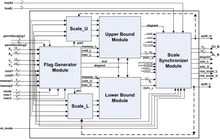
The Block Floating Point Interval Arithmetic and Logic Unit (BFPIALU)
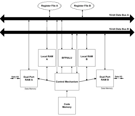
devel-oped in this work is intended to be housed in an interval processor with the capability to perform BFP operations. A rough sketch of the environment surrounding the
BF-PIALU is shown in Figure 3.2.
The data buses for this system are 16-bit bidirectional lines, labeled Data Bus
A and Data Bus B, dedicated to the lower and upper endpoints of the interval data
respectively. The instructions to be executed are stored in the Code Memory. The Dual Port RAMs labeled A and B comprise the system data memory which are used
to store the lower and upper interval data endpoints respectively. They receive data
from system I/O data transfers. The Local RAMs, labeled A and B, constitute the local storage for working interval data. These could be useful, for instance, to
store the data interval blocks between Exponent Detection and Normalization since
the complete procedure requires two traversals through the same data block. The underlying assumption is that Local RAMs are much faster than the Dual Port RAMs.
The BFPIALU is the key data processing element in this architecture. It performs
arithmetic, logical and BFP operations in fixed point. The Register Files are used for temporary data storage, such as intermediate results from the BFPIALU. They
are comprised of a set of high-speed data buffers dedicated to the lower and upper
! "
Figure 3.2: Hardware environment for the BFPIALU
• It takes care of fetching instructions from the code memory, decoding them and transferring the data to the appropriate destination.
• It interacts with the Dual Port RAMs and Local RAMs for reading and writing data. It also generates addresses for these operations.
• It feeds the data, applies the necessary command and associated control signals
for the BFPIALU.
• Optionally, it houses a DMA mechanism to handle memory interactions
involv-ing large amounts of data.
The hardware environment for the BFPIALU may be changed at a later stage suitably to match the requirements of the processor designer. However, care must be
taken to ensure that the data feed mechanism and control signals to the BFPIALU
remain unchanged.
3.2
Overflow Handling Techniques
Reliability becomes a very significant issue when interval operations are performed
in the BFPIALU. The arithmetic performed should be able to cope with and not fall
prey to the errors caused by bit growth on the MSB side of the result. Fixed point
implementations especially have to deal with overflow errors owing to the availability of a small dynamic range. Since BFP arithmetic is performed in fixed point, additional
care must be taken to avoid overflow in BFP arithmetic by adopting appropriate
techniques that can either prevent or correct overflow errors.
This work investigates the techniques of pre-operation input data scaling (or a priori scaling) and post-operation output data scaling (or a posteriori scaling) for a given fixed point operation. The former is known as Input Scaling, whereas the latter
is known as Conditional Block Floating-point Scaling (CBFS). A brief description of
each of these techniques is presented next.
3.2.1
Input Scaling
The technique of Input Scaling is based on the priciple ofpreventingthe occurence of overflow errors. From the definition of BFP provided in Section 3.1, Input Scaling
entails a scaling of the input data block using a constant scaling factor ‘S’ while normalizing it. The value of S is chosen depending upon the number of operations to
so that fixed point additions can freely be performed on the scaled data without any
concern of overflow during the actual operation. Input Scaling is fast and simple.
All data samples in an output block share the same block exponent, which is equal to the block exponent of the normalized input. This technique is compared to the
Conditional Block Floating point Scaling (CBFS) scheme which is discussed next.
3.2.2
Conditional Block Floating-point Scaling
This technique is based upon the idea of correcting overflow errors. The output block exponent is determined a posteriori without using the constant integer scaling term ‘S’ during normalization. After normalization, the data samples are brought into the fixed point hardware for computations. If no overflow occurs, then the output
block exponent is kept the same as the normalized input block exponent. However,
if overflow occurs, then a set of corrective actions are taken. These are listed below:
1. The hardware block scales the erroneous output down by a factor of 2. This is
performed by right shifting the result of the operation in fixed point.
2. The output block exponent is updated to the incremented value of the input block exponent and the result is stored.
3. If the computations are iterative in nature and an intermediate overflow occurs,
then all inputs from that point onwards are scaled down by an additional factor of 2. This process is repeated at each instance of overflow.
We next present a listing of the major differences between the techniques of Input
Scaling and CBFS:
1. CONSTANT SCALING FACTOR ‘S’
Input Scaling uses a preset constant scaling factor S in anticipation of overflow
during normalization. For evaluating dot products, the value of ‘S’ can be chosen depending upon the number of additions to be performed on the data.
CBFS implementations do not scale the input data during normalization and
set S = 0. Under this scheme, the operation is first performed and the output
is scaled down by a factor of two only in the event of overflow.
2. OVERFLOW DETECTION CIRCUITRY
Since Input Scaling is centered on the idea of preventing overflow errors by pre-scaling of inputs, no overflow detection circuitry is required. CBFS imple-mentations are based on the idea ofcorrectingoverflow errors and hence involve overflow detection circuitry.
3. OUTPUT BLOCK EXPONENT
The exponent for the output of individual operations such as addition and
sub-traction for Input scaling is the same as that of the normalized input data. For
CBFS implementations that run long iterative operations such as computation of dot products, the output block exponent will change depending upon whether
overflow occured or not. Thus, normalizing the output data could consume more
time leading to slower implementations.
4. ACCURACY
Input Scaling implementations record poor accuracy because they scale the
in-put data down unconditionally by a pre-determined factor ‘S’ before performing the operations. Therefore, such implementations assume the worst-case scenario
for every operation - that overflow will occur after every addition. This
uncon-ditional scaling lowers accuracy. In contrast, CBFS implementations scale input data by half from the point that overflow actually occurs. The output is scaled
only if overflow occurs. This need-based scaling approach leads to more accurate
results.
5. SPEED AND COMPLEXITY OF IMPLEMENTATION
Input Scaling technique is easy to implement and fast in performance. Since the
output is obtained at the same block exponent as the input, it can always be fed directly as input to the next stage of computations. Iterative computations
way, namely through direct fixed point addition. On the other hand, CBFS
technique is more complex and involves overflow detection at the end of the
operation. Normalizing the output data block for the next stage of processing is time-consuming because different output points may have been scaled differently
depending upon whether overflow occurred or not. This is attributed to the fact
that the output block exponent increments in value for each overflow that occurs in evaluating the result of a computation such as the evaluation of a dot product.
Thus, the output is distributed into groups that share a common block exponent
at the end of the processing. Therefore, an additional step of normalizing all data within a block to a common exponent has to be performed if the output
has to be fed into the next stage of data processing. When overflows occur very
frequently, the complexity of BFP arithmetic using CBFS approaches that of
conventional floating point arithmetic in which the results of the operations are normalized after the operation. Therefore, CBFS is a computationally expensive
technique.
6. THE OPTIMALITY CRITERION
Input Scaling leads to an over-estimation of the output interval bounds.
Scal-ing the fixed point interval endpoints, performScal-ing outward roundScal-ing and then
shifting back to the original scale results in an interval wider than the original one. Since scaling is performed in Input Scaling irrespective of the occurence
of overflow, a wider output interval results even if no overflow were to occur.
Therefore, the criterion ofoptimalitydescribed in Section 2.2 is not met by In-put Scaling. In contrast, CBFS performs scaling and rounding only if overflow
is detected. Hence, it meets the criterion of optimality.
CBFS introduces the lesser distortion (noise) caused by finite word length [21] than Input Scaling. This is advantageous for the BFPIALU since it is intended to
be used for signal processing and control applications. Furthermore, CBFS does not
over-estimate the output interval unnecessarily leading to optimal interval bounds. Therefore, the design of the BFPIALU, proposed in this work, implements the CBFS
Having decided upon the overflow technique, we next analyse a common overflow
scenario that can occur in the BFPIALU. The computation chosen for this example
is the evaluation of aniterative accumulation of terms.
3.2.3
BFP arithmetic with CBFS Example
We consider the evaluation of a series, S =
5 X
i=1
Xi, where Xi denotes the ithinterval.
In order to study the sum obtained after each accumulation, we assume that the
individual terms of the accumulated interval sum obtained are written out to memory.
We describe the operations that are performed in order to compute the final sum of the series using BFP arithmetic. An interval data memory comprised of two memory
banks is dedicated to storing the lower endpoint and the upper endpoint of the input
intervals. The output endpoints are written out to Register Files A and B. Figure 3.3
shows an overview of the scheme to perform this computation. Simultaneous readouts
from successive locations of the first data block from local memory A and B yields
input intervals X1, X2, X3, X4 and X5 in order for operation. The interval sum terms obtained are labeled S1, S2 etc.
We assume that the input interval data X1-X5 in Block 1 is normalized to a block exponent ‘C’ using the procedure outlined in Section 3.1.3. The sequence of
opera-tions performed to compute the sum of the series is presented below.
S1 = x1 + x2 : NO OVERFLOW
S1 is sent to the output memory bank. The output block exponent is C
S2 = S1 + x3 : NO OVERFLOW
S2 is sent to the output memory bank. The output block exponent is C
S3 = S2 + x4 : OVERFLOW!!
! !
!
!
"
#
! !
!
!
# #
"
$ $
"
% & ' % & ' % & ' % & ' % & '
"
% & ' % & ' % & ' % & '
Figure 3.3: Interval BFP system with CBFS
output block exponent is (C+1).
The next addition involves sum S3 which is scaled by a factor of 2 and x5 which has
not been scaled. Hence, x5 is scaled down by a factor of 2 and added to S3.
S4 = S3 + (x5/2) : OVERFLOW!!
The output block exponent is (C+2). The output is thus segmented into groups of
data that bear a common exponent and this scheme devotes one location to store the
block exponent per group as seen in Figure 3.3. This example clearly illustrates that a new group of output sum intervals are obtained with each overflow that share a
Table 3.2: Grouped Output Points Sharing a Common Exponent
OutputSum Block Scale F actor
S1 C
S2 C
1
S3 C+1
2
S4 C+2
It must be noted that whenever overflow occurs, the output block exponent is
incremented in value. Thus, the output points looks as shown in Table 3.2. Evi-dently, the proposed hardware architecture should incorporate input scaling blocks in
addition to overflow detection circuitry so that iterative computations may be carried
out.
3.2.4
Saturation Arithmetic for Overflow Handling
Systems based on saturation arithmetic saturate the output value to the most
positive or the most negative value representable in the event of occurence of overflow,
rather than allow a two’s complement wrap-around effect to occur. When saturation is applied to interval endpoints that have undergone overflow, the endpoints are clamped
to the corresponding maximum limits. Evidently, this leads to an underestimation for the true result of the operation. As a result, the criterion forcorrectness as discussed in section 2.2 is violated. Hence this scheme is not suited for implementing interval
Chapter 4
Design Specifications
The interval ALU is based on a two’s complement fixed point parallel architecture that computes the upper and lower endpoint of the output interval simultaneously.
The goal of this chapter is to specify the design specifications and justify design
decisions such as the choice of fixed point format for the BFPIALU. This chapter discusses the arithmetic, logical, comparison and BFP operations in the BFPIALU.
It also describes the technique of overflow detection for these operations followed by
a discussion on the rounding modes.
4.1
Fixed Point Data Format
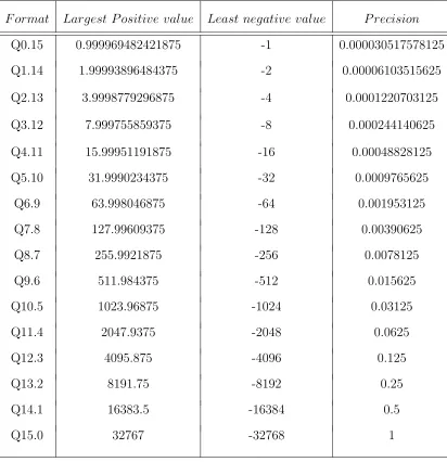
Fixed-point fractions are denoted using the Q-format where Q denotes Quantity of Fractional bits [27]. Qm.n indicates m bits for the integer while n denotes the number of bits devoted to the fractional part. A 16-bit fraction is denoted by Q0.15 (or Q.15) while the 16-bitintegerrepresentation is Q15.0. There is a trade-off between the dynamic range and precision of a fixed point representation. While Q0.15 has the highest precision (2−15) and the least dynamic range (+1), Q15.0 has the highest
the dynamic range and precision of all possible Qm.n formats possible with 16-bit
representation [28].
Table 4.1: Dynamic Range/Precision chart for 16-bit Q-formats
F ormat Largest P ositive value Least negative value P recision
Q0.15 0.999969482421875 -1 0.000030517578125
Q1.14 1.99993896484375 -2 0.00006103515625
Q2.13 3.9998779296875 -4 0.0001220703125
Q3.12 7.999755859375 -8 0.000244140625
Q4.11 15.99951191875 -16 0.00048828125
Q5.10 31.9990234375 -32 0.0009765625
Q6.9 63.998046875 -64 0.001953125
Q7.8 127.99609375 -128 0.00390625
Q8.7 255.9921875 -256 0.0078125
Q9.6 511.984375 -512 0.015625
Q10.5 1023.96875 -1024 0.03125
Q11.4 2047.9375 -2048 0.0625
Q12.3 4095.875 -4096 0.125
Q13.2 8191.75 -8192 0.25
Q14.1 16383.5 -16384 0.5
Q15.0 32767 -32768 1
The Q0.15 fixed point format is chosen for data representation in the BFPIALU
in order to obtain maximum precision. Figure 4.1 illustrates the Q0.15 two’s com-plement fixed point binary format and the weights associated with each bit position.
represent the fraction.
Figure 4.1: Two’s complement Q0.15 fixed point representation
4.2
Operations in the Q0.15 format
Operations using the Q0.15 data format are classified into
• Arithmetic operations
• Logical operations
• Comparison operations
• BFP operations
We discuss each category of operations in order starting with the basic arithmetic
operations of addition, subtraction and multiplication in the Q0.15 format. We then follow it up with a discussion of Logical, Comparison and BFP operations.
4.2.1
Arithmetic Operations
Arithmetic operations of addition and subtraction face the problem of overflow.
The operation of multiplication does not result in bit growth on the MSB side because
the product of two fractions is also a fraction. However, overflow errors are faced in the operation of multiply-accumulate. We illustrate these operations first for cases
that do not lead to overflow in order to retain focus on the operation performed. We
A. Arithmetic Operations without Overflow
i) Addition
Addition in Q0.15 involves direct binary addition for the arguments involved.
EXAMPLE 1
1. (0.15625) + (0.78515625) = 0.94140625
0 . 0 0 1 0 1 0 0 0 0 0 0 0 0 0 0 (+0.15625) +
0 . 1 1 0 0 1 0 0 1 0 0 0 0 0 0 0 (+0.78515625)
————————————————————–
0 . 1 1 1 1 0 0 0 1 0 0 0 0 0 0 0 (0.94140625)
EXAMPLE 2
2. (-0.15625) + (-0.78515625) = -0.94140625
1 . 1 1 0 1 1 0 0 0 0 0 0 0 0 0 0 (-0.15625) +
1 . 0 0 1 1 0 1 1 1 0 0 0 0 0 0 0 (-0.78515625)
————————————————————–
ignore
1 1 . 0 0 0 0 1 1 1 1 0 0 0 0 0 0 0 (-0.94140625)
The MSB in Example 2 is ignored because the bit in the MSB position bears the
same sign as the inputs.
ii) Subtraction
Subtraction is done by computing the two’s complement of the subtrahend and
EXAMPLE 1
1. (0.78515625) - (0.15625) = 0.62890625
0 . 1 1 0 0 1 0 0 1 0 0 0 0 0 0 0 (+0.78515625) +
1 . 1 1 0 1 1 0 0 0 0 0 0 0 0 0 0 (-0.15625)
—————————————————————–
ignore
1 0 . 1 0 1 0 0 0 0 1 0 0 0 0 0 0 0 (0.62890625)
EXAMPLE 2
2. (0.15625) - (0.78515625) = -0.62890625
0 . 0 0 1 0 1 0 0 0 0 0 0 0 0 0 0 (+0.15625) +
1 . 0 0 1 1 0 1 1 1 0 0 0 0 0 0 0 (-0.78515625) —————————————————————–
ignore
0 1 . 0 1 0 1 1 1 1 1 0 0 0 0 0 0 0 (-0.62890625)
We ignore the MSB in the result of both these examples because the input arguments
to the addition operation bear different signs and therefore, they do not overflow.
iii) Multiplication
The multiplication of two N-bit two’s complement numbers always results in a
2N-bit result. Multiplying two f1,15 or Q0.15 numbers produces a product in the f2,30
format and this can be reduced to f1,31 format by introducing a 0 in the LSB and
ig-noring the extra sign bit in the actual product. With interval multiplication, outward rounding is required on the interval product to ensure that all possible products for
point-wise evaluations with points drawn from the input intervals are contained [9]. Therefore, the excess bits of precision in the lower endpoint of the product are
dis-carded to fit the output word size. The upper endpoint is rounded to +∞ by adding
The following examples illustrate this operation.
EXAMPLE 1
0. 125 * 0.5625 = 0.0703125
0.001000000000000 * 0.100100000000000
= 00.000100100000000000000000000000 = 0.0001001000000000000000000000000
Upon rounding to 16-bits, the product would be 0.000100100000000.
EXAMPLE 2
0.9375 * 0.15625 = 0.146484375
0.111100000000000 * 0.001010000000000 = 00.001001011000000000000000000000
= 0.0010010110000000000000000000000
Upon rounding to 4-bits, the product would be 0.010.
The operation of multiplication is performed between positive values only. If any
argument is negative, it’s two’s complement value is taken and then the multiplication
is performed. The result is negated again if only one of the input arguments bore a
negative value. This step is not undertaken if both arguments are positive or if both arguments are negative. An XOR between the sign bits of the arguments indicates
whether the last step is performed or not.
B. Arithmetic Operations with Overflow
Overflow occurs when the true representation of the result requires more bits on the MSB side than the number of bits actually available. The following section
i) Overflow Detection Scheme in Addition
Overflow is detected for the addition operation involving two arguments x and y when both the following conditions are satisfied: [29]
• Bothx and y bear the same sign
• The sign of the output is not equal to the sign of the inputs
The following examples illustrate overflow for addition. Consider two positive
argu-ments 0.75 and 0.5 under the Q0.15 fixed point format. Adding these arguargu-ments
should lead to an overflow since the sum 1.25 exceeds the highest representable value of +(1-2−15).
EXAMPLE
0 . 1 0 0 0 0 0 0 0 0 0 0 0 0 0 0 (0.5) +
0 . 1 1 0 0 0 0 0 0 0 0 0 0 0 0 0 (0.75)
—————————————–
1 . 0 1 0 0 0 0 0 0 0 0 0 0 0 0 0 (-0.75)
The sign of the result has changed with respect to the inputs; the sign of the result is negative while bothxand yare positive. This is a clear indicator of overflow and the resulting value is -0.75 which is incorrect. In this case, the additional bit on
the MSB side must be captured by using a Guard bit and the whole result should
be right shifted by one position. The Guard bit is one additional bit provided to capture single bit growth beyond the MSB of the result. Figure4.2 shows the scheme to capture the bit growth, This would yield the final result to be 0.101000000000000 which corresponds to 0.625 at half the original scale. An XOR between the signs of
the input arguments indicates if they are of the same sign or not. An XOR between
the signs of the output and any one of the inputs indicates if the second condition
Consider the addition of two negative numbers (-0.5) and (-0.75).
EXAMPLE
1 . 1 0 0 0 0 0 0 0 0 0 0 0 0 0 0 (-0.5) +
1 . 0 1 0 0 0 0 0 0 0 0 0 0 0 0 0 (-0.75)
———————————————————
1 0 . 1 1 0 0 0 0 0 0 0 0 0 0 0 0 (+0.75)
Wrap around about the negative extreme (-1) occurs since the result is less
than (-1), the smallest number representable. The value of the result is found to be +0.75 which is wrong. Therefore, it is scaled down by a factor of 2 to yield
1.011000000000000 which is (-0.625).
Figure 4.2: Capturing bit growth
The multiply-accumulate instruction performs an addition to accumulate the
product terms. Therefore, similar logic for overflow detection is applied to this
in-struction as well. However, the register size in this case is 33 bits with one guard bit and 32-bit product width.
ii) Overflow Detection Scheme in Subtraction
Given two arguments x and y, overflow is detected in (x-y ) if
• Bothx and (-y) are of the same sign
• The sign of the result is different from that of xand (-y)
EXAMPLE
0 . 1 1 0 0 0 0 0 0 0 0 0 0 0 0 0 (+0.75) +
0 . 1 0 0 0 0 0 0 0 0 0 0 0 0 0 0 (+0.5)
—————————————————————–
1 . 0 1 0 0 0 0 0 0 0 0 0 0 0 0 0 (-0.75)
In the example above, overflow is detected since the sign of the result is different
from that of the inputs. Therefore, the output needs to be scaled. The actual output
scaled by a factor of 2 will be 0.101000000000000 or 0.625 in decimal representation. The value of (-y) is computed by subtracting it from 0. Overflow occurs when both
conditions are true, and each condition is verified by an XOR operation between the
sign bits if the relevant inputs.
4.2.2
Logical Operations
The logical command set includes the operations of OR, AND and XOR. These operations are widely used for applications such as Error Control Coding. This is
demonstrated in the examples below.
EXAMPLE 1
OR operation
1 0 1 0 1 0 1 1 0 1 0 0 1 1 1 1
0 1 1 0 0 1 1 1 0 0 0 1 1 0 0 0 —————————————
1 1 1 0 1 1 1 1 0 1 0 1 1 1 1 1
EXAMPLE 2
AND operation
1 0 1 0 1 0 1 1 0 1 0 0 1 1 1 1
0 1 1 0 0 1 1 1 0 0 0 1 1 0 0 0 —————————————
EXAMPLE 3
XOR operation
1 0 1 0 1 0 1 1 0 1 0 0 1 1 1 1
0 1 1 0 0 1 1 1 0 0 0 1 1 0 0 0
————————————— 1 1 0 0 1 1 0 0 0 1 0 1 0 1 1 1
4.2.3
Comparison Operations
Comparison operations are encountered frequently in applications such as fuzzy
adaptive filtering [2]. They involve a comparison of corresponding endpoints of the argument intervals. The method of comparing two Q0.15 numbers to identify the
minimum among them is discussed next. The other number is the maximum.
Between a positive number and a negative number, the minimum is identified as
the one with the sign bit ‘1’. Between two positive or two negative numbers, an
unsigned comparison of the numbers yields the minimum of the two.
EXAMPLE 1
min(1.010101101001111, 0.010001100001000) = 1.010101101001111
EXAMPLE 2