Morse homology
Shuaige Qiao
u5693534
May 2016
Declaration
Abstract
Morse homology were developed during the first half of the twentieth century. The underlying idea and various infinite dimensional versions, such as Floer homology, continue to be of interest to researchers in mathematics and theoretical physics today.
In the first chapter of this thesis, we briefly describe the finite dimensional Morse theory and its cellular singular homology . Our main focuses are sta-ble/unstable manifolds, the associated CW-complex. Suppose M is a smooth compact finite dimensional Riemannian manifold and f is a real valued function defined on M with all critical points nondegenerate. We consider the gradient flow line, that is, a smooth curve γ :R →M satisfying the following differential equation:
dγ(t)
dt +5f(γ(t)) = 0
Using these graident flow lines, we can decompose M into cells and construct a CW-complex associated tof.
In chapter two, we introduce Morse homology, whose chain complex is gen-erated by critical points of f and the boundary operators is defined by counting certain gradient flow lines connecting two critical points of relative index one. In order to check that this boundary is well-defined, We need to study the analysis of moduli spaces of gradient flow lines. These moduli spaces can be identified as zero sets of some Fredholm operators between infinite dimensional Banach man-ifolds. Since the moduli spaces may fail to be compact, we will discuss about the compactification of the moduli space. Then we obtain the fact that there are finitely many flow lines between critical points with relative index 1. After defining an coherent orientation on moduli spaces, we can construct boundary op-erator of Morse complex by counting flow lines with sign. This approach is very useful in studying a generalization of Morse theory on certain infinite-dimensional manifolds.
In chapter 3, we show that the two kinds of homology we construct in the
previous two chapters are isomorphic. In fact, we show that two chain complexes are identical.
Contents
Abstract v
Notation ix
1 Cellular Homology 1
1.1 Brief review of Morse theory . . . 1
1.2 The CW complex associated to a Morse-Smale function . . . 3
1.2.1 The unstable manifold theorem . . . 3
1.2.2 Morse-Smale condition . . . 5
1.2.3 The attaching map . . . 6
1.3 Cellular homology of M . . . 10
2 Morse Homology 13 2.1 The space of gradient flow lineµx,y . . . 13
2.2 Fredholm property . . . 16
2.3 Transversality theorem . . . 21
2.4 Moduli space ofµx,y . . . 24
2.5 Compatification of ˆµx,y . . . 26
2.6 Gluing . . . 29
2.6.1 Pre-gluing . . . 30
2.6.2 The construction of gluing map] . . . 33
2.6.3 Conclusion . . . 38
2.7 Orientation . . . 38
2.7.1 The determinant line bundle . . . 38
2.7.2 Orientation on glued Fredholm operators . . . 42
2.7.3 Coherent orientation on µx,y . . . 45
2.7.4 Orientation on W(x, y) . . . 46
2.8 Morse complex . . . 47
3 Morse complex agrees with cellular complex 49
4 An overview of Floer theory 53
4.1 Lagrangian-Floer theory . . . 53 4.2 Instanton Floer theory . . . 56
Notation
H1,2(
R,Rn) Sobolev space of curves square-integrable together with the first derivative
Cx,y∞ smooth curves with ends x, y
L(X,Y) space of continuous linear Banach space operators K(X,Y) space of compact operators
F(X,Y) space of Fredholm operators between Banach spaces Cloc∞ space of smooth function withC∞-compact-open topology
Chapter 1
Cellular Homology
1.1
Brief review of Morse theory
The main goal of Morse theory is to show how to construct a CW-complex that is homotopy equivalent to a smooth manifold M using “Morse function”. More precisely, we can uncover the information about the topology of M by discussing the critical point of Morse function. Morse theory plays an important role in classifying smooth manifolds. Floer in 1980s developed an infinite dimensional version of Morse theory and our understanding of low dimensional manifolds and symplectic topology. This will be introduced briefly in chapter 4.
We first introduce some definitions.
Definition 1.1. Let M be a smooth compact finite dimensional manifold and f :M →R
is a smooth map. Then a point p is called acritical point if the following differ-ential map
dfp :TpM →Tf(p)R∼=R
is zero.
If p is a critical point of f, we can define a symmetric bilinear form Hesspf
onTpM,which is called the Hessian of f atp.
Hesspf :TpM ×TpM →R
In terms of local coordinate chart {x1, x2, ..., xn} near p, Hesspf is the familiar
matrix of second partial derivatives Hesspf = (
∂2f ∂xi∂xj
(p))
A critical point p is called non-degenerate if Hesspf is nonsingular. It is easy
to check that the non-degeneracy does not depend on the coordinate system. A function with all its critical point nondegenerate is called Morse function. We can now talk about the index of f atp.
Definition 1.2. Theindex of a critical point p, denoted as λ(p), is the maximal dimension of a subspace of TpM on which Hesspf is negative definite.
From linear algebra, it is obvious that the index of a critical point p is ex-actly the number of the negative eigenvalue of the Hessian matrix at p. Now we introduce the Morse lemma, which shows that the behaviour of f near pcan completely described by the index.
Lemma 1.3. (Morse lemma) Suppose p is a non-degenerate critical point of f, then ∃ local coordinate chart (x1, x2, ..., xn) near p s.t. xi(p) =o for all i and
f =f(p)−x21−...−x2λ+x2λ+1+...+x2n where λ=λ(p), n =dimM.
Then we have the following theorem describing the CW-complex associated to a Morse function.
Theorem 1.4. If f ∈C∞(M,R) is a Morse function and M is compact smooth and finite dimensional. Then M has the homotopy type of a CW-complex, with one cell of dimension λfor each critical point of indexλ,i.e.,M 'S
x∈critkfe
λ(x)
x .
We denote the set of all points whose function value is less or equal to a by Ma, i.e., Ma ={x :f(x)≤ a}.The key observation which finally proved this
theorem is the change of the homotopy type ofMawhenacrosses a critical value.
The proof of this theorem and Morse lemma is given in Milnor’s “Morse theory”. As a concequence, if we denote the Betti number and numbers of critical points of index k by:
bk =dimHk(M,R) k = 0,1, ..., n=dimM
ck =]critkf crittf ={x∈critf :λ(x) =k}
Then the following “Morse inequalities” hold:
ck−ck−1+...±c0 ≥bk−bk−1 +...±b0 k= 0, ..., n−1
1.2. THE CW COMPLEX ASSOCIATED TO A MORSE-SMALE FUNCTION3
1.2
The CW complex associated to a
Morse-Smale function
Morse theory has described how a compact finite dimensional manifold M is homotopy equivalent to a CW complex. It would be nice if we could describe the manifold as a CW complex directly, instead of homotopy equivalence. We will see that only Morse function is not enough to accomplish this, and we also need a transversality condition which is called Morse-Smale condition. To do this, we first show how the cells of the CW complex come from.
1.2.1
The unstable manifold theorem
SupposeM is a finite dimensional compact Riemannian manifold andf is a Morse function defined on M and x ∈ M. Let γx(t) be a flow line through x, i.e., it
satisfies the following differential equation: ∂
∂t(γ) =− 5f(γ) γx(0) =x
Then for any critical point p, we can have the stable and unstable manifolds defined by:
Ws(p) ={x∈M : lim
t→+∞γx(t) =p} Wu(p) ={x∈M : lim
t→−∞γx(t) =p}
In other words, the stable manifold is the set of points in M that flow down to p, and the unstable manifold is the set of points that flow up to p. We now state a theorem that explains the term “manifold” in these two definitions. Theorem 1.5. Let f be a Morse function and (M, g) be a compact smooth and n-dimensional Riemannian manifold. Then for any critical point p ∈ M of f with λ(p) = λ, we have
TpM =TpsM
M
TpuM
where the Hessian is positive definite on Ts
pM and negative definite on TpuM.
Moreover, Ws(p) and Wu(p) are smoothly embedded open disks of dimension
equal to n−λ and λ respectively.
The proof of theorem 1.5 is given in chapter4 of [1].
Proposition 1.6. If(M, g)is a compact Riemannian manifold, andf is a Morse function on M, then
M = G
p∈crit(f)
Wu(p)
Proof. For any x∈M, consider the flow lineγx(The existence and uniqueness of
γx come from the result of Lemma 2.4 in Milnor’s “Morse theory”). Then f◦γx
is a function from R toR.
By the fundamental theorem of caculus, (f◦γx)(b)−(f◦γx)(a) =
Z b
a
d
dt(f◦γx)(t)dt
f ◦γx is bounded since M is compact, so the left-hand side of the fomula is
bounded. For right-hand side, we have
d
dt(f◦γx) = <5(f ◦γx), γ 0
x >
= <5(f ◦γx),− 5(f ◦γx)>
= − | 5(f◦γx)|2
≤ 0 (1.1)
Therefore,
lim
t→±∞ d
dt(f ◦γx)(t) = 0 So,
lim
t→±∞− | 5f(γx(t))|
2
= 0 SinceM is compact,M−S
p∈crit(f)Up is compact, where Up is a small
neigh-bourhood of p. So | 5f |2 has its minimum on M − S
p∈crit(f)Up, which is
positive since there is no critical point onM−S
p∈crit(f)Up. We have proved that
the limit of | 5f(γx(t))|2 is zero, so when the absolute value of t is sufficiently
large, γx(t)∈
S
p∈crit(f)Up.
The limits of γx(t) are critical points since we can make Up arbitrary small.
As a concequence,
M = [
p∈crit(f)
Wu(p)
Wu(p)T
Wu(q) =∅ when p6=q comes from the uniqueness of γ x.
1.2. THE CW COMPLEX ASSOCIATED TO A MORSE-SMALE FUNCTION5
1.2.2
Morse-Smale condition
Definition 1.7. Suppose (M, g) is a finite dimensional smooth Riemannian man-ifold, and f :M →R is a Morse function. f is called a Morse-Smale function if for all p, q ∈crit(f)
Ws(p)tWu(q).
Given Morse-Smale condition, we can see how unstable and stable manifolds of different critical points intersect. For any two critical pointsp, q, we will denote
Wu(p)\Ws(q) = W(p, q)
W(p, q) is the space of points that flow from p toq. Then we have the following proposition.
Proposition 1.8. Suppose (M, g) is an n-dimensional compact smooth mani-fold, and f is a Morse-Smale function defined on M. Then ∀p, q ∈ crit(f), if W(p, q)6=∅, W(p, q) is a submanifold of M of dimension λ(p)−λ(q).
Lemma 1.9. The intersection of two transversal submanifolds of Y, say X and Z, is again a submanifold. Moreover,
codim(X∩Z) =codim(X) +codim(Z)
The proof of lemma 1.9 can be found in section 1.5 of [3].
Proof. (of propositon 1.8) From theorem 1.5 we know Wu(p) and Ws(q) are
smooth embedded submanifold of dimension λ(p) and n−λ(q). Since Ws(p) t
Wu(q), by lemma 1.9, we know W(p, q) is a submanifold and
codim(W(p, q)) =codim(Wu(p)) +codim(Ws(q))
⇒dim(W(p, q)) =λ(p)−λ(q)
IfW(p, q)6=∅, then it contains at least one flowline fromptoq, which means that W(p, q) can not be zero-dimensional. Thus, we can immediatly have the following corollary.
Corollary 1.10. SupposeM, f, p, qare defined the same as above, thenW(p, q)6=
We refer to the number λ(p)−λ(q) as the relative index of p and q.
In 1963, Kupka and Smale proved that Morse-Smale gradient vector fieds are generic. We now state the theorem but the proof of this theorem will be shown later in chapter 2 after we construct the flow line space by Fredholm system. Once we have this propoty of Morse-Smale condition, we can change a Morse function to a Morse-Smale function by perturb the metric a little bit.
Theorem 1.11. SupposeM is a smooth compact finite-dimensional manifold and f is a Morse function defined on M, then for a generic Ck-smooth metric g on
M, the submanifold Wu(p) and Ws(q) intersect transversally, i.e.,
Wu(p)tWs(q) ∀p, q ∈crit(f)
1.2.3
The attaching map
We have seen that Wu(a) is λ(a)-cell of M for each critical point a, while to
define the attaching map, it is convinient to treat a little neighbourhood of a in Wu(a) as the λ(a)-cell rather than the whole unstable submanifold. To see this,
we derive the following theorem.
Theorem 1.12. Suppose (M, g) is a Riemannian manifold and f :M →R is a Morse function. Let a be a critical point of f with index λ and f˜: Wu(a) → R
be the restriction of f on Wu(a). Then
i) a is the unique critical point of f˜and f˜(a) is the absolute maximum. ii) f˜−1 ( ˜f(a)−,f˜(a)) is diffemorphic to a λ-disk for some small . iii) ∂f˜−1 ( ˜f(a)−,f˜(a))
= ˜f−1( ˜f(a)−)∼=Sλ−1
Proof. ∀x∈Wu(a)\{a}, we have lim
t→−∞=a Then from (1.1) we know that
d
dt(f ◦γx) =− | 5(f◦γx)|
2<0
Sincex6=a, the image ofγxdoes not contain critical points off, so the derivative
can not be zero. Thus f(γx(t)) is strictly decreasing. By the continuity of f, we
have
lim
1.2. THE CW COMPLEX ASSOCIATED TO A MORSE-SMALE FUNCTION7
Therefore,f(a)> f(x), i.e., a is the absolute maximum of ˜f.
For all t ∈ R, γx(t) ∈ Wu(a), so γx0(0) ∈ TxWu(a). Since f(γx(t)) is strictly
decreasing, γx0(0) 6= 0, so 5xf 6= 0. Therefore x /∈ crit( ˜f), i.e., a is the only
critical point of ˜f.
Now, we want to show ˜f is a Morse function. Choose a coordinate chart of M near a such that xλ+1 = ... = xn = 0 on Wu(a). Since Hess(f) is negative
definite on TxWu(a), the matrix
∂2f
∂xi∂xj
ij
is negative definite on TxWu(a). Since xλ+1 =...=xn = 0,then for i, j ≤λ, the
Hessian matrix of f is the same as
∂2f˜
∂xi∂xj
ij
SoHess( ˜f) is negative definite. We can now conclude that ˜f is a Morse function. Apply Morse lemma on ˜f, there exists a neighbourhood U ⊆ Wu(a) near a and a coordinate chart (x1, ..., xλ) such that
˜
f(b) = ˜f(a)−x21(b)−...−x2λ(b) x1(a) =...=xλ(a) = 0
Let > 0 be small enouph so that Dλ() = {(x
1, ...xλ) | x21 +...+x2λ <
} ⊆ U. It is clear that Dλ() ⊆ f˜−1 ( ˜f(a)−,f˜(a))
. Now we want to show ˜
f−1 ( ˜f(a)−,f˜(a))
⊆Dλ().
If x ∈ Wu(a), and x /∈ Dλ(), since a ∈ Dλ() and lim
t→−∞γx(t) = a,
γx(t) ∈ Dλ() for some t < 0. Then γx(T) ∈ ∂Dλ() for some T < 0(By the
Jordan-Brouwer separation theorem). Since f(x) =f γx(o)
< f γx(T)
=f(a)− then
x /∈f˜−1 ( ˜f(a)−,f(a))˜ So ˜f−1 ( ˜f(a)−,f(a))˜
⊆Dλ(). This shows ii) and iii).
For each critical point, the corresponding stable manifold has similar propoties. Then we denoteWs(a)T
f−1 (f(a), f(a)+)
asdna−λ(a)andWu(a)Tf−1 (f(a)−
, f(a)) aseλa(a), which is the λ(a)-cell of the CW-complex we are constructing.
Theorem 1.13. Let (M, g) be a smooth compact n-dimensional Riemannian manifold and f : M → R be a Morse-Smale function. p, q ∈ crit(f) and λ(p) = k+ 1, λ(q) =k, W(p, q)6=∅, i.e., ∃γ :R→M such that
lim
t→−∞γ(t) =p t→lim+∞γ(t) = q Denote γ(R)T
∂ek+1
p as α. Then there exists a neighbourhood Opγ of α in ∂ekp+1,
i.e., α∈Oγ
p ⊆∂ekp+1 and a homeomorphism
ϕγp,q:Oγp →ekq
To prove this theorem, we first introduce a lemma.
Lemma 1.14. Let (M, g), p, q be defined the same as those in theorem 1.13, then there exists a neighbourhood U of q and a coordinate chart x = (x1, ..., xn) such
that x(U) =Dk()×Dn−k() and
x|ek
q :e
k q →D
k× {0}
x|dn−k
q :d
k
q → {0} ×D n−k
are diffeomorphisms.
Proof. By Morse lemma, we know that there exists a neighbourhood V of q and a coordinate chart (x1, ..., xn) on V such that
f(p) =f(q)−x21−...−x2k+x2k+1+...+x2n x1(q) =...=xn(q) = 0
Let >0 be small enough such that
Dk()×Dn−k()⊆V Let U =x−1 Dk()×Dn−k()
, then
x−1 Dk(× {0}) = {p∈U |x(p) = (x1, ..., xk,0, ...,0) x12+...+x2k < }
= Wu(q)\f−1 (f(q)−, f(q))
= ekq Similarly,
1.2. THE CW COMPLEX ASSOCIATED TO A MORSE-SMALE FUNCTION9
Proof. (of theorem 1.13) We construct ϕγ
p,q by two steps: first, we define a map
from the plague Oγ
α 3 α diffeomorphically to a plague O γ
β 3 β (readers can see
what β is intuitively in the figure 1.1, we will define β rigorously in the following proof); Second, we define a map from Oβγ toek
q.
Figure 1.1 Since γ is a flow line fromptoq, thenγ(R)T
dn−k
q 6=∅. Letβ ∈γ(R)
T
dn−k q .
Step 1: Choose a little plague Oγ
α of α in ∂ekp+1. Since ∂ekp+1 ∼= Sk, then
Oγ
p ∼=Dk. Since α, β ∈γ(R), β =γα(T) for some T > 0. Then we define ϕ1 on
Oγ α by
ϕ1(r) =γr(T)
Then ϕ1 is a diffeomorphism(Since γx(t) is generated by a smooth vector field 5f). Thus Oγβ =ϕ2(Oγα) is diffeomorphic toDK.
Step 2: Choose a neighbourhood Tγ([T,∞]) of γ([T,∞]) such that
i) Tγ([T ,∞]) ⊆U, where U is defined in lemma 1.14.
ii) There exists an diffeomorphism ψ : Tγ([T ,∞]) → [0,1]×Dn−k−1()×Dk()
such that for all t≥T
ψ γ(t) = t−T t ,0,0
∈[0,1]×Dn−k−1()×Dk() ψ Oβγ = {0} × {0} ×Dk
[image:19.595.175.483.190.447.2]Then we define ϕ2 :Oγβ →ekq by the following diagram
This diagram commutes, and it is obvious thatϕ2 is a diffeomorphism.
Suppose critk(f) ={q1, ..., qs}, then we define the attaching map
ϕ:∂ekp+1→ s
[
i=1
ekqi
by
ϕ(r) =
ϕγ
p,qi(r) r∈O
γ
α for some γ that flows from p toqi
∗ otherwise
1.3
Cellular homology of M
Denote the k-skeleton byXk, then
Xk = G
p∈criti(f),i≤k
eip.∼
where the equivalence relationship comes from the attaching map. Then we define the boundary map by
i) Whenk = 1, the boundary map∂C
1 :H1(X1, X0)→H0(X0) is the same as
the simplicial boundary map. ii) Whenk > 1,
∂kC(ekp) = X
q∈critk−1(f)
1.3. CELLULAR HOMOLOGY OF M 11
where αpq is the map
∂ekp →Xk−1 →Sqk−1
that is, the composition of the attaching map of ek
p with the quotient map
collapsing Xk−1\ek−1
q to a point.
Now we have the cellular chain complex: Ck =
M
p∈critk(f)
Chapter 2
Morse Homology
2.1
The space of gradient flow line
µ
x,yIn the previous chapter, we have introduced the dynamical system given by the negative gradient flow of a Morse-Smale function. Now we continue to study more about the gradient flow line space, which is needed for the definition of Morse homology.
Definition 2.1. Let M be an n-dimensional compact manifold, f : M → R a Morse-Smale function. Then we define the gradient flow line space as follow
µx,y ={γ ∈C∞(R, M)| lim
t→−∞γ(t) = x,t→lim+∞γ(t) =y, γ 0
(t) =− 5f(γ)}
µx,y can be seen as the space of zeros of a section of a fredholm system. To
see this, we first define the Banach space and Banach bundle.
Definition 2.2. LetE be a smooth, finite-dimensional vector bundle over ¯R(the compatification of R) and let φ :E →R¯ ×Rn be a smooth trivialization. Then
φ∗ is the induced one-to-one map between the associated vector space, i.e. φ∗ : Γ( ¯R, E)→C0( ¯R,Rn)
Then we define
H1,2(E) = φ−∗1(H1,2(R,Rn)) Since the Sobolev space H1,2(
R,Rn) is a Banach space, φ∗ induces a Banach space topology on the vector space H1,2(E). The following proposition shows
that this topology is independent of the choice of the trivialization φ, for the change of trivialization from φ to ˜φ can be represented by some A = ˜φ◦ φ ∈
C1( ¯
R, GL(n,R)).
Proposition 2.3. ∀A∈C1( ¯
R, GL(n,R)),∃c >0 s.t.
kAsk1,2≤cks k1,2 ∀s∈H1,2(R,Rn)
where (As)(t) = A(t)·s(t), t∈R.
Proof. It is sufficient to show Aij and A0ij are bounded.
∀f ∈C1( ¯R,R),f is obviously bounded. Defineh: ¯R→[−1,1] byh(t) = √t
1+t
then f ◦h−1 ∈C1([−1,1],R). Then c(f) = sup
[−1,1]
|(f◦h−1)0 |<∞
Since
((h−1)0◦h)(t) = (1 +t2)32
(f ◦h−1)0 =f0◦h−1·(h−1)0 thenc(f)≥|f0(t)|(1+t2)32, i.e. |f0(t)|≤ c(f)
(1+t2)32, which impliesf
0 is bouned. We now give a brief definition of the Banach manifold in the Fredholm sys-tem we have previously mentioned. We start with the exponential map on the complete Riemannian manifold M.
Let D be an open convex neighbourhood in the zero section of T M. Then
∀h ∈ C∞( ¯R, M), h∗D stands for the induce open convex neighbourhood of the zero section in the pull-back bundleh∗T M. By the Sobolev embedding, we define
Px,y1,2 ={exp◦s ∈C0( ¯R, M)|s∈H1,2(h∗D), h∈Cx,y∞( ¯R, M)}
where exp◦s(t) = exph(t)s(t). Then Px,y1,2 is equipped with a Banach manifold
structure via the atlas {H1,2(h∗D), exph}h∈C∞
x,y( ¯R,M). For more details of the fact,
see Appendix A of [7]. Similarly, we can define
L2(E) = φ−∗1(L2(R,Rn))
which is also a Banach space since L2(R,Rn) is a Banach space. This leads to the Banach bundle over Px,y1,2
L2(Px,y1,2∗T M) = [
s∈Px,y1,2
L2(s∗T M)
2.1. THE SPACE OF GRADIENT FLOW LINE µX,Y 15
Theorem 2.4. Given a section
F :Px,y1,2 → L2(Px,y1,2∗T M) s 7→ s˙+5f◦s Then F−1(0) =µx,y
Proof. We proveµx,y ⊆F−1(0) first. By assumption, elements ofF−1(0) are
con-tinuous curves withx, y as its end points whose weak derivative can be expressed as
˙
s=− 5f ◦s It follows that µx,y ⊆F−1(0).
To see F−1(0) ⊆µ
x,y, we introdce the following lemma:
Lemma 2.5. (Exponential decay to critical points)There exists an > 0 such that ∀s∈F−1(0),∃c >0 and t
0 >0 satisfying
d(s(t), y)≤ce−t ∀t ≥t0 d(s(t), x)≤ce−t ∀t ≤ −t0
Proof. (of lemma) By Morse lemma, we can find a neighbourhood U of y and equip a Morse chart on it. Without loss of generality, assume f(y) = 0, then
f(z) =
k
X
i=1
zi2− n
X
i=k+1
zi2 ∀z ∈U
and accordingly:
5f(z) = (2z1, ...,2zk,−2zk+1, ...,−2zn)
k 5f(z)k2= 4
n
X
i=1
zi2 ≥4|f(z)−f(y)|
Since lim
t→+∞s(t) =y, zi(o) = 0 for i = k+ 1, ..., n, it is clear that for such an s, it must exponentially decay to 0 as t → +∞ since ∂s(t)
∂t =− 5f(s(t)), i.e. for t >0
∂zi(t)
∂t =−2zi(t) i= 1, ..., k ∂zi(t)
∂t = 2zi(t) i=k+ 1, ..., n The proof of the result of x is similar.
Now, we have managed to represent the flow line space as a zero set of a smooth section of a Banach bundle over a Banach manifold. To proceed to the manifold property of µ(x, y), we need to develop the Fredholm property of a certain linear first order differential operator Fγ, which is defined in the following
section.
2.2
Fredholm property
Suppose s is a vector field along γ ∈Cx,y∞( ¯R, M), and s(t)∈Tγ(t)M, we define
Fγ :H1,2(R, γ∗T M) → L2(R, γ∗T M) s 7→ 5ts+5s5f(γ)
where 5 is the covariant derivative.
Theorem 2.6. Fγ is a Fredholm operator and
ind(Fγ) = ind(x)−ind(y)
The proof of this theorem requires the following observation:
Lemma 2.7. Let X, Y, Z be Banach spaces, suppose F ∈ L(X, Y) and K ∈
L(Y, Z). If ∃c >0, s.t.∀x∈X
kxkX≤c(kF xkY +kKz kZ)
then dimkerF <∞ and the image of F is closed.
Proof. The proof consists of two parts: i) We first show thatdimkerF <∞.
By Riesz’s lemma, it suffices to show that the unit ball in the kernel of F is compact.
Let{xn}∞n=1 be a sequence in the unit ball of kerF, i.e.
kxkX≤1 F(xn) = 0 ∀n ∈N
then the hypothesis becomes:
kxkX≤ckKz kZ
2.2. FREDHOLM PROPERTY 17
complete). Then {xn} is Cauchy and hence converges in X and therefore in the
unit ball. This proves the compactness of the unit ball in kerF. ii) We now show that Im(F) is closed in Y.
Let{xn}∞n=1 be a sequence inX s.t. limn→∞F(xn) =y ∈Y, we want to show
that y∈Y.
If {xn}∞n=1 is bounded, then {Kxn}∞n=1 remains in a compact subset of Y.
Along with L(xn)→y and the inequality
kxkX≤c(kF xkY +kKz kZ)
it follows that{xn}∞n=1 has a Cauchy subsequence, hence converges and the limit
x satisfies y=F(x). So y∈Im(F).
If {xn}∞n=1 is unbounded. Since kerF is finite-dimensional, we can find a
closed subspace E ⊆ X s.t. kerF ⊕E = X. Consider the sequence un = kxxnnk,
without loss of generality, we can assume
{un} ⊆E kF un kY→0 as n→ ∞
Since {un} is bounded, there exists u such that
un→u kuk= 1 F u= 0
Sou∈kerF ∩E ={0}, which contradicts kuk= 1.
Equipped with the lemma, we can now prove theorem 2.6. Proof. i) We first prove that dimkerFγ<∞.
Let X = H1,2(
R, γ∗T M), Y = Z = L2(R, γ∗T M), F = Fγ, K : s 7→ s·δT,
where
δT =
1 t ∈[−T, T] 0 t /∈[−T, T]
Then X, Y, Z, F, K satisfy lemma 2.7. So it is sufficient to show that ∃c, T > 0 s.t.
Z
R
(|s|2 +| 5s|2)dt≤c(
Z
R
|Fγs |2 dt+
Z T
−T
|s |2 dt) (2.1) We first trivialize the bundles X, Y, Z. Let e1(t), e2(t), ..., en(t) be an orthonomal
basis of Tγ(t)M for all t ∈ R which satisfies that 5ei(t)≡ 0 for i = 1, ..., n. Let
(s1, ..., sn)∈Rn be the coordinates of s with respect to this basis. Then
Fγ(s) = Fγ
X
i
siei
= X
i
(dsi dt +
X
j
Let aij(t) =hei,5ej 5f(γ)i and A= (aij)n×n, thenA is a symmetric matrix.
We denoteFγ by
Fγtriv :H1,2(R,Rn) → L2(R,Rn) s = (s1, ..., sn) 7→
ds
dt +A·s,ϕ
Note thatA± = limt→±∞A(t) represents the Hessian off aty andxrespectively. Then A+ and A− are nonsingular forf is a Morse function. Consider the maps
Fγ,triv± :s7→ ds
dt +A±s,ϕ± By Fourier transformation,
ˆ
s(iω) = √1
2π
Z
R
eiωts(t)dt
then
ˆ
ϕ±(iω) = 1
√
2π
Z
R
eiωts(t)dt= √1
2π
Z
R
eiωt(ds
dt +A±s)dt = (iωI +A±)ˆs(iω)
Since A± are nonsingular, ∃c∈R s.t.
(1+|ω |2)|ˆs(iω)|2≤c|ϕ±(iω)ˆ |2
So ks k2
H1,2≤ckϕ± k2L2. This property holds for sufficiently small perturbation
of Ftriv γ,±.
For sufficiently large T, if s satisfies that s(t) = 0 for all t∈[−T, T], we then have the following estimate
ksk2
H1,2≤ckϕk2L2
On [−T −1, T + 1],
Z T+1
−T−1
|ϕ|2 =
Z T+1
−T−1
(| ds
dt |
2 +2hds
dt, Asi+|As |
2)dt
≥
Z T+1
−T−1
(1 2 |
ds dt |
2 − |As |2)dt
Since detA(t) is bounded on [−T−1, T+ 1], we obtain the following estimate for large enough cthat:
Z T+1
−T−1
(|s|2 +| ds
dt |
2
)dt≤c
Z T+1
−T−1
2.2. FREDHOLM PROPERTY 19
Now, let β be a cut-off function:
β(t) =
1 |t |≤T 0 |t |≥T + 1
and choose clarge enough so that |β0 |< c, then
ks kH1,2 ≤ kβskH1,2 +k(1−β)skH1,2
≤ c(kβskL2 +kFγtriv(βs)kL2 +kFγtriv((1−β)s)kL2)
Since
Fγtriv(βs) = d(βs)
dt +A·βs = dβ
dts+βF
triv γ (s)
we have:
kskH1,2 ≤ c(kβskL2 +2k
dβ
dtskL2 +kβF
triv
γ (s)kL2 +k(1−β)Fγtriv(s)kL2)
≤ 3c2(kβskL2 +kFγtriv(s)kL2)
This proves (2.1).
ii) It remains to show that Fγ has finite condimension and indFγ =ind(x)−
ind(y).
To see this, we compute the dimension of kerF directly and dimcokerFγ via
the adjoint operator ofFγ, relying on the result from part one thatFγ has closed
range. Consider
Fγtriv :s7→ 5s+As
(Fγtriv)∗ :s 7→ 5s−As
Since F(X, Y) is an open subset of L(X, Y) and the index is a locally constant function on F(X, Y), we can perturbe Fγtriv a little without changing its index.
Define
where P =
A(t)−A+ t∈[T,+∞)
(t−T)(A(t)−A+) t∈[T −1, T]
0 t∈[−T + 1, T −1]
(−T −t)(A(t)−A−) t∈[−T,−T + 1] A(t)−A− t∈(−∞,−T]
The norm of P can be arbitrarily small by makingT large enough. Thus, we can find a T >0 s.t.
indFγtriv =ind(Fγtriv+P)
Since A−, A+ are the Hessian of f at x, y respectively, then there exists
C+, C− ∈GL(n,R) and a curve C∈C∞( ˆR, GL(n,R)) s.t.
det(C±)>0
C±A±C±−1 =diag(λ±1, ..., λn±) where sgnλ±i ≥λ±i+1
f or some T >0, C(t) =C+ when t≥T and C− when t≤ −T Define C :s 7→C·s, then
C(Fγtriv+P)C−1 = C(5t+A+P)C−1
= 5t+C(5tC−1) +C(A+P)C−1
Since C, C−1 are invertible, the mapsC, C−1 are isomorphisms and we have indC(Fγtriv+P)C−1 =indFγ
For any initial value s0, the ODE
(C(Ftriv
γ +P)C
−1)s = 0
s(0) =s0
has unique solution on [−T, T].
On (−∞,−T) and (T,+∞), the equation becomes
5ts=−diag(λ−1, ..., λ
−
n)s 5ts=−diag(λ+1, ..., λ+n)
respectively. Thus, s satisfies
si(t) =
cie−λ −
it t <−T
die−λ
+
2.3. TRANSVERSALITY THEOREM 21
fori= 1, ...n. Sos∈kerC(Ftriv
γ +P)C
−1if and only ifλ−
i <0 andλ
+
i >0. Since
we have ordered the sign of eigenvalues and the number of negative eigenvalue of A± are the index of y, xrespectively, we can compute
dimkerFγ = ]{i∈ {1, ..., n} |λ−i <0, λ
+
i >0}
= max{ind(x)−ind(y),0}
Similarly,
dimcokerFγ = ]{i∈ {1, ..., n} |λ−i >0, λ
+
i <0}
= max{ind(y)−ind(x),0}
Therefore,indFγ =ind(x)−ind(y).
2.3
Transversality theorem
In this section we show that µx,y is a finite-dimensional manifold using the
Fred-holm property we discussed in last section. However this property is true only for a generic set of metrics. Also, Morse function turns out to be Morse-Smale function for a generic set of metric.
Theorem 2.8. Suppose G is the metric set on M, then there exists a generic subset Σ⊆G s.t. for all g ∈Σ, the section
Fg :Px,y1,2 → L
2(P1,2
x,y
∗ T M) s 7→ s˙+5f ◦s
is transversal to its zero section andFg−1(0) is a closed submanifold of dimension ind(x)−ind(y).
Theorem 1.11 follows from theorem 2.8. Proof. We extend Fg to a section
Φ :G×Px,y1,2 → L2(Px,y1,2∗T M) (g, s) 7→ (g, s, Fg(s))
Then from the previous discussion, Fg = Φ(g,·) is a Fredholm map with index
ind(x)−ind(y) for all g ∈G.
i) We first prove the manifold property of F−1
g (0)( i.e. µx,y).
Lemma 2.9. 0 is a regular value of Φ.
Proof. We want that ∀(g, s)∈Φ−1(0), the vertical differential
DΦ(g, s) :T(g,s)(G×B) → Es
(η, ξ) 7→ D1Φ(g, s)·η+D2Φ(g, s)·ξ
is surjective, where B =Px,y1,2, Es=L2(s∗T M).
Since D2Φ(g, s) = DFg(s) is a Fredholm operator, the image of DΦ(g, s) is
closed in L2 with finite codimension.
Suppose h∈L2(s∗T M) is orthogonal to the image of DΦ(g, s), i.e.
Z
R
hDΦ(g, s)(η, ξ), hidt= 0 ∀(η, ξ)∈T(g,s)(G×B)
Then it is sufficient to show that h= 0. Letη= 0, we get
Z
R
hDFg·ξ, hidt = 0 ∀ξ∈TsB
Then h can be expressed as the solution of some linear differential equation ˙
h(t) =X(t)h(t)
If h 6= 0, due to the uniqueness of solution of the ODE, h(t) 6= 0 for all t. So, letting ξ= 0, we have
Z
R
hD1Φ(g, s)·η, hidt= 0 h∈C∞, ∀η∈TgG (2.2)
Fix t0 ∈R, choose ξ s.t. D1Φ(g, s)·η = h(t0), then hD1Φ(g, s)·η, hi >0 at t0.
By the smoothness ofh, (2.2) can not be zero, which leads to a contradiction. Lemma 2.10. Let π : Φ−1(0) →G be the projection map, then π is a Fredholm
map of index ind(x)−ind(y).
Proof. All we need to show is that ∀(g, s)∈Φ−1(0), the following map
Dπ(g, s) :T(g,s)Φ−1(0) → TgG
(η, ξ) 7→ η
2.3. TRANSVERSALITY THEOREM 23
The isomorphism of kernels is shown by
ker(Dπ(g, s)) = {(0, ξ)∈TgG×TsB |(0, ξ)∈T(g,s)Φ−1(0), i.e.D2Φ(g, s)·ξ = 0}
∼= {ξ ∈T
sB |D2Φ(g, s)·ξ = 0}
= kerD2Φ(g, s)
For the cokernel part, consider the homomorphism induced by D1Φ(g, s)
g
D1Φ :coker(Dπ(g, s)) =TgG
.
Im(Dπ(g, s)) → coker(D2Φ(g, s)) = Es
.
Im(D2Φ(g, s))
[η] 7→ [D1Φ(g, s)·η]
Claim 1: Dg1Φ is a surjective.
For all v ∈ Es, by the surjectivity of DΦ(g, s) from lemma 2.9, there is
(η, ξ)∈T(g,s)G×B, such that D1Φ(g, s)·η+D2Φ(g, s)·ξ=v. Then
g
D1Φ([η]) = [D1Φ(g, s)·η] = [D1Φ(g, s)·η+D2Φ(g, s)·ξ] = [v]
Claim 2: Dg1Φ is an injective.
Suppose v ∈ Im(D2Φ(g, s)), then v = D2Φ(g, s)·ξ for some ξ ∈ TsB. If
η ∈ TgG satisfies D1Φ(g, s)·η = v, we have D1Φ(g, s)·η = D2Φ(g, s)·ξ, i.e.
(η,−ξ)∈T(g,s)Φ−1(0).
So η=Dπ(g, s)(η,−ξ)∈Im(Dπ(g, s)). Therefore Dg1Φ is an isomorphism.
Now we continue the proof of theorem 2.8.
Finally, by the Sard-Smale theorem, we can conclude that there is a generic set Σ∈G being regular values of π.
ii) We now show the transversal property.
Letg ∈Σ, assume there exists s∈B such that Φ(g, s) = 0(for otherwise, 0 is trivially a regular value of Φg). We want to show thatD2Φ(g, s) is onto.
For all v ∈Es, since 0 is a regular value of Φ, ∃(η,−ξ)∈T(g,s)(G×B) s.t.
v =D1Φ(g, s)·η+D2Φ(g, s)·ξ (2.3)
Since g is regular value of π, there exists (η0, ξ0) ∈ T(g,s)Φ−1(0) such that η =
Dπ(g, s)(η0, ξ0). Thus η=η0, therefore (η, ξ0)∈kerDΦ(g, s), i.e.
D1Φ(g, s)·η+D2Φ(g, s)·ξ0 = 0 (2.4)
Now, we have shown thatW(x, y) andµx,y are both manifolds with the same
dimension. We can now show that these two space are equivalent. Proposition 2.11. W(x, y)∼=µx,y.
Proof. Consider the following map
Φ :Px,y1,2 → M γ 7→ γ(0)
This map is smooth because DΦ : ξ 7→ ξ(0) is continuously linear. We claim Φ |µx,y: µx,y ,→ M is an embedding. Because Φ is an injective and so is the
differential:
DΦ|γ:Tγµx,y → Tγ(0)M
ξ 7→ ξ(0)
To see this, we can consider ξ as the solutions of ODE with initial values ξ(0).If ξ ∈ kerDΦ |γ i.e. ξ(0) = 0. Then the uniqueness of the solution implies ξ ≡ 0.
Therefore the differential is an injective. As a consequence, Φ is an diffeomor-phism between µx,y and Φ(µx,y) =W(x, y).
2.4
Moduli space of
µ
x,ySuppose γ1, γ2 ∈ µx,y, and there is a t ∈ R such that γ1(t) = γ2(0), then for all
s ∈ R, γ1(t+s) = γ2(s). That is to say, γ1(R) = γ2(R). Then from geometrical
viewpoint, γ1 and γ2 are the same. In fact, the following proposition properly
addresses this observation.
Proposition 2.12. For different critical points x, y, (R,+) acts smoothly, freely and properly on µx,y by
Ψ :R×µx,y → µx,y
(s, γ) 7→ Ψs(γ) =γ(s+·)
Proof. Define
2.4. MODULI SPACE OF µX,Y 25
where γp ∈ µx,y and γp(0) = p. Then Ψs = Φ−1 ◦Θs◦Φ, where Φ is defined
in proposition 2.11. So it is sufficient to show that R acts smoothly, freely and properly on W(x, y) by Θ.
Θ is obviously smooth and since there is no critical point in W(x, y), the action is free. It remains to show that the action is proper.
Let {pn} ⊆W(x, y), {sn} ⊆ R such that pn → p and γpn(sn)→ q, then it is
sufficient to show that {sn}has a convergent subsequence.
Suppose not, then {sn} is unbounded. Without loss of generality, assume
sn → ∞as n → ∞. Then limn→∞γpn(sn) =y6=q. It is a contradiction.
Now we define the moduli space ˆµx,y = µx,y/R. Choose a ∈ (f(y), f(x)) and a is not a critical point, let µax,y = {γ ∈ µx,y | γ(0) = a}. Then µax,y is a
ind(x)−ind(y)−1 dimensional submanifold of µx,y. In order to describe the
differential structure of ˆµx,y, we have the following proposition.
Proposition 2.13. Restricting Ψ(defined in proposition 2.12) to R×µax,y, we have
Ψa :R×µax,y → µx,y
(s, γ) 7→ Ψs(γ) = γ(s+·)
This is an R-equivariant diffeomorphism.
Proof. It is obvious that Ψa(s1 +s2, γ) = γ(s1 +s2 +·) = Ψs1 ◦Ψs2(γ). So it
remains to show Ψa is a diffeomorphism.
The bijectivity is trivial. Thus it is sufficient to show DΨa(s, γ) :R×Tγµx,ya →TΨs(γ)µx,y
is an isomorphism.
For all (v, ξ)∈kerDΨa(0, γ),DΨa(0, γ)(v, ξ) =γ0·v+ξ= 0. We getξ(0) = 0 since the initial value of flow lines inµax,y is constantlya. Thenv·γ0(0) = 0, which implies v = 0. SoDΨa(0, γ) is injective.
The surjectivity follows from the equality of the dimension of the domain and range. Finally, the fact that Ψs is a diffeomorphism and Ψa(s, γ) = Ψs◦Ψ(0, γ)
finishes the proof.
From this observation we have ˆ
µx,y =µx,y/R∼=µax,y
2.5
Compatification of
µ
ˆ
x,yGiven the definition and differential structure of ˆµx,y, we now study the
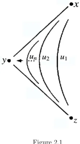
com-pactness of the moduli space. Unfortunately, ˆµx,y is not always compact. As a
counterexample, suppose there is a sequence {uˆn} ⊆µˆx,y sketched in Figure 2.1.
Figure 2.1
Then {uˆn} does not have a subsequence that is convergent in ˆµx,y (Consider
the example of M being a tilted torus andf being the height function). To solve this problem, we add some elements called broken flow line to ˆµx,y to compatify
the moduli space.
Definition 2.14. A sequence{uˆn} ⊆µˆx,y converges to (ˆv1, ...,vˆi)∈µˆx,y1×µˆy1,y2×
...×µˆyi−1,y if for any lift un of ˆun and vj of ˆvj, there are shiftsτn,j such that
un·τn,j Cloc∞
−−→vj ∀j ∈ {1, ..., i−1}
where y1, ..., yi−1 are critical points off.
Let
¯ ˆ
µx,y = ˆµx,y
G
( [
y1,...yi−1
ˆ
µx,y1 ×µˆy1,y2 ×...×µˆyi−1,y)
then we have the following proposition.
[image:36.595.193.333.200.452.2]2.5. COMPATIFICATION OF µˆX,Y 27
Lemma 2.16. Suppose{un} ⊆µx,y, then there exists a subsequence {unj} s.t.
unj
C∞
loc
−−→v
where v is also a gradient flow line.
Proof. We first show {un} is equicontinuous inC0(R, M). For all t1, t2 ∈Rwith t1 ≤t2
Z t2
t1
|u˙n(t)|2 dt=
Z t2
t1
hu˙n,− 5f◦unidt≤f(x)−f(y)
then
d(un(t1), un(t2)) ≤
Z t2
t1
|u˙n(t)|dt
≤
s
(t2−t1)
Z t2
t1
|u˙n(t)|2 dt (Holder inequality)
≤ p(t2−t1)(f(x)−f(y))
which implies the equicontinuity.
The compactness of M implies that un are uniformly bounded. By
Arzela-Ascoli theorem, there is a subsequence {unj} and v ∈C
0(
R, M) such that
v(t) = lim
j→∞unj(t) (∀t∈R) unj |[−R,R]
C0([−R,R])
−−−−−−→v |[−R,R] (∀R >0)
Since ˙un =− 5f ◦un and the gradient vector field of f is smooth, we have the
Ck-convergence
unj |[−R,R]
Ck([−R,R])
−−−−−−→ v |[−R,R] (∀R >0) with v˙ =− 5f ◦v
iteratively for all k∈N.
Lemma 2.17. Suppose{un} ⊆µx,y, v ∈µx,y and un Cloc∞
−−→v, then
un Px,y1,2
−−→v
Proof. First we prove un converge uniformly to x and y, i.e. for any
neighbour-hood Ux, Uy of x and y, ∃T >0 s.t. ∀n∈N
un(t)∈Ux (∀t <−T) un(t)∈Uy (∀t > T)
Suppose not, i.e. there exists Uy 3 y, tn → +∞ such that un(tn) ∈/ Uy.
Consider the Morse coordinate neary. Without loss of generality, assumeUy is a
ball centered atywith radius. Then for allp∈W(x, y), ifpis in the local chart ofy,x(p) = (0, ...,0, xλ+1, ..., xn), thenf(p)−f(y) =x2λ+1+...+x2n< ⇔p∈Uy.
If p is out of the local chart ofy, thenf(p)−f(y)≥. Therefore un(tn)∈/ Uy ⇒f(un(tn))−f(y)≥
Suppose f(v(to)) = 2 +f(y), then by making n large enough tn > t0, we have
f(un(t0))−f(y)≥f(un(tn))−f(y)≥
which contradicts un(t0)→v(t0).
Having the uniform convergence of un, along with the exponential decay we
have shown in lemma 2.5, we can say that there are , C, T > 0 such that for all n ∈N
d(un(t), x) ≤ Cet (∀t <−T)
d(un(t), y) ≤ Ce−t (∀t > T)
On (−∞,−T] and [T,+∞), the exponential convergence impliesH1,2-convergence.
On the comact set [−T, T], convergence in Cloc∞ impliesH1,2-convergence.
Proof. (of proposition 2.15)
For{un} ⊆µx,y, lemma 2.16 tells us there is a subsequenceunj
C∞loc
−−→v, where v is a gradient flow line. However the problem is v may not lie in µx,y. Suppose
v ∈µx0,y0, then f(v(R))⊆[f(y), f(x)] implies that f(y)≤f(y0)≤f(x0)≤f(x).
Now we discuss different cases of x0 and y0.
Case 1: x = x0, y = y0, then lemma 2.17 gives us H1,2-convergent subsequence
directly.
Case 2: x=x0,y6=y0. Choose a∈(f(y), f(y0)) anda is a regular value of f and a sequence of shifting {τj} such that
f(unj(τj)) =a
Denote ˜uj =unj·τj. Apply lemma 2.16 to{u˜j}, we have a subsequence such that
˜ ujk
Cloc∞
−−→˜v and f(y)≤f(˜v(+∞))≤f(˜v(−∞))≤f(y0).
Iterating these procedures finitely many times leads to the limit. We are immediately led to the conclusion:
2.6. GLUING 29
2.6
Gluing
We have shown that the space of flow lines ¯µˆx,y is compact and ˆµx,y is a manifold
of dimension ind(x)−ind(y)−1. Now we study what happened in the neigh-bourhood of the broken flow lines. This is described in the following so-called gluing theorem.
Theorem 2.19. Letx, y, z be critical points withind(x)> ind(y)> ind(z), given a compact set K ⊆µx,y×µy,z, there is a lower bound ρ0 >0 and a smooth map
]:K ×[ρ0,+∞)→µx,z
such that
1. ] induces a smooth embedding
ˆ]: ˆK ×[ρ0,+∞),→µˆx,z
2. As ρ→+∞, ˆ](ˆu,v, ρ)ˆ C
∞
loc
−−→(ˆu,vˆ)
3. If {ˆln} ⊆ µˆx,z converges to (ˆu,vˆ), then ˆln are in the range of ˆ] for
suffi-ciently large n.
The entire proof is rather complicated so we first give a brief outline of the proof. The construction of the gluing map is carried out in three steps:
(1) Establishing a “pre-gluing map”]0ρ, which glue broken flow lines (u, v) and end up with a smooth curve inPx,z1,2. This curve is an approximate solution of the negative gradient flow from x to z in the following sense: (u]0ρv)(R) differs fromu(R)∪v(R) by a sufficiently small amount and the convergence
(u]0ρv) C
∞
loc
−−→(ˆu,v)ˆ is provided asρ→+∞.
(2) Forming a procedure of associating nearby flow lines fromµx,z to those
pre-glued curves in a unique way for large ρ. We will construct a map, which is denoted by:
expωρ((γ(u, v, ρ)))
for someγ ∈H1,2(ω∗
ρT M) = TωρP
1,2
x,z whereωρ=u]0ρv. We will show it is a
real gradient flow line.
2.6.1
Pre-gluing
Throughout the whole section we choose two cut-off functionsβ± ∈C∞(R,[0,1]) such that
β−(t) =
1 t≤ −1 0 t≥0
and β+(t) =
0 t≤0 1 t≥1 which is shown schematically in the figure 2.2.
Figure 2.2 We define the pre-gluing map by
(u]0ρv)(t) =
uρ(t) t ≤ −1
expy(β−exp−y1(uρ) +β+exp−y1(v−ρ)) |t|≤1
v−ρ(t) t≥1
where uρ=u(·+ρ),v−ρ=v(· −ρ). Note that this formula makes sense only for |t |≤1,uρand v−ρare in the image of exponential. Fortunately, these conditions
are true for ρ large enough since lim
t→+∞u(t) =y= limt→−∞v(t). ωρ(=u]0ρv) has the following properties:
(1) ωρ∈Cx,z∞.
(2) ωρ(0) =y.
[image:40.595.80.480.178.729.2]2.6. GLUING 31
(4) ]0 is smooth.
(5) limρ→+∞ωρ(t) = y.
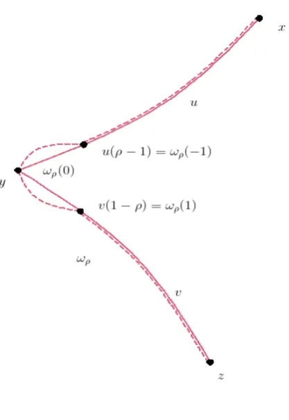
[image:41.595.188.397.234.537.2]Figure 2.3 sketches what happens:
Figure 2.3
We will also need the linearized version. First, we collect some background material. Let τ : T M → M denote the projection map, K : T T M → T M be the Levi-Civita connection map defined by the Riemannian metric g and exp :
O ⊆T M →M be the corresponding exponential map. As a consequence,K and Dτ : T T M →T M yield a decomposition of T T M into a horizontal bundle and a vertical bundle: Tξ,v(T M) = ker(Dτ(ξ)), Tξ,h(T M) = ker(K), ξ ∈ T M. We
then obtain two isomorphisms:
51exp(ξ) =Dexp(ξ)◦(Dτ |Tξ,h(T M))
−1 :T
τ(ξ)M
∼
=
−→Texp(ξ)M
52exp(ξ) = Dexp(ξ)◦(K |Tξ,v(T M))
−1 :T
τ(ξ)M
∼
=
We are able to define the linear version of the pre-gluing operation: Letξ ∈TuPx,y1,2
and η ∈TvPy,z1,2
(ξ]lρη)(t) =
ξρ(t) t≤ −1
52exp(β−52exp−1(ξρ) +β+52exp−1(η−ρ))(t) |t|≤1
η−ρ(t) t≥1
In the process of construction of the gluing map, we deduce the linearisation of the gluing map from the linear version of pre-gluing. By the linearisation of the actual gluing map we mean a projection onto the tangent bundle of µx,z as a
subbundle of H1,2.
Definition 2.20. Since Du = DFu and Dv = DFv are surjective Fredholm
operators,
(ker)2 = [
(u,v,ρ)
kerDu×kerDv ⊆(H1,2)2
is a subbundle with constant and finite dimension. Then we can define
L⊥(u,v,ρ)={vρ ∈H1,2(ωρ∗T M)| hvρ, ξ]lρηi0,2 = 0 f or all (ξ, η)∈kerDu×kerDv}
The importance of L⊥(u,v,ρ) lies in the following sense: one would like to glue the flow linesuand v in such a way to get a flow line fromxtoz. Now the result ωρ of the pre-gluing operation lies in Px,z1,2 but fail to be a flow line. However, by
perturbing ωρ with a small correction term γ ∈ L⊥(u,v,ρ) one does obtain a flow
line.
Sinceωρ ∈Px,z1,2, we can consider the local representation:
Fωρ =52exp
−1
ωρ ◦F ◦expωρ :Oωρ ⊆H
1,2(ω∗
ρT M)→L2(ω
∗
ρT M)
We also have the identity: Fωρ(0) =F(ωρ)(One can see [7,P74] for details of this
result).
The following results holds:
Proposition 2.21. ([7,Proposition 2.50]) If ρ0 is large enough, for any ρ > ρ0,
DFωρ(0) :H
1,2
(ω∗ρT M)→L2(ω∗ρT M) is surjective and the map
P rojρ◦]lρ:kerDFu×kerDFv
∼
=
−→kerDFωρ(0)
2.6. GLUING 33
Then from proposition 2.21,
kerD= [
(u,v)∈K,ρ≥ρ0
kerDFωρ(0)
is a vector bundle on K×[ρ0,∞) with dimension ind(x)−ind(z) and
L⊥ = [
(u,v)∈K,ρ≥ρ0
L⊥(u,v,ρ)
is finite-codimensional bundle such that kerDFωρ(0)⊕L
⊥
(u,v,ρ)=H1,2(ω
∗
ρT M)
Hence
DFωρ(0)|L⊥(u,v,ρ):L
⊥
(u,v,ρ) →L 2
(ωρ∗T M) is bijective and we denote the inverse map by
Gωρ = (DFωρ(0)|L⊥(u,v,ρ))
−1
:L2(ω∗ρT M)−→∼= L⊥(u,v,ρ)
2.6.2
The construction of gluing map
]
Given the pre-gluing map ]0, which is an approximate version of the gluing
op-eration, we now try to find a correction term for ]0 using the normal bundle L⊥ constructed above. In other words, we want to find a section γ ofH1,2(P1,2∗
x,z T M)
over K×[ρ0,∞) so that
ψ(ρ) =expωρ((γ(u, v, ρ)))
is a real gradient flow line. Therefore we need the section γ :K ×[ρ0,∞)→H1,2(Px,z1,2∗T M)
satisfies F ◦γ = 0. Besides, we want expωρ((γ(u, v, ρ))) converge to the broken
flow lines (u, v) as ρtends to infinity. From the previous section we can see that the convergence property holds for pre-gluing map, so the correction term should converges to zero, i.e. γ(u, v, ρ)→0 as ρ→ ∞.
Now we introduce a basic analytic machinery of this section.
Lemma 2.22. Let X and Y be two Banach spaces and f :X →Y be a smooth map of the form
(1) Df(0)◦G=Id.
(2) There exists a constant C >0 such that the contraction property
kGN(x)−GN(y)k≤C(kxk+kyk)kx−yk
holds for all x, y in B(0), where = 51C.
(3) kGf(0)k≤
2.
Then there exists a unique α ∈ Im(G)∩B(0) such that f(α) = 0. Moreover, kα k≤2kGf(0)k.
Proof. We prove this lemma using the contraction mapping principle. Define φ :X→X by setting
φ(x) = G(Df(0)x−f(x)) =−G(f(0) +N(x))
We first show that x is a zero point of f if and only if φ(x) =x. Note that Df(0)φ(x) = Df(0)G(Df(0)x−f(x)) =Df(0)x−f(x)
Hence φ(x) =x implies f(x) = 0. Conversely, if f(x) = 0 and x=G(y), then φ(x) = GDf(0)(x) = GDf(0)G(y) =G(y) =x
We will therefor show thatφ has a unique fixed point inB(0).
First,φ sends B(0) to itself: Ifkxk≤, then
kφ(x)k=kG(f(0) +N(x))k ≤ kGf(0)k+kGN(x)k
≤
2 +C kxk
2 (sinceN(0) = 0)
≤
2 +C
2
= 2+
5 < Next, if x and y are two points of B(0), then
kφ(x)−φ(y)k=kGN(x)−GN(y)k ≤ C(kxk+kyk)kx−y k ≤ 2Ckx−yk= 2
5 kx−yk By the contraction mapping theorem, there is a unique α ∈ B(0) satisfying
2.6. GLUING 35
It remains to show the inequality stated in the lemma. We have
kαk − kφ(0) k≤kφ(α)−φ(0) k≤ 2
5 kαk≤ 1 2 kα k It follows that
kα k≤2kφ(0)k= 2 kGf(0)k.
We are going to apply lemma 2.22 on Fωρ =52exp
−1
ωρ ◦F ◦expωρ :H
1,2(ω∗
ρT M)→L2(ω
∗
ρT M)
which can be express explicitly as
Fωρ(x) =5tx+ Θ(x)·ω˙ρ+52exp
−1
ωρ ◦ 5f◦expωρ
where Θ(x) = (52exp(x))−1 ◦ 51exp(x) : Tτ(ξ)M
∼
=
−→ Tτ(ξ)M. Consider the
ex-pansion of Fωρ as the form of the formula of lemma 2.22:
Fωρ(x) = Fωρ(0) +DFωρ(0)·x+Nωρ(0, x)
Compute the difference of the nonlinear term at two different points: Nωρ(x)−Nωρ(y) = Fωρ(x)−Fωρ(y)−DFωρ(0)·(x−y)
= DFωρ(y)(x−y) +Nωρ(y, x−y)−DFωρ(0)·(x−y)
= (DFωρ(y)−DFωρ(0))·(x−y) +Nωρ(y, x−y)
Since K is compact, we have the following estimate for some constantC:
kNωρ(x)−Nωρ(y)k0,2≤C(kxk1,2 +kyk1,2)kx−yk1,2 (2.5)
To get the required estimate in lemma 2.22, we need the following lemma. Lemma 2.23. ([7,lemma 2.51]) If ρ0 is large enough, there exists a constant
C > 0 such that the isomorphism Gωρ satisfies
kGωρξk1,2≤C kξk0,2 ∀ρ∈[ρ0,∞), ξ ∈L
2(ω∗
ρT M)
Then (2.5) together with lemma 2.23 implies that there exists a constant C > 0 such that
kGωρNωρ(x)−GωρNωρ(y)k1,2 ≤ C(kxk1,2 +kyk1,2)kx−yk1,2
for all (u, v, ρ)∈K×[ρ0,∞).
Now, in order to apply lemma 2.22, it remains to show thatkF(ωρ)k0,2 tends
to zero as ρ goes to infinity. This result follows from the next lemma. Lemma 2.24. There are constants c, δ >0 such that
kF(ωρ)k0,2≤ce−δρ
for all (u, v, ρ)∈K×[ρ0,∞).
Proof. By the definition of ]0, we have the identity:
F(ωρ)(t) = 0 f or |t|>1
So, without loss of generality,
u(t) = expyξ(t) t≤ −ρ−1
v(t) = expyη(t) t ≥ρ+ 1
Consider the local coordinates near y, F = ∂t∂ +X : H1,2(R,Rn) → L2(R,Rn), where X :R→Rn and DX(0) is the Hessian of f aty. Then we have
ωρ =β−·ξρ+β+η−ρ
Hence
kF(ωρ)kL2 = kF(ωρ)kL2([−1,1])≤constkωρkH1,2([−1,1])
≤ const(kξρ kH1,2([−1,0]) +kη−ρkH1,2([0,1]))
Since ξ and η satisfy exponential decay at the critical point 0:
|ξ(t)|≤const e−δt and |η(−t)|≤const e−δt f or t ≥0
The constant δ depends only on the Hessian of f at y, and we can make c independent of ξ and η by compactness of K. Since
kξρ kH1,2([−1,0])≤ sup
t∈[−1,0]
{|ξ(t+ρ)|} ≤const e−δρ
Similarly, kη−ρkH1,2([0,1])≤const e−δρ. These complete the proof.
Up to now, we haveFωρ :H
1,2(ω∗
ρT M)→L2(ω
∗
ρT M) andGωρ :L
2(ω∗
ρT M)
∼
=
−→
L⊥(u,v,ρ) ⊆ H1,2(ω∗
2.6. GLUING 37
conclude that there exists a unique correction term γ(u, v, ρ) ∈ B(0) ∩L⊥(u,v,ρ)
such that
Fωρ(γ(u, v, ρ)) = 0
and
kγ(u, v, ρ)k1,2 ≤ 2kGωρFωρ(0)k1,2
≤ 2C kFωρ(0) k0,2= 2C kF(ωρ)k0,2
Hence
kγ(u, v, ρ)k1,2<2cCe−δρ
which verifies the assertion we made at the beginning of the section(γ(u, v, ρ)→0 asρ→ ∞). And the smoothness of γ follows from the implicit function together with the smoothness of F.
Now we have finished the definition of the gluing map
]:K×[ρ0,∞) → µx,z
(u, v, ρ) 7→ expωργ(u, v, ρ)
The following two propositions that states the embedding property and the last two assertions in theorem 2.19 help us finish the proof of theorem 2.19. Proposition 2.25. If ρ0 is large enough, the unparametrized gluing map
ˆ]: ˆK×(ρ0,∞) → µˆx,z (ˆu,ˆv, ρ) 7→ u]ˆ ρvˆ
is a smooth embedding.
Proposition 2.26. Suppose (ˆu,vˆ) ∈ µˆx,y ×µˆy,z, and {ρn} is an increasing
se-quence tends to infinity. then
ˆ uˆ]ρnvˆ
Cloc∞
−−→(ˆu,v)ˆ
And the converse is also true, that is, any sequence of unparametrized flow line converging to (ˆu,v)ˆ finally lies in the range of ˆ].
2.6.3
Conclusion
We have stated and proved the gluing theorem under general condition, in fact, we only need to consider broken flow lines with one break and the relative Morse index ind(x)−ind(z) = 2, which is sufficient to construct the Morse complex. Since the space of broken flow lines appears as a compatification of the space of flow lines, the space of flow lines ¯µˆx,z is compact and ˆµx,z is a manifold of
dimension 1. After study about what happens in the neighbourhood of broken flow lines, we have the following theorem.
Theorem 2.27. Let x and z be two critical points with relative index equals to 2, then µ¯ˆx,z is a compact manifold of dimension 1 with boundary and
∂µ¯ˆx,z =
[
ind(x)=ind(y)+1
ˆ
µx,y×µˆy,z
Hence we are able to classify the component of ˆµx,z by two types: one is
diffeomorphic to S1 and the other one is diffeomorphic to an open interval. For
the latter type, there are exactly two different broken flow lines as its boundary.
2.7
Orientation
In section 2.5 we have shown that ˆµx,y is consist of finitely many unparametrised
flow lines when the relative index ofxandyis one. The definition of the boundary operator∂ in Morse-Smale complex requires us to count the elements in ˆµx,y with
sign. These signs are determined by the orientation of the ˆµx,y and ˆu∈µˆx,y. The
orientation of ˆuis the canonical orientation of the flow line. So we need to define a coherent orientation for the moduli space.
2.7.1
The determinant line bundle
Consider two finite dimensional real vector spaces E, F. We define a one-dimensional vector space by
Det(E, F) = (∧maxE)O(∧maxF)∗ where ∧maxE =∧dimEE and ∧0E =
R for any E.
Lemma 2.28. Given an exact sequence of finite-dimensional real vector spaces 0→E1
d1
−→E2
d2
2.7. ORIENTATION 39
There exists a canonical isomorphism
φ: O
i even
(∧maxE i)
∼
=
−→ O
i odd
(∧maxE i)
Proof. Suppose e11, ..., e1n1 is a basis ofE1. By the exactness of the sequence, d1
is injective, so we can extend the linear independent vectors d1(e11), ..., d1(e1n1)
to a basis of E2, suppose is d1(e11), ..., d1(e1n1), e21, ..., e2n2.
Claim: d2(e21), ..., d2(e2n2) are linearly independent in E3.
Suppose not, then x1d2(e21) +...+xn2d2(e2n2) = 0 for some x1, ..., xn2 ∈ R
with x1·...·xn2 6= 0. Hence
x1e21+...+xn2e2n2 ∈ker(d2) =Im(d1)
⇒ x1e21+...+xn2e2n2 =y1d1(e11) +...+yn1d1(e1n1)
⇒ x1 =...=xn2 =y1 =...=yn1 = 0
It is a contradiction.
Then we can extendd2(e21), ..., d2(e2n2) to a basis ofE3, say,d2(e21), ..., d2(e2n2), e31, ..., e3n3.
Similarly, for each 1< i≤k−1, we can find a basis of Ei+1 of the form
di(ei1), ..., di(eini), ei+1 1, ..., ei+1 ni+1
where nk = 0 since dk is surjective. Then we defineφ by
(d1(e11)∧...∧d1(e1n1)∧e21...∧e2n2 ⊗...)
7→ (e11∧...∧e1n1 ⊗d2(e21)∧...∧d2(e2n2)∧...)
This map is independent of the choice of the bases of the vector spaces, since any change of bases operates by multiplication with same determinant of the transformation on both sides of φ.
Suppose now X is a topological space and f :X →F(H0, H1)
be a continuous map, whereH0,H1are Banach spaces. We define the determinant
of a Fredholm operator F as
Det(F) :=Det(kerF, cokerF) Besides, we define
Det(f) := [
x∈X
Ifdim(ker(f(x))) is locally constant, since Fredholm index is locally constant, so is dim(coker(f(x))). Then ker(f) := S
x∈X{x} ×kerf(x) and coker(f) :=
S
x∈X{x} ×cokerf(x) can be seen as sub-bundles ofX×H0 andX×H1
respec-tively overX. Therefore we haveDet(f) =∧maxker(f)⊗(∧maxcoker(f))∗, which implies that Det(f) is a real line bundle. However, without the assumption, we still have the property.
Proposition 2.29. Det(f) = S
x∈X{x} ×Det(f(x))→X is a real line bundle.
Proof. The proof follows from [4, Appendix]. Let ψ : Rn → H
1 be a linear map such that ˆfψ(x) is a surjective Fredhom
operator for some x∈X, where ˆfψ is defined as
ˆ
fψ :X → L(Rn×H0, H1)
x 7→ ((h, k)7→ψ(h) +f(x)k)
Then we can find an open neighbourhood U(x)3x such that ˆfψ(y) is surjective
for ally ∈U(x) and the Fredholm index of ˆfψ(y) constantly equals toind( ˆfψ(x))
on U(x). Hence we define fψ(y) fory∈U(x) as follows:
fψ(y) :Rn×H0 → Rn×H1
(h, k) 7→ (0,fˆψ(y)(h, k))
Therefore dim(kerfψ(y)) and dim(cokerfψ(y)) are constant on U(x). Thus, we
have a determinant bundle
Det(fψ) πψ
−→U(x)
as long as (x, ψ, U(x)) satisfies conditions described above. Consider the exact sequence fory∈U(x):
0→kerf(y) d1
−→kerfψ(y) d2
−→Rn d3
−→cokerf(y)→0
defined by
d1(k) = (0, k)
d2(h, k) = h
d3(h) = [ψ(h)]R(f(y))
According to lemma 2.28, we have a canonical isomorphism φy,ψ:∧maxker(f(y))⊗ ∧maxRn
∼
=
−→ ∧maxker(f
2.7. ORIENTATION 41
Tensor both side ofφy,ψ by (∧maxRn)∗⊗(∧max(cokerf(y))∗). Since for all finite-dimensional real vector spaceE, (∧maxE)⊗(∧maxE)∗ ∼
=R via the mapξ⊗η∗ 7→
η∗(ξ). We obtain an isomorphism:
Det(f(y))−→ ∧∼= maxker(fψ(y))⊗(∧maxRn)∗ =Det(fψ(y))
The equality comes from the identity cokerfψ(y) = (H1 ×Rn)/H1× {0} =Rn.
Then we have isomorphisms on fibres of Det(fψ) andDet(f)|U(x):
Det(fψ)
∼
=//
πψ
Det(f)|U(x)
π
ww
pppppp ppppp
U(x)
It remains to show that for two admissible triples (x, ψ, U(x)) and (x0, ψ0, U(x0)), the transition map
Det(fψ)|V
transition
−−−−−−→Det(fψ0)|V
is a vector bundle isomorphism, where V =U(x)∩U(x0). Assume ψ0 :Rn0 →H
1, we define
ψ⊕ψ0 :Rn×Rn0 → H
1
(h, k) 7→ ψ(h) +ψ0(k) Then for y∈V, we have an exact sequence
0→kerfψ(y)→kerfψ⊕ψ0(y)→Rn 0
→cokerfψ(y)→0
By similar calculation as before, we obtain an isomorphism Det(fψ(y))
∼
=
−→Det(fψ⊕ψ0(y))
Then it is obvious that Det(fψ)
∼
=
−→ Det(fψ⊕ψ0) is a vector bundle isomorphism
over V. We have the same result for Det(fψ0⊕ψ). And we can easily induce
a vector bundle isomorphism Det(fψ⊕ψ0 → Det(fψ0⊕ψ) from the vector
bun-dle isomophisms between kernel and cokernel bunbun-dles of the type (h1, h2, k) 7→
(h2, h1, k). Then the results follows from the commutative diagram:
Det(fψ)transition//
∼
=
Det(fψ0)
∼
=
Det(fψ⊕ψ0
∼
= //
Det(fψ0⊕ψ)
Definition 2.30. An orientation of a family of Fredholm operators f : X →
2.7.2
Orientation on glued Fredholm operators
Let A be an element in C( ¯R, End(Rn)) such that A± =A(±∞)∈ GL(n,
R) are nondegenerate self-adjoint operators on Rn. Then we define a set of special class
of Fredholm operators: Θ(A−, A+) ={d
dt +A|A∈C( ¯R, End(R
n)), A±
=A(±∞)}
Elements in Θ(A−, A+) are Fredholm operators defined fromH1,2(R,Rn) toL2(R,Rn). And we also have the following index property:
ind(F) = ]{negative eigenvalue of A−} −]{negative eigenvalue of A+} (2.6) We also have the following property for Θ(A−, A+):
Proposition 2.31. ([7, lemma 2,15]) Θ(A−, A+) is contractible in Σ =S
Θ(M1, M2), where M1, M2 are
nondegen-erate self-adjoint operators on Rn.
Suppose K = dtd +A∈Θ(A−, A+) and L= dtd +B ∈Θ(B−, B+) are asymp-totically constant operators, i.e.
A(t) =
A− t≤ −T
A+ t≥T and B(t) =
B− t ≤ −T B+ t ≥T
Definition 2.32. The gluing operation for asymptotically constant operators K, L with A+ =B− is defined by
K]ρL=
d
dt +C ∈Θ(A −
, B+) where
C(t) =
A(t+ρ) t≤0 B(t−ρ) t ≥0 for all ρ≥T.
From (2.6), we have the following fomula
ind(K]ρL) =ind(K) +ind(L)
Now, the crucial question is whether there is a concept of orientation of K]ρL