Differential Evolution with an Evolution Path:
A DEEP Evolutionary Algorithm
Yuan-Long Li, Student Member, IEEE, Zhi-Hui Zhan, Member, IEEE, Yue-Jiao Gong, Student Member, IEEE,
Wei-Neng Chen, Member, IEEE, Jun Zhang, Senior Member, IEEE, and Yun Li, Member, IEEE
Abstract—Utilizing cumulative correlation information already existing in an evolutionary process, this paper proposes a predic-tive approach to the reproduction mechanism of new individuals for differential evolution (DE) algorithms. DE uses a distributed model (DM) to generate new individuals, which is relatively explorative, whilst evolution strategy (ES) uses a centralized model (CM) to generate offspring, which through adaptation retains a convergence momentum. This paper adopts a key fea-ture in the CM of a covariance matrix adaptation ES, the cumulatively learned evolution path (EP), to formulate a new evolutionary algorithm (EA) framework, termed DEEP, stand-ing for DE with an EP. Without mechanistically combinstand-ing two CM and DM based algorithms together, the DEEP frame-work offers advantages of both a DM and a CM and hence substantially enhances performance. Under this architecture, a self-adaptation mechanism can be built inherently in a DEEP algorithm, easing the task of predetermining algorithm control parameters. Two DEEP variants are developed and illustrated in the paper. Experiments on the CEC’13 test suites and two practical problems demonstrate that the DEEP algorithms offer promising results, compared with the original DEs and other relevant state-of-the-art EAs.
Index Terms—Cumulative learning, differential evolution (DE), evolution path (EP), evolutionary computation.
I. INTRODUCTION
I
N EVOLUTIONARY algorithms (EAs), two types of mod-els are often used to generate new candidate solutions, which we refer to as a distributed model (DM) and a cen-tralized model (CM) in this paper. For example, in the genetic algorithm (GA) [1], differential evolution (DE) [2], and parti-cle swarm optimization (PSO) [3]–[9], each new candidate isManuscript received March 10, 2014; revised June 29, 2014; accepted September 16, 2014. Date of publication October 9, 2014; date of current version August 14, 2015. This work was supported in part by the National High-Technology Research and Development Program (863 Program) of China under Grant 2013AA01A212, in part by the National Natural Science Foundation of China (NSFC) under Grant 61402545 and Grant 61379061, in part by the NSFC Key Program under Grant 61332002, and in part by the NSFC for Distinguished Young Scholars under Grant 61125205. This paper was recommended by Associate Editor P. N. Suganthan.
Y.-L. Li, Z.-H. Zhan, Y.-J. Gong, W.-N. Chen, and J. Zhang are with Sun Yat-sen University, Guangzhou 510275, China, also with the Key Laboratory of Machine Intelligence and Advanced Computing, Ministry of Education, Guangzhou 510275, China, also with the Engineering Research Center of Supercomputing Engineering Software, Ministry of Education, Guangzhou 510275, China, and also with the Key Laboratory of Software Technology, Education Department of Guangdong Province, Guangzhou 510275, China (e-mail:[email protected]).
Y. Li is with the School of Engineering, University of Glasgow, Glasgow G12 8LT, U.K.
Color versions of one or more of the figures in this paper are available online athttp://ieeexplore.ieee.org.
Digital Object Identifier 10.1109/TCYB.2014.2360752
evolved from certain parental individuals directly. This can be regarded as following a DM because the parents are distributed among the population. On contrast, in evolution strategy (ES) algorithms, such as the estimation of distribution algorithm (EDA) [10] and the covariance matrix adaptation ES (CMA-ES) [11], all new individuals are generated using a centralized probability model. Similarly, in ant colony opti-mization (ACO) [12], [13], all ants use the same pheromone model to generate new individuals. Therefore, these algorithms can be regarded as using a CM to generate new candidates because the parental information is centralized with an inter-mediate model. Note that some other classification terms, such as explorative/exploitative, diversification/intensification, and individual-based/model-based, can also be used in classifying EAs from different perspectives. The term DM/CM is used in this paper because this paper focuses on the features of how parental information is utilized in the evolutionary process.
In this paper, we first analyse the different features and advantages of a DM and a CM, with a focus on combining their advantages in the development of new algorithms. In the literature, efforts are already seen in combining a CM with a DM [14]–[19]. In [14], for example, the use of some DM features to enhance the ACO algorithm is proposed, which shows some promising results. In [20], the teaching–learning optimization proposal combines a CM (a “teacher phase”) and a DM (a “learner phase”) for constrained optimization. Other relevant studies have focused on using a DM as a base algo-rithm, such as the combinations of DE and EDA [17], [19], PSO and EDA [15], and DE and CMA-ES [21]. These are however, based on a direct combination of two algorithms of a DM and of a CM. Hence, new populations are generated in both ways to introduce and maintain a higher diversity than using a single model alone.
However, such hybridizations result in complex reproduction processes and lack the advantage of efficient cumulative learning offered by a CM, such as the evolution path (EP) used in a CMA-ES. This paper therefore attempts to address these issues by developing a “DE with an EP” (DEEP) algorithm, using DE as the base algorithm with enhancement through an EP.
The remainder of this paper is organized as follows. In Section II, the DM and CM are fully analyzed, with reviews on several related search models. In Section III, the DEEP framework is introduced. In Section IV, two DEEP algorithms are developed and experiments on the CEC’13 test suites are performed to test the DEEP algorithms fully. The conclusion is drawn in Section V, with future work also highlighted.
Fig. 1. Two kinds of population reproduction models: DE versus EDA.
II. REPRODUCTIONMODELS
This section analyses the differences and advantages of the DM and CM models in generating new individuals. Take DE and EDA as examples for the use of DM and CM, respectively. Their differences are illustrated in Fig. 1.
Firstly, each new individual in the DE is generated based on its own parents. In this sense, different new individuals can be regarded to be generated according to the different mod-els determined by their corresponding parental individuals. Therefore, the whole population in DE can be regarded as gen-erated by combining multiple models. However, in an EDA, a uniform reproduction model is first created by using the information from some selected parents, and then the whole population is generated from a uniform Gaussian model. From this viewpoint, the DE reproduction model is regarded as a DM while the EDA a CM.
[image:2.612.315.558.56.226.2]Secondly, in DE, the new population is directly generated by the parent population while in EDA the population is first built into a Gaussian model, which is then used as an intermediary parametric model to generate the new population. Therefore, a DM in DE is nonparametric whilst a CM in EDA is parametric. Moreover, these two different types of models have different advantages. The DM scheme enjoys flexibility in nonparamet-ric modeling and distributed individual generation. There is a direct generational parent-offspring relationship between the two successive generations. New individuals can be gener-ated alongside the best parental individuals regardless of their distribution. On the other hand, as the CM scheme builds a Gaussian model as an intermediate model to generate new individuals, the CM scheme usually cannot work well on multimodal problems when the population is separately dis-tributed in different locales. However, the CM scheme enjoys its advantage of parametric modeling, which can cumulate historical information continuously during the evolutionary process. The continuous adaptation of the CM can help adjust the shape and location of the Gaussian model to gain a better landscape approximation. Compared with the contin-uously learning feature of the CM, the DM scheme can only use the information of the immediate past generation, which is regarded as “discrete” in such a sense. Therefore, the
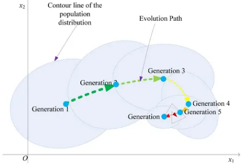
Fig. 2. Evolution path over a number of generations.
advantage in cumulative learning helps algorithms with a CM (such as the CMA-ES) work better on ill-shaped landscapes such as nonconvex or narrow corridor ones [11].
Given the analysis above, a question arises whether the advantages of both kinds of models can be combined. In the lit-erature, some studies are reported in the sense of this question. Deb et al. [22] and Someya [23] assert that there are different kinds of crossover mechanisms in GA, such as the “parent mode crossover,” with which each offspring is generated by a corresponding parent, while “centric mode crossover” opera-tions generate the whole offspring population by the center of the current population. Someya [23] proposes an asymmetric normal distribution crossover (ANDX) operation to tune these two crossover modes for improved performance. For ACO, Tsutsui [14] provides an interesting way to use the parental solutions to modify new solutions generated by the CM model with promising results.
Based on the analysis so far, we propose a new way other than direct combination of a DM and a CM. Here, the main structure of one model is retained while key features of the other are added to keep the hybridized algorithm as simple as possible. In this paper, we use the DE (which is based on a DM) as the base algorithm and combine some key features of a CMA-ES (which is based on a CM) into the DE framework. The cumulatively learned evolution path (EP) is used to adapt the parametric model of the CMA-ES for improved efficiency and performance. According to [11], the EP in the CMA-ES represents the migration path of the popu-lation center. Using EP to cumulatively modify the distribution shape of the Gaussian model plays a key role in the CMA-ES. As an illustration, Fig. 2 shows how the population center migrates, i.e., the EP.
However, sometimes the EP may detour from a specific center, like illustrated by the last several generations in Fig.2. Nevertheless, the center of the detoured EP may indi-cate a good region for generating a new promising solution. Therefore, an anchor point which is a weighted mean of the recent population centers is used to maintain some momentum of the EP when it detours significantly. This way, the algorithm can be guided by both the EP direction and the anchor points. Based on the analysis, it is apparent that the proposed DEEP scheme can be applied to more than one DE variant. In this paper, we illustrate and develop two DEEP algorithms, which are based on the conventional DE/rand variant and the well-performed adaptive DE variant, termed as JADE in [24]. In the remainder of this section, a brief review on DE and CMA-ES, which belong to DM and CM, respectively, are presented, along with a state-of-the-art DE/CMA-ES hybrid algorithm.
A. Models in DE
The DE algorithm is a typical EC algorithm with three basic operations for the population reproduction: mutation, crossover, and selection. In every generation, a population P first goes through mutation. The mutation operation of DE is very special in that it uses a linear combination of a base vec-tor and one differential vecvec-tor or more to generate a mutated vector. For example, for every individual xi (i = 1, . . . , population_size) in P, its mutated vector vi is generated by
vi=xr1 +F·
xr2−xr3
(1)
where r1, r2, and r3are three randomly selected individuals,
and are also different from i. In this mutation scheme, the dif-ference between individuals r2and r3is used as the mutation
step while factor F controls the step scale. After a mutated population V is created, it will go through a crossover process with the parent population P. The crossover operation for DE can be in binary or exponential. Here, without loss of gen-erality, we only illustrate the binary crossover, as it is used in most cases. The crossover operation recombines every pair of individuals of (vi, xi) to generate a new individual ui as shown in
uij=
vij,if rand(0,1)≤CR||j==jrand
xij,otherwise , for j=1, . . . ,D (2)
where rand(0,1) is a random number uniformly distributed within interval [0, 1], D is the number of dimensions, CR is the crossover rate which controls how many dimensions of the newly generated individual are from the mutated vector vi, and jrand is a randomly selected index to make sure that at least 1-D of the mutated vector will enter into the newly generated individual.
The crossover process creates a temporary population U, which is evaluated and then enters into the selection proce-dure. This procedure uses a pair-wise comparison of U and P. As shown in the following equation, individual ui and xi are compared and the better one will enter into the next generation:
xnewi =
xi,if fitness(xi)is better than fitness(ui)
ui,otherwise. (3)
The above basic framework of DE shows a very simple algo-rithm for continuous optimization problems. A recent survey on DE can be found in [25]. Recent studies on parameter adaptation [26]–[29] and parameter composition [30] have shown that algorithm parameters of DE are important for the DE to perform well on different kinds of problems. This observation has led to the use of different mutation strate-gies to improve the performance of DE [26], [27], [30]–[32]. Mallipeddi and Suganthan [33] have proposed the framework of using ensemble-based strategies and parameters. Resultant ensemble-based algorithms are shown to adaptively choose better performing strategies and parameters in dealing with various kinds of problems. In [34], a bare-bone algorithm is proposed to solve parameter setting problem. Moreover, mul-tiple or different individuals are used to guide the search of DE in [24] and [35]–[37], while local or neighbor informa-tion is used to guide the search in [38]–[41]. Both methods are used to improve the efficiency while maintaining the global search ability of DE. Recently, theoretical study on the convergence characteristics of DE has also made impor-tant progress in [42]. DE based frameworks are also proposed for constrained optimization in [43] and dynamic optimization in [44] and [45]. Multistart JADE is proposed in [46], which as a restart method works well for CMA-ES and EDA [47] and could be further extended to other evolutionary computation methods such as DE. In [48], a DE is reported to offer effi-cient solutions to multimodal optimization problems. Overall, current DE studies mainly cover ensemble-based algorithms, which have shown advantage with automatic strategies and parameter settings; parameter adaptation methods, which are important to DE algorithm to solve different kinds of prob-lems; and multiple guidance and local guidance, which have been shown very useful in improving the global search ability of DE. However, there has been no clear EP based studies for DE so far.
B. CMA-ES
The CMA-ES has proved to be one of the most promis-ing EAs. The CMA-ES uses CMA to adapt the Gaussian distribution model to generate new individuals, the same as in a common EDA. In CMA-ES, a covariance matrix C rep-resents the population distribution shape and is cumulatively updated.
Usually, there two ways to update the covariance matrix C, but test results reveals that the algorithm works well when C is updated by the “EP” only. The EP vEP is defined as the
cumulative migration step of the mean point of the population (xg−xg−1) between successive generations. The EP vector vEP can modify the shape of the distribution and enlarge it
along the direction of vEP by modifying C. CMA-ES works
C. DCMA-EA
In [21], a hybrid algorithm of DE and CMA-ES, termed differential covariance matrix adaptation EA (DCMA-EA), is proposed. The DCMA-ES combines the DE operations into the CMA-ES new individual generation, which is aimed to enhance the global search ability of CMA-ES. The DCMA-EA improves the performance of CMA-ES on complex multi-modal functions, but may not be efficient on some unimulti-modal or simple multimodal problems. The DCMA-EA uses the CMA-ES algorithm as a base algorithm. It thus inherits all the complex parameters and computations such as eigen-decomposition used in CMA-ES. Hence, it is more complex than traditional DE variants.
III. DEEP FRAMEWORK
Following the analysis of key features in the DE and CMA-ES algorithms, one key feature is selected in this section to improve DE without needing eigen-decomposition or direct hybridization of DE and CMA-ES. This is to retain simplicity in implementation and to improve efficiency in operation.
A. Concepts, Problems, and Solutions of DEEP
The principle of DEEP is to use the EP learning model of CMA-ES to enhance the DE reproduction. In particular, DEEP incorporates an EP vector in the mutation of the original DE algorithm. The EP is computed by accumulating historical information of the population migration as an intermediate CM for the DE to predict direction and hence move faster toward a more promising region.
In developing the DEEP algorithm, the first issue to address is to assess whether or not the population has already gone too far in the EP direction and whether the population need to reverse the direction. Our solution to this problem is to use an adaptive parameter α to control the direction (either positive for forward or negative for backward) of the mutation and its step size. Parameter α thus lets the program decide the direction and step size.
The second issue is to decide whether the direction of the EP makes sense when the EP detours significantly. Observation reveals that the EP often detours round and round when the population is around a best region and slowly converges to the approximate center. Hence we can use the historical centers of the recent populations to calculate the centroid of their recent trajectory (i.e., an approximate center of the recent evolution path). The centroid can therefore be used as an anchor point cEP to counter random detours.
B. Major Operations
Without loss of generality, EP is directly used as an addi-tional mutation vector in DEEP rather than as a means of building a covariance matrix used in CMA-ES. This way, the framework of DEEP remains unchanged from the original DE algorithm.
At the beginning, a normal DE population is generated. For every subsequent generation in the evolution process, each individual in the generation goes through the DE mutation and
crossover operations as shown in (1) and (2). Then an addi-tional EP mutation is added to the new individual ui(for i=1, . . . , population_size)
ui=ui+F·sCR·(αi·vEP+βi·(cEP−ui)) (4) where F and sCR = CR are the same parameters as F and CR in (1) and (2), vEP is the cumulative learning EP vector
and cEP is the anchor point. Parameter αi is generated with a Gaussian distribution to control the size and direction of EP and βi is a parameter used to control the step size to the anchor point cEP.
Based on (4), ui is further guided by the EP directional information and the anchor point. It should be noted that vEP is a vector along the population’s promising EP direction
and is therefore directly added to ui, while cEP advocates a
promising position with theβi–weighted difference (cEP – ui)
“correcting” ui.
The vEP vector is the migration vector of the mean point
of the population Centerg from the previous generation to the current generation g
vEP=Centerg−Centerg−1 (5)
where Centerg is the mean position of the first s best individ-uals in the population in generation g, defined as
Centerg=meanxbest_1,xbest_2, . . . ,xbest_s
. (6)
The anchor point cEPof the cumulative learning is defined as
cEP =λ·cEP+(1−λ)·Centerg. (7)
Based on (5) and (7), vEP and cEP collect the EP
infor-mation from two different aspects. Firstly, vEP is for a fast
response to the recent population migration vector, which can be very helpful when a long range migration is needed. Secondly, cEP is updated using a learning parameterλ, which
can be taken as a weighted mean of the recent population centers. This is useful when the population experience a con-traction process. Aλ value of 0.5 appears to be consistently good based on our experimental studies (Section IV). For the control parameters αi and βi in (4), simple self-adaptation suffices.
With the EP applied to new individuals, DEEP reproduction benefits from advantages of both distributed and CMs. In par-ticular, each individual inherits from its parents by (1) and (2), hence maintaining population diversity and good sampling of the search space. Then, (4) acts as a CM to track the best par-ents’ moving direction in the generation of new individuals. Fig.3 illustrates how a DEEP mutant is generated.
C. Parameter Adaptation in DEEP
Fig. 3. DEEP generates a new individual by adding vEP and a step
toward cEP.
Parameters αi and βi are self-adaptive in the algorithm. Parameter αi is generated with a Gaussian distribution, where both the size and sign of αi are used
αi=2N
αm, αsig
. (8)
The distribution is centered at αm, which creates a balance factor for the EP mutation direction. If αm > 0, the distri-bution gears toward the forward direction of vEP. If αm <0, the distribution gears toward the backward direction of vEP.
Parameter αm is adaptively adjusted in a way similar to how CR adapts in JADE [24]. Because N(αm,αsig)∈(−∞,∞),αi is truncated into an interval [−αmax,αmax] in implementations, as shown in
αi =
αmax, if αi> αmax
−αmax,if αi<−αmax. (9) After the evaluation of the population, those αi values that have helped generate better offspring are used to tune αm adaptively by way of
αm =0.9 αm+0.1 mean
αgood/2 (10) where mean (αgood) is the mean value of αi that have helped the individuals generate better new individuals. The momentum from αgoodhelps the algorithm adapt itself in the distribution of the EP during the search process.
Similarly, a self-adaptive adjustment for the scale factorβm is formulated. For each individual, βi is generated by
βi=
⎧ ⎨ ⎩
0,
βmax, ififββii<> βmax0 Nβm, βsig
, otherwise
(11)
where βm and βsig are the center point and standard devia-tion of the Gaussian distribudevia-tion used to generateβi. Thoseβi values,βgood, that have helped the individuals generate better new individuals are used for an adaptive center of the Gaussian distribution, as shown in
βm=0.9βm+0.1 mean
βgood. (12)
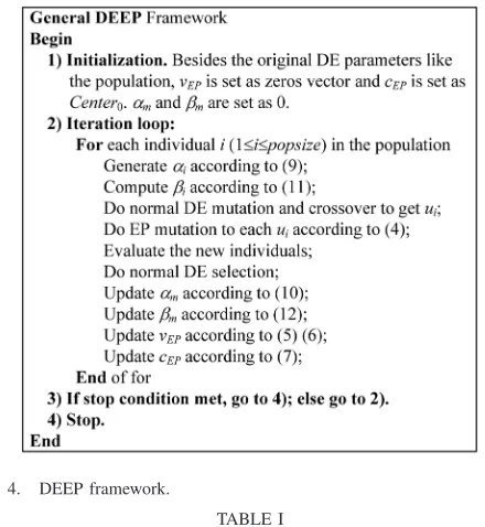
[image:5.612.324.544.51.290.2]The self-adaptation of the control parameters αi and βi relieves the user from setting those parameters for the EP mutation. Overall, the framework of DEEP is shown in Fig.4.
Fig. 4. DEEP framework.
TABLE I
PARAMETERSETTINGSUSED IN THETESTS
IV. TWODEEP ALGORITHMSILLUSTRATEDWITH
EXPERIMENTALSTUDIES
In this section, we illustrate the DEEP framework through two example DEEP algorithms and their experimental studies. We first apply DEEP to a canonical DE variant DE/rand/1 and to a state-of-the-art DE variant JADE [24] to develop a DE/rand/EP and a JADE with an EP (JADEEP), respec-tively. Experimental comparisons are then made with the original algorithms and other relevant EAs, including the DCMA-EA [21], CMA-ES [11], composite DE (CoDE) [30], self-adaptive DE (SaDE) [27], self-adaptive ensemble param-eters and strategies DE (SaEPSDE) [49] (a recent ver-sion of EPSDE), and self-adaptive DE with neighborhood search (SaNSDE) [26]. In the experiments, all algorithms are tested on the single-objective box-constrained continuous opti-mization problems in the CEC’13 benchmarks [50] and on two practical problems [52]. Test codes of JADE, CoDE, and CMA-ES are provided in [30]. Test codes of SaEPSDE and SaNSDE are obtained from their authors, respectively. Test code of DCMA-EA is implemented according to the pseudo code provided by the authors.
A. Development of DEEP From DE/rand/1 and JADE In the development of a DEEP algorithm from the traditional DE algorithm, DE/rand/1, all the settings in Section III are used. The bound handling method is adopted from JADE, as shown in
uij=
xij+uboundj
/2,if uij>uboundj
xij+lboundj
TABLE II
TESTRESULTS OFDE/RAND/EP VERSUSDE/RAND/1INTESTPROBLEMSWITHD=30, 50,AND100 (NUMBER OFFESISSHOWN IN PARENTHESES IFMEANERRORISZERO; BETTERMEANERRORSARESHOWN INBOLDFACE; SIGNIFICANTLYDIFFERENT
RESULTSAREHIGHLIGHTED INSHADE)
where u’ij is the jth dimension of the ith new individual gen-erated by (4), and ubound and lbound are the upper and lower bounds, respectively.
When developing a DEEP algorithm from JADE, F, and sCR in (4) remain associated with each individual, as used in the original DE. Two minor modifications are however, made in JADEEP for the DEEP framework. First, when we use the sCR scale factor to control the EP information in (4), a rela-tively large sCR can be used of when CR is large, for example
sCRi=
1, if CRi>0.2
CRi,otherwise (14)
because a large CR usually indicates that the algorithm is progressing well and the added EP information should be used more. The second modification involves the anchor, cEP, which is used as a promising point to guide the JADE
mutation. It is hence better to decrease the p-best guidance in the original JADE mutation as follows:
vi=xi+Fi·
xpbest−xi
+Fi·
xr1−xr2
(15)
where
Fi=Fi·(1−βi·sCRi). (16) The scale factor F’ is used to control how the p-best guidance information is decreased in relation to the mount added by (4), so as to balance JADEEP for various kinds of optimization problems.
A full pseudo code of JADEEP is shown in the Appendix. Details of the parameters used in these tests, as well as in the original DE/rand/1 algorithm, are given in Table I. The original settings of JADE remain unchanged. The settings of the control parameters used in the self-adaptation of the EP mutation are also shown in TableI.
We endeavor to use the same settings for all the test algo-rithms. The initial values of αm and βm are set to zero, which means no EP guidance is used at the very beginning. Empirically, αsig andβsig are set to a smaller value than the search range, for tests advise that they work fine as long as no extreme values are used. We shall conduct experiments to test how the range control parametersαmaxandβmaxinfluence
DEEP performance and self-adaptation ofαi andβi. We also conduct experiments on the anchor point learning parameter
λand the population center calculation parameter s.
B. Comparing the DEEP Algorithms With Their Original DEs
TABLE III
TESTRESULTS OFJADEEP VERSUSJADEINTESTPROBLEMSWITHD = 30, 50,AND100 (NUMBER OFFESISSHOWN INPARENTHESES IFMEAN ERRORISZERO; BETTERMEANERRORSARESHOWN INBOLDFACE; SIGNIFICANTLYDIFFERENTRESULTSAREHIGHLIGHTED INSHADE)
rank-sum test with a significance level 0.05) are highlighted in shade. In the last row of each table, the number of functions on which the DEEP algorithm performs significantly better than, similar to, and significantly worse than the original DE algorithm are presented.
For each test function, the mean absolute errors between the final best fitness and the theoretical best fitness and the stan-dard deviation over the given number of test runs are presented in the tables. The termination condition is the maximum num-ber of function evaluations (FEs), set to be 104per dimension, i.e., for a maximum total of D × (1E+4) FEs. If the algo-rithm converge to an absolute error smaller than 1E-9 (taken as zero) on the CEC13’ benchmarks, the algorithm terminates and the total number of FEs used are recorded and shown in parentheses.
Compared with DE/rand/1, the DEEP algorithm has been able to improve the performance on most of F1–F20 functions, while maintaining comparable performance on the composite functions F21–F28, as shown in Table II. The improvements become more salient when the dimensionality of the prob-lems increases. The DEEP algorithm has worked especially well for most functions when D increases to 100 (with a population size 400). One may be interested to measure how much the DEEP improves on such a simple function as F1, when performance on multimodal functions are at least not worse. It is seen that the numbers of FEs were reduced to 46% and 41% for D=30 and D=50, respectively. For D=100, the DE/rand/EP managed to find the theoretical minimum of
F1 with 56% of FEs of the original algorithm, which failed to reach a zero error and was terminated at the end of the predefined maximum FEs.
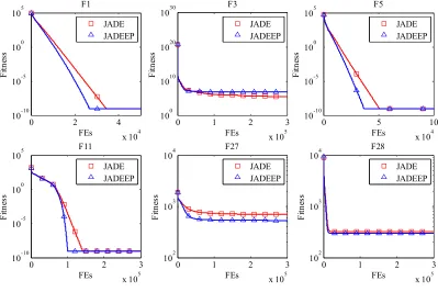
Similarly, JADEEP is also able to improve the performance over JADE, not only on unimodal functions, but also on com-posite functions, as shown in Table III. The JADEEP runs much faster than JADE on simple functions like F5, with FEs reduced to 60% when D = 100. Note that the acceleration is gained while JADEEP can perform well on complicated multimodal functions like F23 and F26. This is owing to EP providing good but not greedy guidance. For a more direct view on the improvements brought about by the DEEP framework, a search performance chart comparing JADE and JADEEP on some typical functions (D = 30) is shown in Fig.5.
We also tested the application of EP to ensemble-based DE variants with multiple strategies, such as SaDE, CoDE, and SaEPSDE, although EP showed less significant improvements. The reason might be that the greedy mutation strategy DE/best used in SaDE weakens the guidance effects of DEEP and the competing mechanism of mutation strategies in these algo-rithms weakens the effects of EP. We would hence propose in future work that dedicated EP-based mutation strategies be designed to work with the ensemble-based DE algorithms.
Fig. 5. Comparison of evolution processes between JADEEP and JADE on some representative functions.
[image:8.612.106.505.53.319.2](a) (b) (c) (d)
Fig. 6. Parameters study on (a)αmax, (b)βmax, (c)λ, and (d) s.
values of certain key parameters, the role of the two parts of EP can be more clearly understood.
The EP vector vEP is designed to help the population in
long migration, and αmax is used to control possible maxi-mum effects of vEP. The effects of vEP can be much clearer
if the initial populations happen to be far away from the global best region, especially when a promising range of the global best is unknown. We study such cases with different set-tings ofαmax and with the population initialized far from the global best. The search results on some functions are shown in Fig. 6(a) (scaled for the convenience of comparison). The results show that with a larger αmax, the search speed can be improved noticeably. This confirms that the EP vector vEP
can be helpful especially when a long migration is necessary. Thus we have recommended a largeαmaxas a suitable setting in TableI.
The EP anchor point cEP is designed to help the
popula-tion reduce wasteful detours in the search progress. In (4) the
mutation vector is affected by cEP – ui, being dragged closer
to cEP. Too much influence of cEP would cause the
popula-tion to converge prematurely, which is undesirable even when cEPis different from the current best location. Thus parameter βmax, which is used to control the effects of cEP, must be set
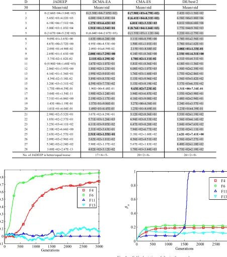
TABLE IV
JADEEP COMPAREDWITHDCMA-EA, CMA-ES,ANDDE/BEST/2 (NUMBER OFFESISSHOWN INPARENTHESES IFMEANERRORISZERO; BETTERMEANERRORSARESHOWN INBOLDFACE; SIGNIFICANTLYDIFFERENTRESULTSAREHIGHLIGHTED INSHADE)
Fig. 7. Self-adaptation ofαmin the search process.
in creating divergence when it is far from the current local best. This explains why the DEEP is able to help improve the perfor-mance on the multimodal functions, with a possibility that the cEPguidance can be quite different from the current local best.
[image:9.612.79.530.93.605.2]Another key feature of the DEEP algorithms is the popula-tion center. Parameter s is used to compute the center of the population (center of the first s best individuals) and is studied in Fig.6(d). Using either the current best individual (s=1) or the whole population (s =100 for JADE) is not as good as using our recommended value s =20. The test results show
Fig. 8. Self-adaptation ofβmin the search process.
that the population center can make a better effect of guidance than the current best in DEEP. It is also reasonable to use not all the individuals in the population to calculate the population center because some of the individuals in the population are only used to maintain divergence.
The self-adaptation mechanism is profoundly used in the literature. For other parameters in the self-adaptation, Table I
also lists their empirical values. The initial values ofαm and
[image:9.612.64.289.109.592.2]TABLE V
JADEEP COMPAREDWITHSADE, CODE, SAEPSDE,ANDSANSDE (NUMBER OFFESISSHOWN INPARENTHESES IFMEANERRORISZERO; BETTERMEANERRORSARESHOWN INBOLDFACE; SIGNIFICANTLYDIFFERENTRESULTSAREHIGHLIGHTED INSHADE)
andβm during the evolution process of JADEEP on functions F4, F6, F11, and F13. These curves show these two control parameters behave differently for different problems. Based on Fig. 7, the self-adaptation mechanism seems to be useful to find different values ofαm, large or small, negative or positive, which are proper for different functions. For example, for func-tion F6 (Rosenbrock) with a long descent corridor that would require many generations of evolution, a large αm is found to be necessary. Fig. 8 also shows that different settings of βm emerge for different functions during the evolution process.
D. Comparing JADEEP With Other Relevant Algorithms In this sub-section, the DCMA-EA [21] algorithm that directly hybridizes the DE and CMA-ES is compared in detail. More competitors include CMA-ES itself, which is a state-of-the-art CM algorithm, the DE/best/2, which can also be taken as a CM algorithm because all individuals are generated based on the current best individual, and a num-ber of state-of-the-art DE variants such as SaDE, CoDE, SaEPSDE, and SaNSDE, which use ensemble mutation strate-gies. Nonparametric Dunnett’s test [53] for multicomparisons is used here with JADEEP taken as the control algorithm against all other algorithms shown in Tables IV andV. The results that are significantly different (with a significance level 0.05) are highlighted in shade as before.
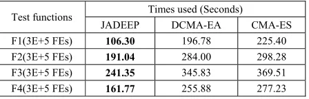
TABLE VI
COMPARISON ONTIMEOVERHEADSBETWEENJADEEP, DCMA-EA,ANDCMA-ES
[image:10.612.327.551.471.543.2]TABLE VII
[image:11.612.62.284.82.564.2]TESTRESULTS ONLENNARD-JONES ANDTERSOFFPOTENTIAL OPTIMIZATIONPROBLEMS
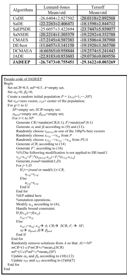
Fig. 9. Pseudo code of JADEEP.
The comparison in Table V shows that JADEEP works better than SaDE and SaNSDE on most functions. SaDE is already a fast DE algorithm and is better than the origi-nal JADE, which is especially good at unimodal functions. With the help of the EP, JADEEP improves its perfor-mance on unimodal functions while maintaining advantages on multimodal functions. JADEEP is also seen slightly bet-ter than SaEPSDE and CoDE on multimodal functions and is much faster than the two algorithms on unimodal func-tions (such as F1, F2, and F5). However, EP is less useful in JADEEP on some unimodal functions such as F3, as the original JADE algorithm itself is not good at this function.
E. Comparison of JADEEP Applied to Practical Problems Here JADEEP is applied to practical optimization problems studied in [52] which are atomic potential minimization prob-lems, important in molecular structure studies. Two potential function minimization problems were studied: the Lennard-Jones potential problem and the Tersoff potential function minimization problem. For both problems, the goal is to find the positions of a series of N atoms
X =X1,X2, . . . ,XN (17)
such that the atomic potential is minimized, where Xi is a 3-D position vector. For detailed formulation of these two problems, refer to [52].
In the experiments, JADEEP and other relevant algorithms were compared for N =10 (i.e., 10 atoms with 30 decision variables). As the population size of JADEEP could be reduced to as low as 30, this size was used in the experiments, while all settings for the other relevant algorithms remained unchanged. The results are shown in TableVII. It can be seen that JADEEP performed well and resulted in the lowest potential in these two practical problems.
V. CONCLUSION
In this paper, the reproduction mechanism of the DE has been enhanced through an evolution path, taking the advan-tages of both a CM of CMA-ES and a DM of DE. Without loss of generality, a Gaussian distribution is used in the CM as a generator for a new population centered at the mean with its path cumulatively learned during the evolutionary process. This adds a momentum in the evolution to speed up search along the trend. In the meanwhile, the DM inherent in DE uses individuals more sparsely distributed in the population without following a parametric model and hence exploration in the evolution is much retained.
Instead of directly combing the DE and the CMA-ES algo-rithms mechanistically together to develop a new algorithm, only the key CM feature of the CMA-ES, i.e., the evolution path, is used to develop DEEP efficiently for performance improvements. In particular, the direction vector of EP is uti-lized for additional mutation information and the cumulative learning weighted mean of recent EP centers is used to guide the new individuals generated by the DE. Further, CM features are self-adaptive, which helps new individuals improve quality in a new environment and simplifies algorithm design. Using the DEEP framework, we have developed and illustrated two DEEP algorithms. They have exhibited mostly better perfor-mance than the original DE and other relevant state-of-the-art algorithms.
APPENDIX
Detailed pseudo code of JADE with EP modifica-tions (JADEEP) is shown in Fig. 9. More information please contact with the corresponding author Z. H. Zhan ([email protected]).
REFERENCES
[1] J. Zhang, H. Chung, and W. L. Lo, “Clustering-based adaptive crossover and mutation probabilities for genetic algorithms,” IEEE Trans. Evol.
Comput., vol. 11, no. 3, pp. 326–335, Jun. 2007.
[2] R. Storn and K. V. Price, “Differential evolution—A simple and effi-cient heuristic for global optimization over continuous spaces,” J. Global
Optim., vol. 11, no. 4, pp. 341–359, 1997.
[3] Z. H. Zhan, J. Zhang, Y. Li, and Y. H. Shi, “Orthogonal learning par-ticle swarm optimization,” IEEE Trans. Evol. Comput., vol. 15, no. 6, pp. 832–847, Dec. 2011.
[4] B. Xue, M. J. Zhang, and W. N. Browne, “Particle swarm optimization for feature selection in classification: A multi-objective approach,” IEEE
Trans. Cybern., vol. 43, no. 6, pp. 1656–1671, Dec. 2013.
[5] Z. H. Zhan, J. Zhang, Y. Li, and H. S. H. Chung, “Adaptive parti-cle swarm optimization,” IEEE Trans. Syst., Man, Cybern. B, Cybern., vol. 39, no. 6, pp. 1362–1381, Dec. 2009.
[6] W. Chen et al., “Particle swarm optimization with an aging leader and challengers,” IEEE Trans. Evol. Comput., vol. 17, no. 2, pp. 241–258, Apr. 2013.
[7] Y. H. Li, Z. H. Zhan, S. Lin, R. Wang, and X. N. Luo, “Competitive and cooperative particle swarm optimization with infor-mation sharing mechanism for global optimization problems,” Inf. Sci., DOI: 10.1016/j.ins.2014.09.030, 2014
[8] Z. H. Zhan et al., “Multiple populations for multiple objectives: A coevo-lutionary technique for solving multiobjective optimization problems,”
IEEE Trans. Cybern., vol. 43, no. 2, pp. 445–463, Apr. 2013.
[9] M. Shen et al., “Bi-velocity discrete particle swarm optimization and its application to multicast routing problem in communication networks,”
IEEE Trans. Ind. Electron., vol. 61, no. 12, pp. 7141–7151, Dec. 2014.
[10] P. Larranaga and J. A. Lozano, Estimation of Distribution Algorithms:
A New Tool for Evolutionary Computation. Boston, MA, USA: Kluwer
Academic, 2001.
[11] N. Hansen and A. Ostermeier, “Completely derandomized self-adaptation in evolution strategies,” Evol. Comput., vol. 9, no. 2, pp. 159–195, 2001.
[12] K. Socha and M. Dorigo, “Ant colony optimization for continuous domains,” Eur. J. Oper. Res., vol. 185, no. 3, pp. 1155–1173, 2008. [13] Z. H. Zhan et al., “An efficient ant colony system based on receding
horizon control for the aircraft arrival sequencing and scheduling prob-lem,” IEEE Trans. Intell. Transp. Syst., vol. 11, no. 2, pp. 399–412, Jun. 2010.
[14] S. Tsutsui, “cAS: Ant colony optimization with cunning ants,” in Parallel
Problem Solving from Nature—PPSN IX (Lecture Notes in Computer
Science), vol. 4193. Berlin, Germany: Springer, 2006, pp. 162–171. [15] C. W. Ahn, J. An, and J.-C. Yoo, “Estimation of particle swarm
distri-bution algorithms: Combining the benefits of PSO and EDAs,” Inf. Sci., vol. 192, pp. 109–119, Jun. 2012.
[16] K. Opara and J. Arabas, “Differential mutation based on population covariance matrix,” in Parallel Problem Solving from Nature, PPSN XI (Lecture Notes in Computer Science), vol. 6238. Berlin, Germany: Springer, 2010, pp. 114–123.
[17] J. Sun, Q. Zhang, and E. P. K. Tsang, “DE/EDA: A new evolution-ary algorithm for global optimization,” Inf. Sci., vol. 169, nos. 3–4, pp. 249–262, 2005.
[18] S. Tsutsui, “Probabilistic model-building genetic algorithms in permuta-tion representapermuta-tion domain using edge histogram,” in Parallel Problem
Solving from Nature—PPSN VII. Berlin, Germany: Springer, 2002,
pp. 224–233.
[19] A. Zhou, Q. Zhang, Y. Jin, and B. Sendhoff, “Combination of EDA and DE for continuous biobjective optimization,” in Proc. IEEE Congr. Evol.
Comput., Hong Kong, 2008, pp. 1447–1454.
[20] R. V. Rao, V. J. Savsani, and D. P. Vakharia, “Teaching–learning-based optimisation: A novel method for constrained mechanical design opti-misation problems,” Comput.-Aided Design, vol. 43, no. 3, pp. 303–315, 2011.
[21] S. Ghosh, S. Das, S. Roy, S. K. Islama, and P. N. Suganthan, “A dif-ferential covariance matrix adaptation evolutionary algorithm for real parameter optimization,” Inf. Sci., vol. 182, no. 1, pp. 199–219, 2012.
[22] K. Deb, A. Anand, and D. Joshi, “A computationally efficient evolution-ary algorithm for real-parameter optimization,” Evol. Comput., vol. 10, no. 4, pp. 345–369, 2002.
[23] H. Someya, “Striking a mean- and parent-centric balance in real-valued crossover operators,” IEEE Trans. Evol. Comput., vol. 17, no. 6, pp. 737–754, Dec. 2013.
[24] J. Q. Zhang and A. C. Sanderson, “JADE: Adaptive differential evolution with optional external archive,” IEEE Trans. Evol. Comput., vol. 13, no. 5, pp. 945–958, Jun. 2009.
[25] S. Das and P. N. Suganthan, “Differential evolution: A survey of the state-of-the-art,” IEEE Trans. Evol. Comput., vol. 15, no. 1, pp. 4–31, Feb. 2011.
[26] Z. Yang, K. Tang, and X. Yao, “Self-adaptive differential evolution with neighborhood search,” in Proc. IEEE Congr. Evol. Comput., Hong Kong, 2008, pp. 1110–1116.
[27] A. K. Qin, V. L. Huang, and P. N. Suganthan, “Differential evolution algorithm with strategy adaptation for global numerical optimization,”
IEEE Trans. Evol. Comput., vol. 13, no. 2, pp. 398–417, Apr. 2009.
[28] J. Brest, S. Greiner, B. Boskovic, M. Mernik, and V. Zümer, “Self-adapting control parameters in differential evolution: A comparative study on numerical benchmark problems,” IEEE Trans. Evol. Comput., vol. 10, no. 6, pp. 646–657, Dec. 2006.
[29] W. J. Yu et al., “Differential evolution with two-level parameter adap-tation,” IEEE Trans. Cybern., vol. 44, no. 7, pp. 1080–1099, Jul. 2014. [30] Y. Wang, Z. X. Cai, and Q.-F. Zhang, “Differential evolution with com-posite trial vector generation strategies and control parameters,” IEEE
Trans. Evol. Comput., vol. 15, no. 1, pp. 55–66, Feb. 2011.
[31] W. Y. Gong, Z. H. Cai, C. X. Ling, and H. Li, “Enhanced differen-tial evolution with adaptive strategies for numerical optimization,” IEEE
Trans. Syst., Man, Cybern. B, Cybern., vol. 41, no. 2, pp. 397–413,
Apr. 2011.
[32] S. M. Elsayed, R. A. Sarker, and D. L. Essam, “An improved self-adaptive differential evolution algorithm for optimization problems,”
IEEE Trans. Ind. Informat., vol. 9, no. 1, pp. 89–99, Feb. 2013.
[33] R. Mallipeddi and P. N. Suganthan, “Differential evolution algorithm with ensemble of parameters and mutation and crossover strategies,” in Swarm, Evolutionary, and Memetic Computing. Berlin, Germany: Springer, 2010, pp. 71–78.
[34] H. Wang, S. Rahnamayan, H. Sun, and M. G. H. Omran, “Gaussian bare-bones differential evolution,” IEEE Trans. Cybern., vol. 43, no. 2, pp. 634–647, Apr. 2013.
[35] S. Das, A. Abraham, and A. Konar, “Differential evolution using a neighborhood-based mutation operator,” IEEE Trans. Evol. Comput., vol. 13, no. 3, pp. 526–552, Jun. 2009.
[36] S. M. Islam, S. Das, S. Ghosh, S. Roy, and P. N. Suganthan, “An adap-tive differential evolution algorithm with novel mutation and crossover strategies for global numerical optimization,” IEEE Trans. Syst., Man,
Cybern. B, Cybern., vol. 42, no. 2, pp. 482–500, Apr. 2012.
[37] W. Gong and Z. Cai, “Differential evolution with ranking-based muta-tion operators,” IEEE Trans. Cybern., vol. 43, no. 6, pp. 2066–2081, Dec. 2013.
[38] M. G. Epitropakis, D. K. Tasoulis, N. G. Pavlidis, V. P. Plagianakos, and M. N. Vrahatis, “Enhancing differential evolution utilizing proximity-based mutation operators,” IEEE Trans. Evol. Comput., vol. 15, no. 1, pp. 99–119, Feb. 2011.
[39] B. Y. Qu, P. N. Suganthan, and J. J. Liang, “Differential evolution with neighborhood mutation for multimodal optimization,” IEEE Trans. Evol.
Comput., vol. 16, no. 5, pp. 601–614, Oct. 2012.
[40] S. Das, A. Konar, U. K. Chakraborty, and A. Abraham, “Differential evolution with a neighborhood based mutation operator: A compara-tive study,” IEEE Trans. Evol. Comput., vol. 13, no. 3, pp. 526–553, Jun. 2009.
[41] Y. Cai and J. Wang, “Differential evolution with neighborhood and direction information for numerical optimization,” IEEE Trans. Cybern., vol. 43, no. 6, pp. 2202–2215, Dec. 2013.
[42] S. Ghosh, S. Das, A. V. Vasilakos, and K. Suresh, “On convergence of differential evolution over a class of continuous functions with unique global optimum,” IEEE Trans. Syst., Man, Cybern. B, Cybern., vol. 42, no. 1, pp. 107–124, Feb. 2012.
[43] Y. Wang and Z. Cai, “Combining multiobjective optimization with dif-ferential evolution to solve constrained optimization problems,” IEEE
Trans. Evol. Comput., vol. 16, no. 1, pp. 117–134, Feb. 2012.
[44] C. Li and S. Yang, “A general framework of multipopulation methods with clustering in undetectable dynamic environments,” IEEE Trans.
[45] S. Das, A. Mandal, and R. Mukherjee, “An adaptive differential evolu-tion algorithm for global optimizaevolu-tion in dynamic environments,” IEEE
Trans. Cybern., vol. 44, no. 6, pp. 966–978, Jun. 2014.
[46] F. Peng, K. Tang, G. Chen, and X. Yao, “Multi-start JADE with knowl-edge transfer for numerical optimization,” in Proc. IEEE Congr. Evol.
Comput., Trondheim, Norway, 2009, pp. 1889–1895.
[47] J. Sun, J. M. Garibaldi, N. Krasnogor, and Q. Zhang, “An intelligent multi-restart memetic algorithm for box constrained global optimiza-tion,” Evol. Comput., vol. 21, no. 1, pp. 107–147, 2013.
[48] A. Basak, S. Das, and K. C. Tan, “Multimodal optimization using a bi-objective differential evolution algorithm enhanced with mean dis-tance based selection,” IEEE Trans. Evol. Comput., vol. 17, no. 5, pp. 666–685, Sep. 2013.
[49] J. Derrac, S. Garcia, S. Hui, F. Herrera, and P. N. Suganthan, “Statistical analysis of convergence performance throughout the evolutionary search: A case study with SaDE-MMTS and Sa-EPSDE-MMTS,” in Proc. IEEE
Symp. Different. Evol., Singapore, 2013, pp. 151–156.
[50] J. J. Liang, B. Y. Qu, P. N. Suganthan, and A. G. Hernández-Díaz. (2014, Jan. 1). “Problem definitions and evaluation criteria for the CEC 2013 special session and competition on real-parameter optimization,” Comput. Intell. Lab., Zhengzhou Univ., Zhengzhou China, Tech. Rep. 201212 [Online]. Available:http://www.ntu.edu.sg/ home/EPNSugan/index_files/CEC2013/CEC2013.htm
[51] S. Das, A. Abraham, and A. Konar, “Differential evolution using a neighborhood-based mutation operator,” IEEE Trans. Evol. Comput., vol. 13, no. 3, pp. 526–552, Jun. 2009.
[52] S. Das and P. N. Suganthan, “Problem definitions and evaluation cri-teria for CEC 2011 competition on testing evolutionary algorithms on real world optimization problems,” Dept. Electron. Telecommun. Engg., Jadavpur Univ., Kolkata, India, and School Electr. Electron. Eng., Nanyang Technol. Univ., Singapore, Tech. Rep., 2010.
[53] C. W. Dunnett, “New tables for multiple comparisons with a control,”
Biometrics, vol. 20, no. 1, pp. 482–491, 1964.
[54] J. Zhang et al., “Evolutionary computation meets machine learning: A survey,” IEEE Comput. Intell. Mag., vol. 6, no. 4, pp. 68–75, Nov. 2011.
Yuan-Long Li (S’11) received the B.S. degree
in mathematics from Sun Yat-sen University, Guangzhou, China, in 2009, where he is currently pursuing the Ph.D. degree.
His current research interests include global opti-mization, evolutionary algorithm, time series analy-sis, deep neural network, and their applications in wireless sensor network and data center modeling.
Zhi-Hui Zhan (S’09–M’13) received the bachelor’s
and Ph.D. degrees from the Department of Computer Science, Sun Yat-sen University, Guangzhou, China, in 2007 and 2013, respectively.
He is currently a Lecturer with Sun Yat-sen University. His current research interests include par-ticle swarm optimization, differential evolution, ant colony optimization, genetic algorithms, and their applications in real-world problems.
Dr. Zhan was the recipient of the China Computer Federation Outstanding Dissertation in 2013.
Yue-Jiao Gong (S’10) received the B.S. degree
in computer science from Sun Yat-sen University, Guangzhou, China, in 2010, where she is currently pursuing the Ph.D. degree.
Her current research interests include artifi-cial intelligence, evolutionary computation, swarm intelligence, and their applications in design and optimization of intelligent transportation systems, wireless sensor networks, and RFID systems.
Wei-Neng Chen (S’07–M’12) received the
bach-elor’s and Ph.D. degrees from the Department of Computer Science, Sun Yat-sen University, Guangzhou, China, in 2006 and 2012, respectively.
He is currently an Associate Professor with the School of Advanced Computing, Sun Yat-sen University. His current research interests include swarm intelligence algorithms and their applications on cloud computing, financial optimization, oper-ations research, and software engineering. He has published over 30 papers in international journals and conferences.
Prof. Chen was the recipient of the China Computer Federation Outstanding Dissertation in 2012.
Jun Zhang (M’02–SM’08) received the Ph.D.
degree from the City University of Hong Kong, Hong Kong, in 2002.
He is currently a Changjiang Chair Professor with the School of Advanced Computing, Sun Yat-sen University, Guangzhou, China. His current research interests include computational intelligence, cloud computing, high performance computing, data min-ing, wireless sensor networks, operations research, and power electronic circuits. He has published over 100 technical papers in the above areas.
Dr. Zhang was the recipient of the China National Funds for Distinguished Young Scientists from the National Natural Science Foundation of China in 2011 and the First-Grade Award in Natural Science Research from the Ministry of Education, China, in 2009. He is currently an Associate Editor of the IEEE TRANSACTIONS ON EVOLUTIONARYCOMPUTATION, the IEEE TRANSACTIONS ONINDUSTRIALELECTRONICS, and the IEEE TRANSACTIONS ONCYBERNETICS.
Yun Li (S’87–M’90) received the B.Sc. degree
in electronics science from Sichuan University, Chengdu, China, the M.Sc. degree in electronic engineering from the University of Electronic Science and Technology of China (UESTC), Chengdu, and the Ph.D. degree in comput-ing and control engineercomput-ing from the University of Strathclyde, Glasgow, U.K., in 1984, 1987, and 1990, respectively.
From 1989 to 1990, he was with U.K. National Engineering Laboratory and Industrial Systems and Control Ltd., Glasgow, U.K. He joined the University of Glasgow, Glasgow, as a Lecturer in 1991, where he is currently a Professor of Systems Engineering. He served as a Founding Director of the University of Glasgow Singapore, Singapore, from 2011 to 2013 and acted as a Founding Director of the uni-versity’s international joint program with UESTC, Chengdu, in 2013. He established the IEEE Computer-Aided Control System Design Evolutionary Computation Working Group and the European Network of Excellence in Evolutionary Computing Workgroup on Systems, Control, and Drives in 1998. He was invited to Kumamoto University, Kumamoto, Japan, as a Visiting Professor in 2002 and is currently a Visiting Professor to UESTC and Sun Yat-sen University, Guangzhou, China. He has authored the interactive online courseware EA Demo for Evolutionary Computation and has over 180 publications.