Effect of Dynamic Stall on the Aerodynamics
of Vertical-Axis Wind Turbines
Frank Scheurich
∗University of Glasgow, Glasgow, Scotland G12 8QQ, United Kingdom
and
Richard E. Brown
†University of Strathclyde, Glasgow, Scotland G1 1XJ, United Kingdom
DOI: 10.2514/1.J051060
Accurate simulations of the aerodynamic performance of vertical-axis wind turbines pose a significant challenge for computationalfluid dynamics methods. The aerodynamic interaction between the blades of the rotor and the wake that is produced by the blades requires a high-fidelity representation of the convection of vorticity within the wake. In addition, the cyclic motion of the blades induces large variations in the angle of attack on the blades that can manifest as dynamic stall. The present paper describes the application of a numerical model that is based on the vorticity transport formulation of the Navier–Stokes equations, to the prediction of the aerodynamics of a vertical-axis wind turbine that consists of three curved rotor blades that are twisted helically around the rotational vertical-axis of the rotor. The predicted variation of the power coefficient with tip speed ratio compares very favorably with experimental measurements. It is demonstrated that helical blade twist reduces the oscillation of the power coefficient that is an inherent feature of turbines with nontwisted blade configurations.
Nomenclature
A = swept areaAst = area of the support struts,Rstcst
b = blade span
Cd0;st = zero drag coefficient of the support strut
Cn = sectional normal force coefficient,Fn=12cV12
Cn = derivative of normal force coefficient with respect to
angle of attack
Ct = sectional tangential force coefficient,Ft=12cV12
CP = power coefficient,P=12AV13
CPst;total = total power loss due to the support struts
CC
n = circulatory component of the normal force coefficient
c = chord length of the rotor blade,cb cst = chord length of the support strut,cr
Fn = sectional force acting normal to the blade chord
Ft = sectional force acting tangential to the blade chord
k = reduced frequency,c=2V1
P = power
R = reference radius of the rotor
Rst = maximum radius of the support strut,Rstz
r = sectional radius,rz S = vorticity source u = flow velocity
ub = flow velocity relative to the blade
V1 = wind speed
X,Y = deficiency functions
z = coordinate (zaxis is aligned with the rotational axis of the rotor)
= angle of attack e = effective angle of attack
= reference tip speed ratio,R=V1
= kinematic viscosity = air density
= azimuth
= angular velocity of the rotor ! = vorticity
!b = bound vorticity
I.
Introduction
T
HE number of wind turbines that have been deployed all over the world has increased considerably in recent years. The development and deployment of devices that generate useful energy from the kinetic energy contained in the wind are motivated largely by two objectives. First, there is a perceived need to reduce emissions of carbon dioxide and other pollutants by replacing fossil-fuel-fired power plants with renewable energy technologies. Second, there is a perceived demand to establish an alternative to fossil fuels in the light of thefinite nature and unequal global distribution of the known coal, oil, and gas resources.Most of the wind turbines that are currently deployed around the globe feature a horizontal-axis configuration. In recent years, there has been a resurgence of interest in vertical-axis wind turbines, however. Vertical-axis wind turbines offer several advantages over turbines with a horizontal-axis configuration. The gearbox and the generator of a vertical-axis turbine can be situated on the ground, thereby reducing the loads on the tower and facilitating the mainte-nance of the system. In addition, vertical-axis turbines are, by design, insensitive to the wind direction and therefore do not require a yaw control system. The principal advantage of these features is to enable a design that alleviates the material stress on the tower and requires fewer mechanical components. The accurate aerodynamic modeling of vertical-axis wind turbines poses a significant challenge, however. The cyclic motion of the turbine induces large variations in the angle of attack on the blades during each revolution of the rotor that result in significant unsteadiness in their aerodynamic loading. In addition, an aerodynamic interaction occurs between the blades of the turbine and the wake that is generated by the rotor. These aerodynamic char-acteristics of vertical-axis wind turbines are somewhat more complex than those of horizontal-axis configurations and are partially responsible for the fact that industrial and academic research has focused primarily on horizontal-axis turbines in the past decades, with the result that vertical-axis wind turbines are devices that are still relatively poorly understood.
Received 16 November 2010; revision received 9 February 2011; accepted for publication 13 February 2011. Copyright © 2011 by Frank Scheurich and Richard E. Brown. Published by the American Institute of Aeronautics and Astronautics, Inc., with permission. Copies of this paper may be made for personal or internal use, on condition that the copier pay the $10.00 per-copy fee to the Copyright Clearance Center, Inc., 222 Rosewood Drive, Danvers, MA 01923; include the code 0001-1452/11 and $10.00 in correspondence with the CCC.
∗Ph.D. Student, School of Engineering; [email protected].
†Professor of Computational Aerodynamics, Department of Mechanical
Engineering; [email protected].
Vol. 49, No. 11, November 2011
Historically, a range of theoretical and computational aero-dynamic methods has been used to model theflow environment around vertical-axis wind turbines, including stream-tube concepts, as proposed by Strickland [1] and Paraschivoiu [2], as well as vortex and prescribed wake methods, as suggested by Strickland et al. [3] and Coton et al. [4]. In recent years, however, increased availability of high-performance computing has allowed the aerodynamics of vertical-axis wind turbines to be computed fromfirst principles using the Navier–Stokes equations. Hansen and Sørensen [5], as well as Simão Ferreira et al. [6] have used computational schemes that solve the Reynolds-averaged Navier–Stokes equations to simulate the two-dimensional aerodynamics of an airfoil while in a planar, cyclic motion designed to emulate that of the blades of a vertical-axis wind turbine. Detached-eddy simulations of a similar airfoil configuration have been performed by Horiuchi et al. [7]. Although these con-ventional computational fluid dynamics (CFD) methods have yielded, to some extent, reasonable predictions of the behavior of simple airfoil and rotor geometries, there have been no publications in the literature, to the authors’knowledge, in which the full three-dimensional flowfield of a complex rotor system with curved, helically twisted blades has accurately been modeled from first principles.
In most CFD methods, the Navier–Stokes equations are cast into the primitive variable form, in which velocity is coupled with pressure and density, and then advanced through time numerically. This approach is known to suffer from the numerical dissipation of the vorticity in the wake that is produced by the blades of the rotor. Numerical dissipation in these computations can be reduced by refining the computational grid or, arguably, by using higher-order discretization of the governing equations. The very large number of cells that is necessary to reliably model the wake that is produced by vertical-axis wind turbines usually results in very high computational costs, however, since the accurate prediction of the blade aero-dynamic loading requires the wake to be captured, and thus vorticity to be conserved, for many rotor revolutions. An alternative method that can overcome the problem of excessive numerical dissipation that is associated with the primitive variable formulation of the Navier–Stokes equations is to conserve vorticity explicitly after casting the Navier–Stokes equations in vorticity–velocity form. This approach represents the basis of the vorticity transport model (VTM), which was developed by Brown [8] and extended by Brown and Line [9] and has been used for the simulations that are documented in the present paper. The VTM is described in more detail in Sec. II.
In the present study, the VTM has been used to analyze the aerodynamic performance of a commercial vertical-axis wind tur-bine that comprises blades that are helically twisted around the rotational axis of the turbine. The VTM-predicted variation of the power coefficient with tip speed ratio agrees very satisfactorily with the experimental measurements of the same turbine that were per-formed by Penna [10]. The helical twist of the turbine is shown to reduce the amplitude of the oscillations of the power coefficient at the blade-passage frequency that are an inherent feature of turbines with nontwisted blade configurations.
II.
Computational Aerodynamics
The aerodynamic performance of a vertical-axis wind turbine has been simulated using the VTM. The VTM was originally developed for simulating the flowfield surrounding helicopters, but is an aerodynamic tool that is also applicable to the study of wind turbine rotors. Indeed, Scheurich et al. [11] have compared VTM predictions against experimental measurements of the blade aerodynamic loading of a straight-bladed vertical-axis wind turbine that were made by Strickland et al. [12]. Furthermore, Scheurich and Brown [13] and Scheurich et al. [14] have used the VTM to investigate the effect of obliqueflow conditions and rotor geometry, respectively, on the aerodynamic performance of vertical-axis wind turbines.
The VTM enables the simulation of wind turbine aerodynamics and performance by providing a high-fidelity representation of the dynamics of the wake that is generated by the rotor. The VTM consists of an outer model in which the dynamics of the wake that is
generated by the rotor are calculated based on basicfluid dynamics principles and an inner, lifting-line-type, blade aerodynamic model in which the aerodynamic loads on the blades of the rotor are determined. The approach is outlined below but the reader is referred to [8,9] for more detailed information.
A. Wake Model
In contrast to more conventional computationalfluid dynamics techniques in which theflow variables are pressure, velocity, and density, the VTM is based on the vorticity–velocity form:
@
@t!u r!! ruSr
2! (1)
of the unsteady incompressible Navier–Stokes equation. The advection, stretching, and diffusion terms within Eq. (1) describe the changes in the vorticityfield!, with time at any point in space, as a function of the velocityfielduand the kinematic viscosity. The physical condition that vorticity may neither be created nor destroyed within theflow, and thus may only be created at the solid surfaces that are immersed within thefluid, is accounted for using the vorticity source termS. The vorticity source term is determined as the sum of the temporal and spatial variations in the bound vorticity!bon the
turbine blades, and so
S d
dt!bubr !b (2)
whereubis the local velocity at the blade section that comprises
contributions from the circumferential velocity of the blade, the freestream velocity and the velocity component that is induced by the wake. Thefirst term in Eq. (2) represents the shed vorticity and the second term represents the trailed vorticity from the blade. In the VTM, Eq. (1) is discretized infinite volume form using a structured Cartesian mesh within a domain that encloses the turbine rotor; it is then advanced through time using an operator-splitting technique. For calculations of full-scale turbine aerodynamics, the assumption is usually made that the Reynolds number within the computational domain is sufficiently high so that the equations governing theflow in the wake of the rotor may be solved in inviscid form and, thus, that the viscosityin Eq. (1) can be set equal to zero. The numerical diffusion of vorticity within theflowfield surrounding the wind turbine is kept at a very low level by using a Riemann solver based on the weighted averageflux method developed by Toro [15] to advance the vorticity convection term in Eq. (1) through time. This approach permits many rotor revolutions to be captured without significant spatial smearing of the wake structure and at a very low computational cost, compared with those techniques that are based on the pressure–velocity– density formulation of the Navier–Stokes equations. Dissipation of the wake does still occur, however, through the proper physical process of natural vortical instability. Most important in the present context, the shed-vorticity distribution behind the blade is fully resolved using this approach. The influence of the shed vorticity on the unsteady aerodynamic response of the system is thus captured directly in the simulations without the need for empirical modeling of the response of the blade. The implications of this inherent feature of the VTM on the coupling between the wake and blade models is discussed in the following section.
B. Blade Aerodynamic Model
Various methods can be used to determine the bound vorticity on the blades, and thus to calculate the source termSin Eq. (2), thereby coupling the outer wake model with the inner model for the blade aerodynamic loading. A modified version of the Weissinger-L lifting-line model [16] was used within the version of the VTM that was employed in this study in order to model the bound vorticity distribution on the blades of the rotor. The geometric angle of attack of the blades of a vertical-axis wind turbine can easily exceed20,
aerodynamics of vertical-axis wind turbines are to be predicted accurately. The Weissinger-L method has thus been modified in the VTM by using two-dimensional experimental airfoil data in order to represent the real performance of any given airfoil. The modification is carried out by scaling the strength of bound circulation by the
“real“lift coefficient at the specific angle of attack. The“real“lift coefficient is provided either by look-up tables that contain the experimentally measured quasi-static two-dimensional character-istics of the rotor blade sections or by a dynamic stall model. In this paper it is shown, however, that the inclusion of an accurate repre-sentation of dynamic stall is crucial if the aerodynamics of vertical-axis wind turbines are to be predicted reliably.
The effect of dynamic stall on the aerodynamic performance of an airfoil was accounted for in the present study by using a semi-empirical model that follows the approach suggested by Leishman and Beddoes [17] but has been modified to couple the model to the VTM, as explained below. The Leishman–Beddoes model was originally developed to simulate the effect of dynamic stall on the blades of a helicopter rotor. Gupta and Leishman [18] demonstrated, however, that a modified version of the original Leishman–Beddoes model can be used to represent the dynamic stall of airfoils that are comparable to those used for horizontal-axis wind turbines.
The approach that was proposed by Leishman and Beddoes [17] to model separatedflow follows directly from the Kirchhoff–Helmholtz theory that is described by Thwaites [19], among others. Hereby, the trailing-edge separation phenomenon in the stall and poststall regions of a lifting body is considered as a specific case of the Kirchhoffflow so that the sectional normal force coefficientCnand
the sectional tangential force coefficientCtcan be approximated as a
function of the position at which theflow separates from the upper
surface of the airfoil. The Leishman–Beddoes model consists of three subroutines. Thefirst and second account for the unsteady airloads in attached flow and in separatedflow, and the third represents the airloads that are induced if a dynamic stall vortex forms near the leading edge and convects over the chord of the airfoil. The airfoil performance under unsteady (but attached)flow conditions is calcu-lated by a superposition of indicial aerodynamic response functions derived from afinite difference approximation to Duhamel’s integral. The indicial response, or in other words, the response to a step change in forcing, can be expressed as the steady state response added to which is a deficiency function that decays exponentially with time. Consequently, the normal force due to circulation that arises from step changes in angle of attack,CC
ni, is expressed by
CC
niCniXiYi Cnei (3)
whereCn is the derivative of the normal force coefficient with
respect to the angle of attack,iis the index of the current time sample, andXandYare deficiency functions that have time constants that are derived from experimental measurements.
The induced velocity due to vortex shedding in unsteady attached
flow is already accounted for in the VTM, however, by thefirst term in Eq. (2). In other words, the angle of attack in unsteady attached
flow that is calculated within the VTM for each time step is identical to the equivalent angle of attackeiin Eq. (3). Thus, the effects of the
deficiency functionsXandYin Eq. (3) are implicitly included in the VTM by Eq. (2).
Angell et al. [20] investigated the occurrence of dynamic stall on an airfoil that was cycled in such a way as to mimic the changes in angle of attack that the airfoil would experience on a vertical-axis
−15 −10 −5 0 5 10 15
−1.5 −1.0 −0.5 0.0 0.5 1.0 1.5
Geometric angle of attack, α [deg]
Sectional nor
mal f
o
rce coefficient, C
n VTM + static airfoil data
Experiment
a) Normal force, static airfoil data
−15 −10 −5 0 5 10 15
−1.5 −1.0 −0.5 0.0 0.5 1.0 1.5
Geometric angle of attack, α [deg]
Sectional nor
m
al f
o
rce coefficient, C
n VTM + dynamic stall model
Experiment
b) Normal force, dynamic stall model
−15 −10 −5 0 5 10 15
−0.02 0.00 0.02 0.04 0.06 0.08 0.10 0.12 0.14 0.16 0.18 0.20
Geometric angle of attack, α [deg]
Sectional tangential f
orce coefficient, C
t
VTM + static airfoil data
Experiment
c) Tangential force, static airfoil data
−15 −10 −5 0 5 10 15
−0.02 0.00 0.02 0.04 0.06 0.08 0.10 0.12 0.14 0.16 0.18 0.20
Geometric angle of attack, α [deg]
Sectional tangential f
o
rce coefficient, C
t
VTM + dynamic stall model
Experiment
d) Tangential force, dynamic stall model
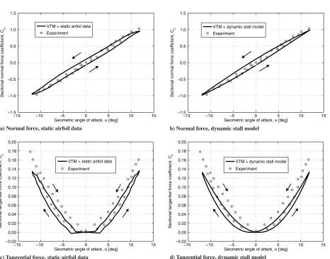
Fig. 1 VTM-predicted normal and tangential force coefficients on a NACA 0015 airfoil based on static airfoil data (left) and in conjunction with its dynamic stall model (right), compared with experimental measurements of dynamic stall made by Angell et al. [20] when the airfoil was operated at
Re800;000. A skewed sinusoidal variation of angle of attack (with amplitude 11.90) was used in order to represent vertical-axis wind turbine
[image:3.585.64.530.354.719.2]wind turbine. Their experiments revealed that the tangential force coefficient can become negative under deep stall conditions, as is shown in the next section of this paper. This observation conflicts with the Kirchhoff theory, since the tangential force coefficient, based on this theory, is always greater than or equal to zero irrespective of theflow state. Sheng et al. [21] thus suggested a modification to the model of the tangential force coefficient. The modification includes an additional parameter that accounts for negative tangential forces at low Mach numbers in deep stall. The Leishman–Beddoes-type dynamic stall model that is implemented in the VTM includes this modification for the calculation of the tangential force coefficient and has also further been modified as suggested by Niven and Galbraith [22], to account for vortex inception at low Mach numbers.
C. Validation
Before the VTM and its dynamic stall model are applied to model the aerodynamics of vertical-axis wind turbines, it is essential to establishfirst that the effect of dynamic stall on the blade aero-dynamic loading is correctly simulated by the approach. The variation of the VTM-predicted normal and tangential force
coef-ficients of a NACA 0015 airfoil in a dynamic stall test, compared with experimental measurements that were made by Angell et al. [20] are shown in Figs. 1–3. The airfoil was operated at a Reynolds number of 800,000, a Mach number of 0.064 and a reduced frequency of 0.05. Thegeometricangle of attackof the blade of a rotating vertical-axis wind turbine is a function only of the tip speed ratioand the azimuth angle , such that
arctan
sin
cos
(4)
The experiment was designed to emulate the time histories of the angle of attack encountered by the blades of a vertical-axis wind turbine by oscillating a fixed blade according to the skewed sinusoidal function that is given in Eq. (4). The maximum of the angle of attack was varied between test runs in order to simulate the time histories of the angle of attack at different tip speed ratios. Thus, the skewed sinusoidal variations of the geometric angle of attack on an airfoil, for which comparisons between VTM predictions and the experimental measurements [20] are presented in Figs. 1–3, yield conditions that are comparable to those experienced by the blade sections of a vertical-axis wind turbine when operating at local tip speed ratios of 4.85, 3.40, and 2.70, respectively. These tip speed ratios are equivalent to high, moderate, and low tip speed ratios within the range at which lift-driven vertical-axis wind turbines typically operate. Results of VTM simulations with its dynamic stall model and with a quasi-steady representation of airfoil behavior are presented in Figs. 1–3 in order to allow the effect of dynamic stall on the accuracy with which the behavior of the airfoil is modeled to be evaluated.
Figure 1 shows that, at a high tip speed ratio, the normal and tangential force coefficients that are predicted by the VTM when quasi-steady airfoil data is used are almost identical to the VTM prediction in conjunction with a dynamic stall model. This is a simple consequence of the variation of the angle of attack at high tip speed ratios being predominantly in the regime in which the aerodynamic behavior of the airfoil is linear.
−20 −15 −10 −5 0 5 10 15 20
−2.0 −1.5 −1.0 −0.5 0.0 0.5 1.0 1.5 2.0
Geometric angle of attack, α [deg]
Sectional nor
mal f
o
rce coefficient, C
n
VTM + static airfoil data
Experiment
a) Normal force, static airfoil data
−20 −15 −10 −5 0 5 10 15 20
−2.0 −1.5 −1.0 −0.5 0.0 0.5 1.0 1.5 2.0
Geometric angle of attack, α [deg]
Sectional nor
mal f
orce coefficient, C
n
VTM + dynamic stall model Experiment
b) Normal force, dynamic stall model
−20 −15 −10 −5 0 5 10 15 20
−0.05 0.00 0.05 0.10 0.15 0.20 0.25 0.30 0.35
Geometric angle of attack, α [deg]
Sectional tangential f
orce coefficient, C
t
VTM + static airfoil data
Experiment
c) Tangential force, static airfoil data
−20 −15 −10 −5 0 5 10 15 20
−0.05 0.00 0.05 0.10 0.15 0.20 0.25 0.30 0.35
Geometric angle of attack, α [deg]
Sectional tangential f
orce coefficient, C
t
VTM + dynamic stall model Experiment
d) Tangential force, dynamic stall model
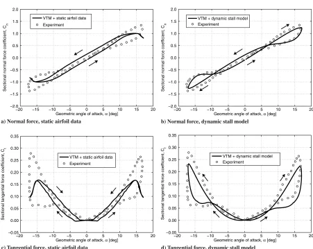
Fig. 2 VTM-predicted normal and tangential force coefficients on a NACA 0015 airfoil based on static airfoil data (left) and in conjunction with its dynamic stall model (right), compared with experimental measurements of dynamic stall made by Angell et al. [20] when the airfoil was operated at
Re800;000. A skewed sinusoidal variation of angle of attack (with amplitude 17.10) was used in order to represent vertical-axis wind turbine
[image:4.585.67.518.359.718.2]At a moderate tip speed ratio, it is clear that the use of static airfoil data is inadequate to capture the behavior of the airfoil, as is shown in Figs. 2a and 2c. The hysteresis that occurs in the experiment is not captured and the peaks in the measured aerodynamic coefficients are considerably underpredicted by the VTM simulations that are based on static airfoil data. The airfoil behavior is represented much more accurately when a dynamic stall model is used within the VTM, as demonstrated in Figs. 2b and 2d. Although the experimental mea-surements are not perfectly matched, the VTM simulations that include the dynamic stall model agree reasonably well with both measured normal and tangential force coefficients in terms of magnitudes and shapes of the hysteresis loops. According to the measurements made by Angell et al. [20], the static stall angle of the NACA 0015 airfoil is 14if the chord Reynolds number is 800,000.
Interestingly, Fig. 2 shows the normal and tangential force coefficients to be influenced significantly by unsteady aerodynamic effects, even in conditions in which the static stall angle of the NACA 0015 airfoil is only exceeded by a small amount.
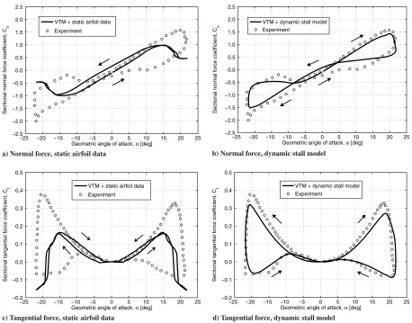
The deficiencies of the model when static airfoil data is used become even more apparent at low tip speed ratio, as shown in Figs. 3a and 3c. Figures 3b and 3d reveal, however, that the VTM predictions are improved considerably when the dynamic stall model is used in the analysis.
Although some minor discrepancies between the experimental measurements and the VTM predictions that include the dynamic stall model are apparent, the variations with angle of attack of the VTM-predicted normal and tangential force coefficients agree, overall, reasonably well with the experimental measurements, particularly in terms of the shapes and sizes of the hysteresis loops.
These comparisons thus provide confidence that the effect of dynamic stall is satisfactorily accounted for in the VTM when its dynamic stall model is used to represent the blade aerodynamics.
III.
VTM Prediction of Turbine Performance
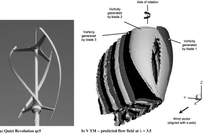
The VTM has been used to model the aerodynamics of the qr5 commercial vertical-axis wind turbine that is produced by Quiet Revolution, Ltd., a U.K.-based manufacturer. The turbine consists of three blades with NACA four-digit airfoil sections that are helically twisted around the rotational axis of the rotor, as shown in Fig. 4a. The radius of each blade section, in other words the distance between the rotational axis and each individual section, varies along the blade span. The turbine height and the reference radiusRare 5 and 1.5 m, respectively. The blades of the turbine are inclined so that the blade tip at the top of the turbine, denoted asz=b1, precedes the tip at the bottom of the turbine, denoted asz=b0, by 120in azimuth. Thedefinition is made that the reference blade is located at 0azimuth
when the blade tip at the top of the rotor, thus the blade section at z=b1, is aligned with the freestream velocity vector and its leading edge faces the wind. The turbine has support struts close to the top and the bottom that connect the blades to the shaft of the rotor. For simplicity, these support struts were not modeled within the numerical simulation. The influence of the struts on the turbine per-formance would appear to become important, however, at higher tip speed ratios, as will be discussed later in this paper. Theflowfield that is predicted by the VTM to surround the turbine is visualized by plotting an isosurface of vorticity in Fig. 4b.
−25 −20 −15 −10 −5 0 5 10 15 20 25
−2.5 −2.0 −1.5 −1.0 −0.5 0.0 0.5 1.0 1.5 2.0 2.5
Geometric angle of attack, α [deg]
Sectional nor
mal f
orce coefficient, C
n
VTM + static airfoil data
Experiment
a) Normal force, static airfoil data
−25 −20 −15 −10 −5 0 5 10 15 20 25
−2.5 −2.0 −1.5 −1.0 −0.5 0.0 0.5 1.0 1.5 2.0 2.5
Geometric angle of attack, α [deg]
Sectional nor
mal f
o
rce coefficient, C
n VTM + dynamic stall model
Experiment
b) Normal force, dynamic stall model
−25 −20 −15 −10 −5 0 5 10 15 20 25
−0.2 −0.1 0.0 0.1 0.2 0.3 0.4 0.5
Geometric angle of attack, α [deg]
Sectional tangential f
orce coefficient, C
t VTM + static airfoil data
Experiment
c) Tangential force, static airfoil data
−25 −20 −15 −10 −5 0 5 10 15 20 25
−0.2 −0.1 0.0 0.1 0.2 0.3 0.4 0.5
Geometric angle of attack, α [deg]
Sectional tangential f
o
rce coefficient, C
t VTM + dynamic stall model
Experiment
d) Tangential force, dynamic stall model
Fig. 3 VTM-predicted normal and tangential force coefficients on a NACA 0015 airfoil based on static airfoil data (left) and in conjunction with its dynamic stall model (right), compared with experimental measurements of dynamic stall made by Angell et al. [20] when the airfoil was operated at
Re800;000. A skewed sinusoidal variation of angle of attack (with amplitude 21.80) was used in order to represent vertical-axis wind turbine
[image:5.585.64.522.363.722.2]A. Power Coefficient
Figure 5 shows the VTM-predicted variation of power coefficient, CP, with tip speed ratio,, as compared with experimental
meas-urements that were made by Penna [10] on a full-scale qr5 turbine in the 9 by 9 m wind tunnel of the Canadian National Research Council. Blockage effects in the wind tunnel were accounted for by estimating analytically the interference of the wind-tunnel walls on the mea-surements. This estimation was applied as a correction to the measurements and included in the presented data. The experiment was carried out with a constant freestream velocity of9 m=s. The average blade Reynolds number, based on the circumferential velocityR, was thus approximately 400,000 for tip speed ratios near the center of the turbine’s operating range. Figure 5a shows significant discrepancies between the experimental measurements and VTM simulations when static airfoil data is used in the simulation; indeed, the trend of the power coefficient with tip speed ratio is completely mispredicted. Interestingly, the measured power coefficients are overpredicted when the tip speed ratio is greater than or equal to four, whereas they are underpredicted at low tip speed ratios. This characteristic behavior of the predictions that are based on static airfoil data is a result of the tangential force coefficient being largely underpredicted at low tip speed ratios, as shown in Fig. 3c. The overprediction of the power coefficient at high tip speed ratios, in contrast, is a result of the hysteresis loop that is associated with dynamic stall on the blades not being captured and thus the net tangential force coefficient being overpredicted by the simulation, as indicated in Fig. 2c. It is thus not surprising that an analysis that is based on static airfoil data overpredicts the power coefficient of the qr5 at high tip speed ratios, since the distribution of the angle of attack along the blade span, as shown in Fig. 6a, suggests that the blade of the qr5 (and, in particular, its lower tip) is subject to unsteady aerodynamic effects, even when the turbine is operated at high tip speed ratios.
Very satisfactory agreement between experimental measurements and simulation is obtained, in contrast, when the VTM is employed in conjunction with its dynamic stall model, as shown in Fig. 5b. The VTM simulation results (“stars“in Fig. 5b) agree very well with the experimental measurements when the tip speed ratio is less than that for the maximum power coefficient, whereas they overpredict the measured power coefficients at higher tip speed ratios. In particular, the tip speed ratio at which the maximum power coefficient is
Fig. 4 The Quiet Revolution qr5 vertical-axis wind turbine (courtesy of Quiet Revolution, Ltd.) (left) and the VTM-predictedflowfield of the turbine visualized by plotting an isosurface of vorticity (right).
0 1 2 3 4 5 6
0.00 0.05 0.10 0.15 0.20 0.25 0.30 0.35 0.40 0.45 0.50
Tip speed ratio, λ
P
o
w
e
r coefficient, C
P
Experiment VTM + static airfoil data
a) VTM simulations based on static airfoil data
0 1 2 3 4 5 6
0.00 0.05 0.10 0.15 0.20 0.25 0.30 0.35 0.40 0.45 0.50
Tip speed ratio, λ
P
o
w
er coefficient, C
P
Experiment
VTM + dynamic stall model
VTM + dynamic stall model + drag of struts
[image:6.585.312.535.357.702.2]obtained and the maximum power coefficient itself are very well predicted: arguably better than has previously been possible using any other numerical technique. The reason for the disagreement between VTM simulation results and experimental measurements at higher tip speed ratios is most likely the additional drag that is due to the support struts that connect the rotor blades with the shaft of the turbine (see Fig. 4a). These struts were not modeled within the simulation.
An estimation of the drag that is caused by the struts, and thus the loss in overall power of the qr5 turbine is given below. The loss of power that is due to the parasite drag of one support strut,CPst, can be
estimated as
CPst 1 2
Z2
0 ZR
st
0
Cd0;strV1cos 2cstr drd (5)
whereis the air density,Cd0;stis the zero drag coefficient of the strut,
Rstis the maximum radius of the strut,ris the local circumferential
velocity,V1is the wind speed, is the azimuth, andcstis the local
chord of the strut.
By integrating Eq. (5) for each strut, the total loss of power due to the support structure can be expressed as a nondimensionalized power coefficient:
CPst;total
XN
i1
1 4Cd0;st
Ai
st
A
Ri
st
R
Ri
st
R
3
3
(6)
whereNis the number of the support struts,Ast is the area of the struts, andAis the swept area of the turbine. The power loss that is caused by the drag generated by the support struts is a function of the tip speed ratio cubed, as shown by the last term in Eq. (6). The power coefficients of the qr5 that are predicted by the VTM when the
estimated drag generated by the struts is included (diamonds in Fig. 5b), are in better agreement with the experimental measurements at the tip speed ratios 4.5 and 5.0, although the measured power coefficients at these tip speed ratios are still overpredicted by the numerical simulations. This indicates that there are larger, as yet unresolved power losses within the system that can not be accounted for solely by this simplistic model for the parasite drag of the struts. The simple drag estimation shows, however, that the discrepancy between VTM simulation and experimental measurements at the highest tip speed ratio, can partially be explained by the struts not being included in the numerical model.
B. Angle of Attack and Blade Aerodynamic Loading
The effect of the helical blade twist on the blade aerodynamic loading and the wake that is generated by the blades are discussed in more detail in the following section.
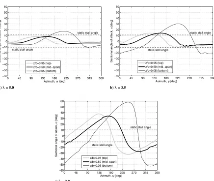
It is well known that the geometric angle of attack of the blades of a vertical-axis wind turbine varies within one rotor revolution, as indicated by Eq. (4). The maximum angle of attack of each section of the blade occurs when the section is located upstream of the axis of rotation and close to the position at which its chord is perpendicular to the wind velocity vector. The geometry of the qr5 features a sectional radius that is maximum close to the midspan of the blade and decreases toward the tips of the blades, in other words toward the top and the bottom of the rotor. The smaller sectional radius of the portions of the blade closest to the blade tips (in particular, at the lower end of the rotor) results in a smallereffectivetip speed ratio, compared with the tip speed ratio close to the midspan of the blade. Since both the maximum geometric and aerodynamic angle of attack of the blade sectionincreasewhen the tip speed ratiodecreases, the sectional angles of attack are higher at the top and, in particular, at the
0 45 90 135 180 225 270 315 360
−60 −50 −40 −30 −20 −10 0 10 20 30 40 50 60
Azimuth,ψ [deg]
Sectional angle of attac
k,
α
[deg]
z/b=0.95 (top) z/b=0.50 (mid−span) z/b=0.05 (bottom)
static stall angle
static stall angle
0 45 90 135 180 225 270 315 360
−60 −50 −40 −30 −20 −10 0 10 20 30 40 50 60
Azimuth,ψ [deg]
Sectional angle of attac
k
,
α
[deg]
z/b=0.95 (top) z/b=0.50 (mid−span) z/b=0.05 (bottom)
static stall angle
static stall angle
0 45 90 135 180 225 270 315 360
−60 −50 −40 −30 −20 −10 0 10 20 30 40 50 60
Azimuth,ψ [deg]
Sectional angle of attac
k,
α
[deg]
z/b=0.95 (top) z/b=0.50 (mid−span) z/b=0.05 (bottom)
static stall angle
static stall angle
a) λ = 5.0 b) λ = 3.5
c) λ = 2.0
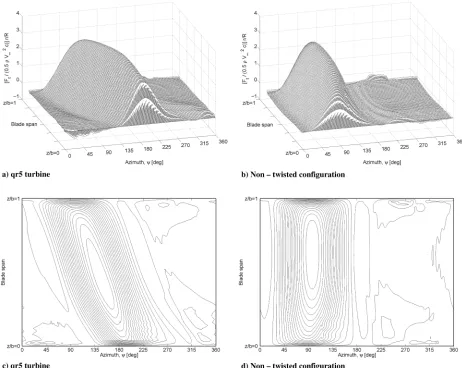
[image:7.585.76.512.375.743.2]bottom of the turbine than at the midspan of the blade, as depicted in Fig. 6. The variation of radius along the blade also results in a variation of the local velocity, however. Consequently, the tangential force, being a function of the local velocity and the local angle of attack, is somewhat more evenly distributed along the blade span, compared with the normal force, as shown in Figs. 7a, 7c, 8a, and 8c. The normal force, in contrast, is maximum on the upper portion of the blade and decreases steadily toward the lower tip of the blade. The blade aerodynamic loading of the qr5 turbine is compared in Figs. 7 and 8 to that of a second turbine that has blades with identical airfoil sections and curvature as the qr5 turbine. The blades of this second turbine are not twisted, however, in order to compare the blade aerodynamic loading produced by a nontwisted turbine to that generated by a helically twisted configuration. Figures 7b, 7d, 8b, and 8d indicate that a peak in the blade loading of the nontwisted configuration is produced close to 90azimuth. This is where the
freestream velocity vector is orthogonal to the blade chord, resulting in a high angle of attack and an associated peak in the blade loading. The prime consequence of helical twist is the distribution of the blade loading over a greater azimuth range, as shown in Figs. 7a, 7c, 8a, and 8c. The implications of these inherent differences in the char-acteristics of the two turbines on the variations with azimuth of the power coefficient that they produce will be discussed in more detail later in this paper.
Scheurich et al. [11] investigated the aerodynamic loading of the blades of a straight-bladed vertical-axis wind turbine and showed that, downstream of the axis of rotation, the blades of the turbine interact with a region of vorticity that predominantly consists of tip vortices that were trailed from the blades in previous rotor revolutions. These blade–vortex interactions resulted in impulsive changes to the angle of attack and, consequently, the blade aero-dynamic loading. Comparable observations were made by Simão
Ferreira [23] who carried out experimental and computational studies on a straight-bladed vertical-axis wind turbine. Similar observations were also made by Scheurich et al. [14] who simulated the performance of a straight-bladed and a curved-bladed vertical-axis wind turbine and compared their results to a turbine with a helically twisted blade configuration. They observed strong blade– vortex interactions for both the helically twisted and the straight-bladed configurations, whereas the blade–vortex interactions seemed to be less severe for the curved-bladed turbine. Interestingly, these blade–vortex interactions also seem to be significantly alleviated for the qr5 turbine that is investigated in the present study. This is most likely due to the greater amount of blade curvature, and thus reduced radius, close to the blade tips of the qr5, compared with that of the helically twisted turbine and the straight-bladed turbine that were investigated in the previous studies [14,23] mentioned above. Since the local radius at the blade tip is small, blade–vortex interactions occur after the tip vortex has convected over a shorter distance, compared with the situation for a less curved or a straight-bladed turbine. Consequently, the newly created tip vortices interact with the blade well before the vortices have time to convect any appreciable distance toward the horizontal centerline of the turbine. The interaction between the tip vortices and the blade of the qr5 turbine is thereby confined to the portion of the blade that is closest to the lower tip of the blade, as indicated in Fig. 7c.
The interactions between the blades and the vorticity within the wake of the qr5 turbine is visualized in Fig. 9. Thefigure shows the vorticity distribution on a plane that contains the axis of the turbine and that is aligned with the wind direction. The vorticity distribution is depicted at the instant of time when blade 1 is located at 170
azimuth. The flowfield is represented using contours of the component of vorticity perpendicular to the plane in order to emphasize the vortices that are trailed from the tips of the blades. The
[image:8.585.306.526.46.203.2]dark rendering corresponds to vorticity with a clockwise sense of rotation, and the light rendering corresponds to vorticity with a counterclockwise sense. Based on the observations made in the previous studies [14,23] mentioned above, one might expect inter-actions between the blades and the tip vortices to occur at the top of the qr5 turbine, since the radius of the blade is greater at the top than at the bottom of the turbine. Weak interactions between the tip vortices and the blades of the qr5 turbine occur at the bottom of the turbine, however, whereas these interactions seem to be absent at the top of the turbine, as shown in Fig. 7c. This phenomenon can be understood once it is realized that the distribution of vorticity within the wake is asymmetric with respect to the horizontal centerline of the turbine. The asymmetry of the vorticity within the wake, and the different strength of the tip vortices, is caused by a combination of asymmetric blade curvature with respect to the horizontal centerline and, more important, by the helical twist of the blades. The convection of the vortex that is trailed from the upper tip is, due to the corresponding skewness of the wake, less inclined toward the centerline than the one trailed from the lower tip, as indicated in Fig. 9. The vortex trailed from the upper tip does thus not interact significantly with the blades once downstream of the axis of rotation. The trajectory of the vortex that is trailed from the lower tip, in contrast, is more inclined toward the horizontal centerline of the rotor than that of the upper tip. This consequently results in interactions between the blades of the rotor and the vortices that are trailed from the lower tips as the blades pass downstream of the axis of rotation.
Interestingly, Figs. 7b and 7d show that the aerodynamic loading on the blades of the nontwisted turbine is influenced by interactions between the blade and the tip vortices at both the top and the bottom of the turbine. Since the radius of the lower portion of the blade is smaller than at the top of the turbine these blade–vortex interactions
occur at smaller azimuth angles than the interactions at the top of the turbine; this is simply because the greater radius at the top of the turbine enables the vortices trailed from the upper tips of the blades to convect a longer distance before they interact with the upper portions of the blades as they pass downstream of the axis of rotation.
A study of the distribution of the torque that is produced by each section of the rotor blades, in other words the product between the
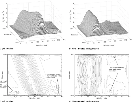
Fig. 8 VTM-predicted variation with azimuth of the nondimensional normal forces along the blade spans of the qr5 turbine (left) and the rotor with nontwisted blades (right) at3:5.
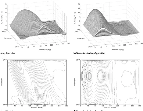
[image:9.585.57.526.45.410.2] [image:9.585.310.537.530.719.2]local tangential force and the local sectional radius, is presented in Fig. 10. The VTM-predicted variation of sectional torque is shown for the qr5 turbine and for the equivalent nontwisted turbine confi g-uration. Figures 10a and 10c show the VTM-predicted variation with azimuth of the nondimensional sectional torque along the blade span of the qr5 and reveal that the sectional torque is distributed smoothly along the blade span for a large portion of the blade.
Figure 11a shows the variation of the power coefficient with azimuth for three different tip speed ratios, whereas Fig. 11b depicts
the minimum and maximum of the power coefficient in each revolution. The variation of the power coefficient features three dominant peaks caused by the three blades of the rotor. Although the variations with azimuth of the power coefficient that is produced by the qr5 are reduced, compared with those of the nontwisted turbine configuration, as shown in Fig. 12, the amount of helical twist of the qr5 is insufficient to distribute the sectional torque evenly around the azimuth. Scheurich et al. [14] showed that the variation with azimuth of the power coefficient can be reduced even further if blade twist is
Fig. 10 VTM-predicted variation with azimuth of the nondimensional sectional torque along the blade spans of the qr5 turbine (left) and the rotor with nontwisted blades (right) at3:5.
0 45 90 135 180 225 270 315 360
0.00 0.05 0.10 0.15 0.20 0.25 0.30 0.35 0.40 0.45 0.50 0.55
Azimuth,ψ [deg]
P
o
w
er coefficient, C
P
λ = 2.0 λ = 3.5 λ = 5.0
a) Variation of power coefficient with azimuth
0 1 2 3 4 5 6
0.00 0.05 0.10 0.15 0.20 0.25 0.30 0.35 0.40 0.45 0.50 0.55
Tip speed ratio, λ
P
o
w
e
r coefficient, C
P
[image:10.585.302.523.49.203.2]b) Variation of mean power coefficient
[image:10.585.68.517.562.735.2]appropriately combined with blade curvature, in other words if helical twist and local radius are carefully chosen for each blade section. The azimuth at which the maximum power coefficient is obtained during each revolution differs between the qr5 and the nontwisted configuration. This is simply a consequence of the maxi-mum torque being shifted toward higher azimuth angles for the qr5 turbine, compared with the nontwisted configuration, as indicated in Fig. 10.
IV.
Conclusions
The vorticity transport model has been used to simulate the three-dimensionalflowfield surrounding a commercial vertical-axis wind turbine that consists of three blades that are helically twisted around the rotational axis of the rotor. The predicted variation of the power coefficient agrees very favorably with experimental measurements of the same turbine. It was demonstrated that an appropriate imple-mentation of a dynamic stall model is essential if the performance of the turbine is to be predicted reliably over its entire operating range. The helical twist of the rotor blades was shown to reduce the oscillations in the variation with azimuth of the power coefficient that are inherent to vertical-axis turbines with nontwisted rotor blades. The study gives useful insights into the unsteady blade aerodynamic loading on the blades of vertical-axis wind turbines with complex rotor configurations.
Acknowledgments
The authors would like to thank Timothy Fletcher, who was involved in the early stages of the presented study as a Postdoctoral Research Assistant at Glasgow University, and Carlos Simão Ferreira from Delft University of Technology for the fruitful discussions about the aerodynamics of vertical-axis wind turbines during the short period when he was a Visiting Researcher at Glasgow Univer-sity. Furthermore, the authors would like to thank Roderick Galbraith from Glasgow University for providing the experimental measure-ments of the dynamic stall test and Tamás Bertényi from Quiet Revolution, Ltd., for providing the geometry and the experimental measurements of the performance of the qr5 vertical-axis wind turbine.
References
[1] Strickland, J. H.,“The Darrieus Turbine: A Performance Prediction
Model Using Multiple Streamtubes,” Sandia National Labs.,
Rept. SAND75-0431, Albuquerque, NM, 1975.
[2] Paraschivoiu, I.,“Double-Multiple Streamtube Model for Studying
Vertical-Axis Wind Turbines,” Journal of Propulsion and Power,
Vol. 4, 1988, pp. 370–377.
doi:10.2514/3.23076
[3] Strickland, J. H., Webster, B. T., and Nguyen, T.,“AVortex Model of the
Darrieus Turbine: An Analytical and Experimental Study,”Journal of
Fluids Engineering, Vol. 101, 1979, pp. 500–505. doi:10.1115/1.3449018
[4] Coton, F. N., Jiang, D., and Galbraith, R. A. M., “An Unsteady
Prescribed Wake Model for Vertical Axis Wind Turbines,”Proceedings
of the Institution of Mechanical Engineers Part A, Journal of Power and Energy, Vol. 208, 1994, pp. 13–20.
doi:10.1243/PIME_PROC_1994_208_004_02
[5] Hansen, M. O. L., and Sørensen, D. N.,“CFD Model for Vertical Axis
Wind Turbine,”Wind Energy for the New Millennium—Proceedings of
the European Wind Energy Conference, Copenhagen, Denmark, 2– 6 July 2001.
[6] Simão Ferreira, C. J., Bijl, H., van Bussel, G., and van Kuik, G.,
“Simulating Dynamic Stall in a 2D VAWT: Modeling Strategy,
Verification and Validation with Particle Image Velocimetry Data,”
Journal of Physics. Conference Series, Vol. 75, 2007, Paper 012023. doi:10.1088/1742-6596/75/1/012023
[7] Horiuchi, K., Ushiyama, I., and Seki, K.,“Straight Wing Vertical Axis
Wind Turbines: a Flow Analysis,”Wind Engineering, Vol. 29, 2005,
pp. 243–252.
doi:10.1260/030952405774354840
[8] Brown, R. E.,“Rotor Wake Modelling for Flight Dynamic Simulation
of Helicopters,”AIAA Journal, Vol. 38, No. 1, 2000, pp. 57–63.
doi:10.2514/2.922
[9] Brown, R. E., and Line, A. J., “Efficient High-Resolution Wake
Modelling Using the Vorticity Transport Equation,” AIAA Journal,
Vol. 43, No. 7, 2005, pp. 1434–1443.
doi:10.2514/1.13679
[10] Penna, P. J.,“Wind Tunnel Tests of the Quiet Revolution Ltd. QR5
Vertical Axis Wind Turbine,” Institute for Aerospace Research,
National Research Council Canada, Rept. LTR-AL-2008-0004, Jan. 2008.
[11] Scheurich, F., Fletcher, T. M., and Brown, R. E.,“Simulating the
Aerodynamic Performance and Wake Dynamics of a Vertical-Axis
Wind Turbine,“Wind Energy, Vol. 14, No. 2, March 2011, pp. 159–177.
doi:10.1002/we.409
[12] Strickland, J. H., Smith, T., and Sun, K.,“A Vortex Model of the
Darrieus Turbine: An Analytical and Experimental Study,” Sandia
National Labs., Rept. SAND81-7017, Albuquerque, NM, June 1981.
[13] Scheurich, F., and Brown, R. E.,“Vertical-Axis Wind Turbines in
Oblique Flow: Sensitivity to Rotor Geometry,”European Wind Energy
Association (EWEA) Annual Event, Brussels, 14–17 March 2011.
[14] Scheurich, F., Fletcher, T. M., and Brown R. E.,“The Effect of Blade
Geometry on the Aerodynamic Loads Produced by Vertical-Axis Wind
Turbines,”Proceedings of the Institution of Mechanical Engineers Part
A, Journal of Power Engineering(to be published).
[15] Toro, E., “A Weighted Average Flux Method for Hyperbolic
Conservation Laws,” Proceedings of the Royal Society of London,
Series A: Mathematical and Physical Sciences, Vol. 423, No. 1865,
1989, pp. 401–418.
doi:10.1098/rspa.1989.0062
[16] Weissinger, J.,“The Lift Distribution of Swept-Back Wings,”NACA
TM-1120, 1947.
[17] Leishman, J. G., and Beddoes, T. S.,“A Semi-Empirical Model for
Dynamic Stall,”Journal of the American Helicopter Society, Vol. 34,
No. 3, 1989, pp. 3–17.
[18] Gupta, S., and Leishman, J. G.,“Dynamic Stall Modelling of the S809
Aerofoil and Comparison with Experiments,”Wind Energy, Vol. 9,
No. 6, 2006, pp. 521–547.
doi:10.1002/we.200
[19] Thwaites, B., Incompressible Aerodynamics, Oxford Univ. Press,
Oxford, 1960.
[20] Angell, R. K., Musgrove, P. J., and Galbraith, R. A. M.,“Collected Data
for Tests on a NACA 0015—Volume III: Pressure Data Relevant to the
Study of Large Scale Vertical Axis Wind Turbines,”Dept. of Aerospace
Engineering, Univ. of Glasgow, Rept. 8803, Glasgow, Scotland, U.K., 1988.
[21] Sheng, W., Galbraith, R. A. M., and Coton, F. N.,“A Modified Dynamic
Stall Model for Low Mach Numbers,” Journal of Solar Energy
Engineering, Vol. 130, 2008, Paper 031013. doi:10.1115/1.2931509
[22] Niven, A. J., and Galbraith, R. A. M.,“Modelling Dynamic Stall Vortex
Inception at Low Mach Numbers,”The Aeronautical Journal, Vol. 101,
No. 1002, 1997, pp. 67–76.
[23] Simão Ferreira, C. J.,“The Near Wake of the VAWT—2D and 3D Views
of the VAWT Aerodynamics,”Ph.D. Dissertation, Delft University of
Technology, Delft, The Netherlands, 2009.
F. Coton Associate Editor
0 45 90 135 180 225 270 315 360
0.0 0.1 0.2 0.3 0.4 0.5 0.6 0.7
Azimuth,ψ [deg]
Power coefficient, C
P
qr5 turbine
[image:11.585.51.272.45.207.2]non−twisted configuration