City, University of London Institutional Repository
Citation
: Christou, D. (2011). ERES Methodology and Approximate Algebraic
Computations. (Unpublished Doctoral thesis, City University London)This is the unspecified version of the paper.
This version of the publication may differ from the final published
version.
Permanent repository link:
http://openaccess.city.ac.uk/1126/Link to published version
:
Copyright and reuse:
City Research Online aims to make research
outputs of City, University of London available to a wider audience.
Copyright and Moral Rights remain with the author(s) and/or copyright
holders. URLs from City Research Online may be freely distributed and
linked to.
Approximate Algebraic Computations
by
DIMITRIOS CHRISTOU
Thesis submitted for the award of
the degree of Doctor of Philosophy (PhD)
in Mathematical Methods and Systems
Systems and Control Centre
School of Engineering and Mathematical Sciences
City University
London EC1V 0HB
Contents
Abstract ix
1 Introduction 1
1.1 Notation . . . 9
2 Principles and methods of algebraic computations 11 2.1 Introduction . . . 11
2.2 Fundamental concepts and definitions . . . 12
2.2.1 Algebraic tools for numerical computations . . . 17
2.2.2 Basic concepts from Linear Systems . . . 20
2.2.3 Almost zeros of a set of polynomials . . . 26
2.2.4 Basic concepts of numerical algorithms . . . 28
2.3 Methods for the computation of the GCD of polynomials . . . 30
2.3.1 The Matrix Pencil method . . . 32
2.3.2 Subspace-based methods . . . 36
2.3.3 Barnett’s method . . . 37
2.3.4 Combined methods for certified approximate GCDs . . . . 38
2.3.5 Methods for computing the nearest GCD . . . 39
2.3.6 The ERES method . . . 41
2.4 Methods for the computation of the LCM of polynomials . . . 41
2.5 Discussion . . . 43
3 The ERES method 45 3.1 Introduction . . . 45
3.2 Definition of the ERES operations . . . 46
3.3 The Shifting operation for real matrices . . . 51
3.4 The overall algebraic representation of the ERES method . . . 61
3.5 The ERES representation of the polynomial Euclidean division . . 64
3.6 Discussion . . . 75
4 The hybrid implementation of the ERES method for comput-ing the GCD of several polynomials 76 4.1 Introduction . . . 76
4.3.1 The formulation of the Hybrid ERES Algorithm . . . 84 4.3.2 Computation of the GCD with the Hybrid ERES algorithm 86 4.3.3 The partial SVD method for approximate rank-1 matrices 86 4.3.4 Behaviour of the Hybrid ERES Algorithm . . . 89 4.4 The performance of the ERES method computing the GCD of
polynomials . . . 95 4.5 Discussion . . . 103
5 The strength of the approximate GCD and its computation 105
5.1 Introduction . . . 105 5.2 Representation of the GCD of polynomials . . . 107 5.3 The notion of the approximate GCD . . . 109 5.4 Parametrisation of GCD varieties and definition of the Strength of
the approximate GCD . . . 112 5.5 The numerical computation of the strength of an approximate GCD115 5.6 Computational results . . . 130 5.7 Discussion . . . 134
6 Computation of the LCM of several polynomials using the
ERES method 139
6.1 Introduction . . . 139 6.2 Computation of the LCM using the GCD . . . 140 6.2.1 Factorisation of polynomials using ERES Division . . . 142 6.2.2 Factorisation of polynomials using a system of linear equations146 6.3 Computation of the LCM without using the GCD . . . 148 6.4 The Hybrid LCM method and its computational properties . . . . 158
6.4.1 The numerical computation of an approximate LCM using the Hybrid LCM method . . . 166 6.4.2 Numerical behaviour of the Hybrid LCM algorithm . . . . 170 6.5 Discussion . . . 177
7 Stability evaluation for linear systems using the ERES method 180
7.1 Introduction . . . 180 7.2 Stability of linear systems and the Routh-Hurwitz criterion . . . . 181 7.3 The RH-ERES method for the evaluation of the stability of linear
systems . . . 191 7.3.1 The RH-ERES algorithm and its implementation . . . 199 7.3.2 Computational results of the RH-ERES algorithm . . . 201 7.4 Distance of an unstable polynomial to
8 Conclusions and future work 220
A Codes of Algorithms 230
A.1 The code of algorithms based on ERES . . . 231
A.1.1 The procedureERESDivision . . . 231
A.1.2 The procedureHEresGCD . . . 234
A.1.3 The procedureSREresLCM . . . 240
A.1.4 The procedureHEresLCM . . . 242
A.1.5 The procedureRHEres in symbolic mode . . . 244
A.2 The code of the Average Strength algorithm . . . 247
A.3 The code of the PSVD1 algorithm . . . 249
A.4 Complementary procedures . . . 252
A.4.1 The procedureMakeMatrix . . . 252
A.4.2 The procedurebub . . . 252
A.4.3 The procedureResMatrix . . . 253
A.4.4 The procedurenormrows . . . 255
A.4.5 The procedurebaseexp . . . 256
A.4.6 The procedureinssort . . . 256
A.4.7 The procedureshifting . . . 257
A.4.8 The procedureconversion . . . 258
A.4.9 The procedureSturmSeqBis . . . 258
A.4.10 The procedureSignAgrees . . . 260
A.4.11 The procedureEresDiv2 . . . 261
A.4.12 The procedureMake2dMatrix . . . 262
References and Bibliography 264
List of Tables
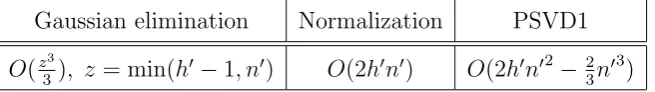
4.1 Required operations for the matrix Ph(κ+1) ∈ Rh0×n0 in the Hybrid
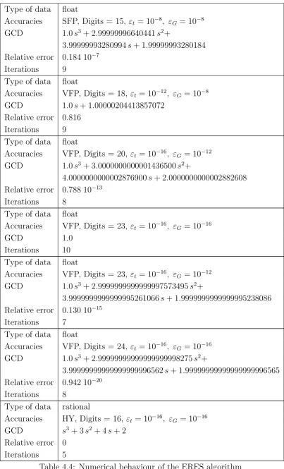
ERES algorithm. . . 91 4.4 Numerical behaviour of the ERES algorithm for the setP11,20 in
Example 4.3. . . 99 4.6 Numerical behaviour of the ERES algorithm for the set P10,9 in
Example 4.4. . . 101 4.7 Storage and time requirements of the ERES algorithm for a random
set of polynomials P12,12. . . 104
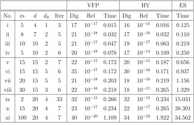
4.8 Behaviour of the ERES algorithm for random sets of polynomials. 104 5.1 Required operations for the computation of the strength bounds. . 118 5.2 The strength of the approximate GCD v(s) = s +c of the set
P ∈Π(3,2; 3) in Example 5.2. . . 123 5.3 Results for theεt-GCD of the set P3,11 in Example 5.5. . . 133
5.4 Results from H-ERES and N-ERES algorithms for randomly se-lected sets of polynomials. . . 136 5.5 Results from the H-ERES algorithm in 16 digits of accuracy. . . . 136 5.6 Comparison of GCD algorithms with randomly selected sets of 10
polynomials: εt = 10−16, Dig = 32 . . . 137
5.7 Comparison of GCD algorithms with randomly selected sets of many polynomials: εt= 10−16, Dig = 32 . . . 138
6.1 Results for the approximate LCM of the set P3 in Example 6.5
given by different least-squares methods. . . 174 6.2 Numerical difference between the result from the S-R LCM and
Hybrid LCM algorithms for the setP0
3 in Example 6.5. . . 175
List of Figures
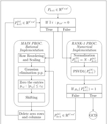
4.1 The Hybrid ERES Algorithm . . . 85
5.1 The notion of the “approximate GCD”. . . 113 5.2 Measuring the strength of a 1st degree approximate GCD of the
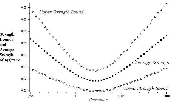
setP ∈Π(3,2; 3) in Example 5.2. . . 123 5.3 Graphical representation of the upper strength bound of v(s) in
Example 5.2. . . 124 5.4 Graphical representation of the lower strength bound of v(s) in
Example 5.2. . . 125 5.5 Graphical representation of the average strengthSa
v(c) of the
com-mon factor v(s) =s+c of the setP in Example 5.3. . . 128 6.1 LCM degrees of the polynomial setP in Example 6.6. . . 179 6.2 LCM residuals of the polynomial setP in Example 6.6. . . 179 7.1 Comparison of the numerical complexity of the RH-ERES algorithm
Acknowledgements
I would like to express my sincerest gratitude to my supervisor, Professor Nicos Karcanias, who supported me throughout my thesis with his friendliness, patience and careful guidance, and shared with me his invaluable knowledge and expertise in the area of Approximate Algebraic Computations. I feel very fortunate to have had the opportunity to be one of his students.
I would also like to show my gratitude to Dr. Marilena Mitrouli, who gave me the first directions to my research, and helped me to stay focused on it. It was her encouragement, persistence, understanding and kindness that I decided to apply for doctoral training, after completing my master’s degree under her supervision.
I would like to thank Dr. Stavros Fatouros and Dr. Dimitrios Triantafyllou for sharing with me their knowledge and their personal work on specific topics of my thesis, and above all for the friendship they offered me, and our excellent cooperation we had over the previous time.
I also thank Prof. George Halikias and Prof. Eric Rogers for their valuable suggestions and remarks which helped me to improve the thesis.
I would also like to thank my closest friends for helping me get through the difficult times, and for all the emotional support and caring they provided.
Lastly, and most importantly, I wish to thank my parents, who raised me, loved me, and supported me, and a special thanks goes to my beloved sister, Vicky Christou, for her love and encouragement to complete my doctoral studies.
Abstract
The area of approximate algebraic computations is a fast growing area in modern computer algebra which has attracted many researchers in recent years. Amongst the various algebraic computations, the computation of the Greatest Common Divisor (GCD) and the Least Common Multiple (LCM) of a set of polynomials are challenging problems that arise from several applications in applied mathematics and engineering. Several methods have been proposed for the computation of the GCD of polynomials using tools and notions either from linear algebra or linear systems theory. Amongst these, a matrix-based method which relies on the properties of the GCD as an invariant of the original set of polynomials under elementary row transformations and shifting elements in the rows of a matrix, shows interesting properties in relation to the problem of the GCD of sets of many polynomials. These transformations are referred to as Extended-Row-Equivalence and Shifting (ERES) operations and their iterative application to a basis matrix, which is formed directly from the coefficients of the given polynomials, formulates the ERES method for the computation of the GCD of polynomials and establishes the basic principles of the ERES methodology.
The main objective of the present thesis concerns the improvement of the ERES methodology and its use for the efficient computation of the GCD and LCM of sets of several univariate polynomials with parameter uncertainty, as well as the extension of its application to other related algebraic problems.
nou dè eÈ toÜ âlssonoc pä toÜ meÐzonoc, ân å leipìmenoc mhdèpote katametr¬ tän prä áautoÜ, éwc oÕ leifj¬ monc, oÉ âx rq¨c prÀtoi präc l-l louc êsontai.}
Two unequal numbers being set out, and the less being continually subtracted in turn from the greater, if the number which is left never mea-sures the one before it until an unit is left, the original numbers will be prime to one another. Antenaresis (Euclidean Algorithm)
Chapter 1
Introduction
Algebraic and geometric invariants are instrumental in describing system properties and characterising the solvability of Control Theory problems [38, 65, 82]. These invariants are defined on rational, polynomial matrices and matrix pencils under different transformation groups (coordinate, compensation, feedback type) and their computation relies on algebraic algorithms, whereas symbolic tools are used for their implementation.
The different type of invariants and system properties defined on a family of linear system models may be classified to those which are generic and those which are nongeneric [46, 82]. Notions such as multivariable zeros of nonsquare systems and decoupling zeros [38] are nongeneric, whereas for square systems, the notion of zeros is generic. Notions such as minimal indices (of various types), are always defined, but they have certain generic values. In dealing with engineering system models, on the one hand the uncertainty about the true value of the parameters, and on the other hand the rounding off computational errors, makes the computation of nongeneric values of invariants a difficult task.
Engineering models are not exact and they are always characterised by param-eter uncertainty. This introduces some considerable problems with any framework based on exact symbolic tools, given that the underlined models are always char-acterised by parameter uncertainty. The central challenge is the transformation of algebraic notions to an appropriate analytic setup within which meaningful
approximate solutions to exact algebraic problems may be sought. This motivates the need for transforming the algebraic problems into equivalent linear algebra problems and then develop approximate algebraic computations, which are ap-propriate for the case of computations on models characterised by parameter uncertainty.
Computing, or evaluating nongeneric types, or values of invariants and thus associated system properties on models with numerical inaccuracies is crucial for applications. For such cases, symbolic tools fail, since they almost always
the value property on the set of models under consideration. The formulation of a methodology for robust computation of nongeneric algebraic invariants, or nongeneric values of generic ones, has as prerequisites:
a) The development of a numerical linear algebra characterisation of the in-variants, which may allow the measurement of degree of presence of the property on every point of the parameter set.
b) The development of special numerical tools, which avoid the introduction of additional errors.
c) The formulation of appropriate criteria which allow the termination of algorithms at certain steps and the definition of meaningful approximate solutions to the algebraic computation problem.
It is clear that the formulation of the algebraic problem as an equivalent numerical linear algebra problem, is essential in transforming concepts of an algebraic nature to equivalent concepts of an analytic character and thus set up the right framework for approximations. This property is referred to asnumerical reducibility (NR) of the algebraic computation and it depends on the nature of the particular invariant.
Given that any set of engineering data has a given numerical accuracy it is clear that there is no point in trying to compute with greater accuracy than that of the original data and thus, an approximate solution has to be sought at some stage, before the procedure converges to some meaningless generic value. In fact, engineering computations are defined not on a single model of a systemS, but on a ball of system models Σ(S0, r(ε)), where S0 is a nominal system andr(ε) is some
radius defined by the data error order ε. The result of computations has thus to be representative for the family Σ(S0, r(ε)) and not just the particular element
of this family. From this viewpoint, symbolic computations carried out on an element of the Σ(S0, r(ε)) family may lead to results, which do reveal the desired
properties of the family. Numerical computations have to stop, when we reach the original data accuracy and an approximate solution to the computational task has to be given.
I Nongeneric Computations
Numerical computations dealing with the derivation of an approximate value of a property, function, which is nongeneric on a given model set, will be called
nongeneric computations (NG). If the value of a function always exists on every element of the model set and depends continuously on the model parameters, then the computations leading to the determination of such values will be called
called generic (GC). For instance, on a set of polynomials with coefficients taking values from a certain parameter set, the greatest common divisor (GCD) has in general the trivial value, equal to 1, and the existence of a nontrivial GCD is a nongeneric computation. On the contrary, the existence of the least common multiple (LCM) is considered generic, since it always exists, given by the product of all the polynomials of the set. Numerical procedures that aim to produce an approximate nontrivial value by exploring the numerical properties of the parameter set are typical examples of NG computations. The computation of nongeneric invariants is linked to nongeneric computations [46].
A number of important invariants for linear systems rely on the notion of the greatest common divisor of several polynomials. The link between control theory and the GCD problem is very strong; in fact, the GCD is instrumental in defining system notions such as zeros, decoupling zeros, zeros at infinity, notions of minimality of system representations and others. On the other hand, systems and control methods provide concepts and tools which enable the development of new computational procedures for GCD. An integral part of the derivation of the procedures for nongeneric computations is the relaxation of certain algebraic definitions, and their embedding in an analytical setup. Appropriate tools have to be devised to indicate degree of presence, or distance from strong possession of a certain property. In such cases, for example the computation of the GCD or the zeros of nonsquare systems, the attention has to be focused on the appropriate termination of the computational algorithm that will allow the estimation of the approximate solutions. The accuracy of the original data determines the threshold, where an algorithm has to terminate and give an approximate solution and where it has to continue.
The definition of theapproximate GCD can be considered as a distance problem in a projective space. The distance framework given for the approximate GCD [22, 42] provides the means for computing optimal solutions, as well as evaluating the strength of ad-hoc approximations derived from different algorithms.
Various methods and algorithms for the computation of the approximate GCD of polynomials have been proposed so far. Many of them rely on Euclid’s algorithm, which is the oldest well-known method for computing the GCD of integer numbers [11, 12, 61, 69, 70]. Other newer methods make use of subresultant matrices [5, 17, 20, 22, 73], perform optimizations and quadratic programming [16, 17, 52], use Pad´e approximations and approximations of polynomial zeros [63] or matrix pencils [45, 49]. Such algorithms usually consist of several different algebraic procedures with a specific task. These algebraic procedures have to be organised properly either in sequential or in iterative way in order to produce the best possible results for the problem that the algorithm is designed to solve. However, the implementation of such algorithms in an appropriate programming environment is not trivial and requires careful selection of data structures and arithmetic system.
I Hybrid Computations
In conventional computer algebra, the usual aim is to perform algebraic computa-tion exactly using racomputa-tional number arithmetic and the introduccomputa-tion of algebraic and transcendental numbers. But many problems coming from areas like com-puter vision, robotics, computational biology, physics etc, are described with inexact numbers (“empirical” numbers) as the input parameters or coefficients. In this context, the usual exact algorithms of computer algebra may not be easily applicable, or may be inefficient. Recent years have witnessed the emergence of new research combining symbolic and numeric computations and leading to new kinds of algorithms, involving algebraic computations with approximate numeric arithmetic, such as floating-point number arithmetic. This combination gives a different perspective in the way to implement an algorithm and introduces the notion ofhybrid computations.
Hybridity refers in its most basic sense to mixture; a mixture of different ways, components, methods etc, which can produce the same or similar results. The basic idea of making something “hybrid” is to improve on its characteristics and therefore make it work better. In our case, we focus on the mixture of symbolic arithmetic and numeric arithmetic, which will be referred to as hybrid arithmetic.
In a hybrid arithmetic system both exact symbolic and numeric finite precision arithmetic operations can be carried out simultaneously. Symbolic computations
which involve only numerical data in rational format, are also referred to as
rational computations and they are always performed in almost infinite accuracy, depending on the symbolic kernel of the programming environment. On the other hand, numerical computations refer to arithmetic operations with numbers in floating-point format (decimal numbers). However, the accuracy of the performed numerical computations is limited to a specific number of decimal digits which gives rise to numerical rounding errors that often cause serious complications and must be avoided [81]. Therefore, the different algebraic procedures, which form an algorithm, can be implemented independently either using symbolic computations or numerical computations. Such kind of implementation will be referred to as
hybrid implementation and hence, the algorithm that is implemented by using symbolic-numeric computations, i.e. hybrid computations, will be called ahybrid algorithm.
The hybridisation of an algorithm (i.e. the hybrid implementation of an algo-rithm) is possible in software programming environments with symbolic-numeric arithmetic capabilities such as Maple, Mathematica, Matlab and others which involve an efficient combination of symbolic (rational) and numerical (floating-point) operations. However, the effective combination of symbolic and numerical operations depends on the nature of an algebraic method and the proper handling of the input data either as rational or floating-point numbers.
Using hybrid computations is basically a trade-off between accuracy and processing time. Symbolic processing always produce exact results and thus it is often used to improve on the conditioning of the input data, or to handle a numerically ill-conditioned subproblem. However, symbolic computations can be very demanding in respect of computational time and data storage, especially in case of large amounts of data. On the other hand, numerical processing is faster and, generally, consumes less computer memory, but the accuracy of the results may not be satisfactory. Therefore, numerical computations are preferable in accelerating certain parts of an algorithm, or in computing approximate outputs. These remarks can be considered as rough guidelines in designing and implementing a hybrid algorithm, but it is not clear how to developthe hybrid algorithm which is capable of giving the best possible results to the problem that is expected to handle. In practise, an effective hybridisation must lead to an algorithm which is fast and accurate (depending on the accuracy of the input data). Therefore, the amount of initial data, the structure of algebraic procedures (sequential or iterative), and the desired level of accuracy are very important factors to be taken into account for the development of an effective hybrid algorithm.
solution, but exact symbolic operations are very expensive regarding computational time and computer memory. This problem is more obvious in matrix-based methods, especially in resultant based methods when the processed matrix is large and dense. On the other hand, numerical finite precision operations are fast and more preferable when an approximate solution is sought. Yet again, the accumulation of numerical errors, especially in iterative methods, can be awfully disastrous.
Amongst the various methods for the computation of an approximate GCD, the ERES [40, 57] is a matrix-based method that can handle sets of several polynomials and allows the development of an effective hybrid algorithm. The ERES is based on the invariance of the GCD under elementary row transformations and involves some basic algebraic procedures, such as Gaussian elimination with partial pivoting and Singular Value Decomposition, which can be implemented separately by using either exact symbolic operations or numerical floating-point operations combined in an optimal setup. The simple structure, the iterative nature and the ability to manipulate large amounts of data are advantages that put the ERES method at the centre of our study for the approximate GCD problem.
I Objectives
The main objectives of this thesis are:
1. To use the basic principles of the ERES method [40, 57] for defining approxi-mate solutions to the GCD problem by developing the hybrid implementation of this method.
2. To use the recently developed framework for defining theapproximate notions
for the GCD as a distance problem in a projective space [42] to develop an optimization algorithm for evaluating the strength of different ad-hoc approximations derived from different algorithms.
3. To improve the context of the ERES methodology and extend its use to other related problems such as the computation of the approximate LCM of sets of polynomials, the evaluation of stability of linear systems and the representation of continued fractions.
The fundamental problems, which relate to the main objectives, are the algebraic representation of the GCD of several polynomials in terms of ERES operations and the investigation of the related problems, such as the matrix representation of the Shifting operation and the matrix representation of the remainder of Euclid’s division algorithm.
and serves as a motivator for the algebraic computational problems involving rational expressions, which are considered in the thesis.
Chapter 3 provides a theoretical presentation of the ERES method. This involves the theoretical issues of the processes involved, such as the selection of an appropriate basis matrix and the application of elementary row transformations, and shifting. The Shifting operation, applied to a matrix, is a key element in the algebraic representation of the whole ERES method. The presented theoretical algebraic procedure of representing the Shifting operation as a matrix product relies on the rank properties of the processed matrix and binds together the iterative steps of the method. This allows the formulation of a new matrix representation for the GCD of a set of several polynomials. The developed framework of the Shifting operation is also used to obtain an algebraic expression for the remainder of the division of two polynomials which evidently establishes a new procedure of polynomial division by using ERES operations.
In chapter 4, the numerical implementation of the ERES method in a symbolic-numeric programming environment is presented. The new ERES algorithm, referred to as Hybrid ERES algorithm, combines in an optimal setup the symbolical application of rows transformations and shifting, and the numerical computation of an appropriate termination criterion, which can provide the required approximate solutions. The termination criterion of the algorithm relies on the partial singular value decomposition method [75, 76]. A new variation of this method is specially developed for the Hybrid ERES algorithm, resulting in a dramatical improvement of its computational performance in the case of large sets of polynomials. The concept behind this method is that, in general, the ERES algorithm terminates when a matrix with rank equal to 1 is obtained. Thus, only the unique singular value and its right singular vector are necessary to be computed. The numerical behaviour of the Hybrid ERES algorithm is also discussed.
Chapter 5 starts with an overview of the fundamentals of the approximate GCD evaluation framework [21, 22, 42]. For sets of polynomials for a given number of elements and with fixed the two maximal degrees, a point in the projective space is defined, based on the coefficients of the polynomials in the set. The family of all sets, which have a GCD with a given degree, is defined by the properties of the generalised resultant and it is shown to be a special variety of the projective space referred to as the d-GCD variety. The factorisation of the resultant has allowed the definition of any d-degree approximate GCD as a subvariety of thed-GCD variety. Thus, thestrength of the approximation, provided by the result of a given numerical method, may be completed as the evaluation of the distance of the given point (set of polynomials) from its subvariety of the
computation of the distance of the given set from thed-GCD variety. This distance is computed by minimising the Frobenius norm of the resultant characterising the dynamic perturbations. The numerical properties of this minimization problem are considered here from a different point of view. Such optimization problems are often non-convex and a reliable solution is not guaranteed. Alternatively, useful information can be obtained by computing some tight bounds for the strength. An algorithm for computing the strength bounds is presented in this chapter. Its main characteristic is that it exploits the properties of resultant matrices in order to produce meaningful results without using optimisation routines and allows the computation of an average strength. These bounds work as indicators, which characterise the quality of a given approximate GCD. The combination of the Hybrid ERES algorithm and the algorithm of strength bounds suggests a complete procedure for the computation and evaluation of an approximate GCD of a set of several polynomials.
The main objective in chapter 6 is to investigate the problem of defining a numerical procedure for the computation of the LCM of a set of several polynomials avoiding root finding and GCD computation. The developed methodologies depend on the proper transformation of the LCM computations to real matrix computations and thus also introduce a notion ofapproximate LCM when working on data with numerical inaccuracies. It is the aim of this chapter to give an alternative new way to compute the LCM of a set of several polynomials based on the ERES method. Two approaches are discussed. The first approach aims at the reduction of the computation of the LCM to an equivalent problem where the computation of GCD is an important part [47], and the second refers to the direct use of Euclid’s division algorithm by ERES operations where there is no need to compute the GCD and the LCM is finally computed by solving an appropriate least-squares problem. The developed algorithms, which are based on these two methods for the computation of the LCM of several polynomials, are implemented in a symbolic-numeric computational environment and their numerical complexity and performance is analysed.
Finally, chapter 8 summarises the achievements and describes issues related to future research. Furthermore, the algorithms, which are presented in this thesis, are implemented in the software computational environment of Maple by using Maple’s programming code and they are listed in the Appendix A.
1.1
Notation
In the following, N, Z, Q, R and C denote the sets (fields) of natural, integer, rational, real and complex numbers, respectively. The imaginary unit in the set of complex numbers is denoted by i. R[s] denotes the ring of polynomials in one variable over R. Capital letters denote matrices and small underlined letters denote vectors. Capital letters followed by a variables∈R denote rational functions ofs or polynomial matrices. Small letters followed by a variable s∈R
denote real polynomials ofs. The following list includes the basic notations that are used in the document.
A∈Rµ×ν Matrix A with elements from
R arranged inµ rows andν
columns (µ, ν ∈N and µ, ν ≥2).
v ∈Rµ Column vector with µ≥2 elements from
R.
At Transpose matrix of A.
vt Transpose vector of v.
ρ(A) or rank(A) The rank of a matrix A.
det(A) The determinant of a square matrix A, (µ=ν).
tr(A) The trace of a square matrix A, (µ=ν) : tr(A) =Pν1=1aii
p(s)∈R[s] A polynomial in one variable s and coefficients in R. deg{p(s)} The degree of a polynomial p(s).
kvk2 The Euclidean norm of v : kvk2 =
pPµ i=1|vi|2
kAk2 The Euclidean norm of A : kAk2 =
√
max eigenvalue ofAtA
kAkF The Frobenius norm of A : kAkF =
qPµ
j=1
Pν
kAk∞ The infinity norm ofA : kAk∞ = max1≤i≤µ Pν
j=1|aij|
dim{ } The dimension of a vector space.
O(k) The highest term in the value equal to O(k) is of order k.
, Mathematical operator which denotes equality by definition.
:= Mathematical operator which denotes equality by input (particularly used in algorithms).
≈ Mathematical operator which denotes approximate equality.
u The machine’s precision (hardware precision). For a t-digit arithmetic system u≈0.5·101−t.
We are mainly concerned here with sets ofm polynomials (m∈N, m≥2) in one variable (univariate polynomials) and coefficients in R, denoted by
Pm,n = n
pi(s)∈R[s], i= 1,2, . . . , m with n= max
i (deg{pi(s)} ≥1) o
(1.1)
Whenever we want to denote the number of elements and the maximal degree of a polynomial set we shall use the notation (1.1). Otherwise the set of polynomials will be abbreviated as P. In the special case where we want to denote that the given set of polynomials Pm,n has at least one monic polynomial with maximum
degree equal ton, we shall use the notationPh+1,n , (i.e.m =h+ 1). The greatest
common divisor and the least common multiple of the setPm,n will be denoted as
Chapter 2
Principles and methods of
algebraic computations
2.1
Introduction
The area of approximate algebraic computations is a fast growing area which has attracted the interest of many researchers in recent years. Two well known problems of algebraic computations are the computation of the Greatest Common Divisor (GCD) and the computation of the Least Common Multiple (LCM) of sets of polynomials. Both of them have widespread applications in several branches of control theory, matrix theory or network theory.
A number of important invariants for linear systems rely on the notion of GCD of many polynomials and, in fact, the GCD is instrumental in defining system notions such as zeros, decoupling zeros, zeros at infinity, notions of minimality of system representations etc. On the other hand, systems and control methods provide concepts and tools which enable the development of new computational procedures for the GCD. The GCD and LCM problems are naturally interlinked [46], but they are of different nature. From the applications in control theory viewpoint, the GCD is linked with the characterisation of zeros of representation whereas LCM is connected with the derivation of minimal representations of rational models. The existence of a common divisor or a common factor of poly-nomials is a property that holds for specific sets and it is not true generically. For randomly selected polynomials, the existence of a nontrivial GCD is a nongeneric property [60], but the corresponding LCM always exists. Therefore, extra care is needed in the development of efficient numerical algorithms calculating correctly the required GCD and LCM.
univariate polynomials in a finite precision arithmetic system, are summarised and the fundamental problems related to the present research are considered.
2.2
Fundamental concepts and definitions
The most basic concept in our study is the polynomial. In simple terms, a polynomial is an algebraic expression of finite length constructed from variables and constants (also known as coefficients), using only the operations of addition, subtraction, multiplication, and non-negative integer exponents. A polynomial of the form:
a(s) =ansn+an−1sn−1+. . .+a1s+a0 (2.1)
with n ∈ N and a0, a1, . . . , an ∈ F, is a polynomial in one variable (univariate)
with coefficients in F, where F can be one of the common fields R, Zor Q. The maximum exponent n for which an 6= 0 is called the degree of the polynomial
and is denoted by deg{a(s)}. If n = 0, then a(s) is a constant polynomial. If
an= 1 the polynomial a(s) is called monic. The set of all univariate polynomials
with coefficients in F together with the two basic operations of addition and multiplication forms the polynomial ring F[s].
In algebra of polynomials, one major property isdivisibility among polynomials. Ifa(s) and b(s) are polynomials in F[s], it is said thata(s) divides b(s) or a(s) is a divisor of b(s) and we write a(s)|b(s), if there exists a polynomial q(s) inF[s] such that:
a(s)·q(s) =b(s) (2.2) Every element in F that zeros a polynomial is called a root (or zero). It is easy to show that every root gives rise to a linear divisor, i.e. ifa(s)∈F[s] and
c∈F such that a(c) = 0, then the polynomial q(s) =s−c divides a(s).
Those polynomials which cannot be factorised into the product of two non constant polynomials are called prime polynomials, or irreducible polynomials. However, any polynomial may be factorised into the product of a constant by a product of irreducible polynomials.
The greatest common divisor (GCD) of a(s) and b(s) is a monic polynomial
g(s) , gcd{a, b} of highest degree such that g(s) is a divisor of a(s) and of
b(s), whilst the least common multiple (LCM) of a(s) and b(s) is a polynomial
l(s),lcm{a, b}of lowest degree such that botha(s) andb(s) dividel(s). The next equation describes the association between GCD and LCM of two polynomials:
Consequently, ifa(s) and b(s) are coprime, then
lcm{a, b}=a(s)·b(s)
Theorem 2.1 ([35]). IfF is a field anda(s) and b(s)are polynomials in F[s]with b(s)6= 0, then there exist unique polynomials q(s), r(s)∈F[s] with
deg{r(s)}<deg{q(s)}<deg{a(s)}
such that
a(s) =b(s)·q(s) +r(s) (2.4) The above theorem refers to Euclidean division, which is also known as
polynomial long division, and shows that the ring F[s] is a Euclidean domain [35]. The polynomialq(s) is called thequotient andr(s) is the remainder of the division, whilst a(s) is the dividend and b(s) is the divisor. Euclid’s division algorithm (or
Euclidean algorithm) is an effective iterative procedure for computing the GCD of a pair of polynomials{a(s), b(s)}, based on the identity (2.4).
The Euclidean algorithm
1. Set i:= 1. Leta(1)(s) :=a(s) and b(1)(s) :=b(s).
2. Use the identity (2.4) and find polynomials q(i)(s),r(i)(s) with
deg{r(i)(s)}<deg{b(i)} such that a(i)(s) =b(i)(s)·q(i)(s) +r(i)(s).
3. If r(i)(s) = 0 then stop; b(i)(s) is a greatest common divisor.
4. If r(i)(s)= 0 then replace6 a(i)(s) by b(i)(s) and b(i)(s) by r(i)(s). Set i:=i+ 1 and go to step 2.
When the GCD is known, the LCM can be determined from the identity (2.3).
REMARK 2.1. In the following we assume that F:=Rand a polynomial of the form (2.1) with coefficients in Rwill be referred to as a real polynomial.
I Representation of polynomials
A real polynomial a(s) may also be represented in vector form as:
a(s) = [a0, a1, . . . , an−1, an]·en(s) (2.5)
wherea= [a0, a1, . . . , an−1, an]t ∈Rn+1 is avector representativeof the polynomial
a(s) and en(s) = [1, s, . . . , sn−1, sn]t. Equivalently, a(s) can be represented as:
where a= [an, an−1, . . . , a1, a0]
t
∈Rn+1 and e0
n(s) = [sn, sn−1, . . . , s,1]t.
However, in most GCD methods the representation of a real polynomial relies on squareToeplitz matrices or companion matrices which provide the means to formulate a representation in matrix terms of the standard factorization of the GCD of a set of polynomials [22, 59].
Toeplitz matrix. The Toeplitz matrix of order n associated to the polynomial
a(s) of degree n is the (n+ 1)×(n+ 1) matrix of the form:
Ta=
a0 0 0 . . . 0
a1 a0 0 . . . 0
..
. . .. ... ...
an−1 an−2 . . . a0 0 an an−1 . . . a1 a0
Companion matrix. Suppose a(s) is a monic polynomial (i.e. an = 1). The
companion matrix associated to the monic polynomial a(s) of degree n is the
n×n matrix of the form:
Ca =
0 0 . . . 0 −a0
1 0 . . . 0 −a1
0 1 . . . 0 −a2
..
. ... . .. ... ... 0 0 . . . 1 −an−1
In some cases, the transpose of Ca can be also considered as companion matrix of
a(s).
I Representation of sets of polynomials
We consider now a set of several real polynomials of the form:
Pm,n = n
pi(s)∈R[s], i= 1,2, . . . , m with n= max
i (deg{pi(s)})≥1 o
(2.7)
wherepi(s) =ai,0+ai,1s+. . .+ai,n−1sn−1+ai,nsn, andai,n6= 0. Each polynomial
pi(s) has a vector representative of the form:
p
i = [ai,0, ai,1, . . . , ai,n−1, ai,n] t
∈Rn+1 , i= 1,2, . . . , m
and therefore the setPm,n may be associated with a vector set:
Pm,n = n
p
i ∈R
Definition 2.1. A basis (or base) of a vector set V is a set B ⊆ V of linearly independent vectors that, in a linear combination, can represent every vector ofV.
In general, a vector set may have several different bases and there are several different algebraic methods which determine various types of bases for a given set of vectors (or a vector space) [18, 35]. Finding an appropriate basis for the vector set Pm,n is an important issue that affects the performance of a GCD or LCM
computational method.
The vector set Pm,n has a direct matrix representation of the form:
Pm = h
p
1, p2, . . . , pm it
=
a1,0 . . . a1,n
..
. . .. ...
am,0 . . . am,n
∈Rm×(n+1)
A polynomial vector p(s) = [p1(s), p1(s), . . . , pm(s)]t may always be associated
with the set Pm,n and this vector can be written in the form:
p(s) = Pm·en(s)
For the set Pm,n the polynomial vector p(s) is a vector representative and the
matrixPm will be called the direct basis matrix of the polynomial setPm,n, which
is formed directly from the coefficients of the polynomials without transformations. (Throughout this thesis,Pm will simply be referred to as “basis matrix”.)
The formulation of an appropriate matrix for the representation of a given a set of polynomials Pm,n is crucial for the development of an efficient matrix-based
method for computing the GCD or LCM of the set. A broad class of GCD methods relies on matrices with special structure. Sylvester and B´ezout matrices are the most common types of matrices which are used in several GCD methods, where procedures for the computation of the rank and nullity of these matrices are essential parts.
Definition 2.2. LetA be an m×n real matrix.
i) The subspace spanned by the row vectors of A is called the row space of
A. The subspace spanned by the column vectors of A is called the column space of A.
ii) The rank of A, denoted by ρ(A), is the dimension of the column space of
A. The matrix is said to have full rank, if ρ(A) = min{m, n}. Otherwise it isrank deficient. A square matrixAn ∈Rn×n isnonsingular, if ρ(An) =n.
Otherwise it is singular.
iii) The space Nr(A) = {v ∈Rn : A v = 0} is called the right nullspace of A.
holdsρ(A) +n(A) =n. Similarly, the space Nl(A) ={u∈Rm :utA= 0}
is called theleft nullspace of A.
For the following definitions let us consider two polynomialsa, b∈R[s] such that:
a(s) = ansn+an−1sn−1+. . .+a1s+a0 , deg{a(s)}=n b(s) = bksk+bk−1sk−1+. . .+b1s+b0 , deg{b(s)}=k
B´ezout matrix. We assume that n =k. The B´ezout matrix (or B´ezoutian) of order n associated to a(s) and b(s) is a n×n matrix obtained as follows:
Bn(a, b) = [ci,j]i,j=1,2,...,n
where each element ci,j is given by
ci,j =
min{i,n+1−j}
X
t=0
aj+t−1bi−t−ai−tbj+t−1
, for i, j = 1,2, . . . , n
The B´ezout matrix of ordern has the next basic properties:
• Bn(a, b) is symmetric as a matrix,
• Bn(a, b) =−Bn(b, a),
• Bn(a, a) = 0,
• Bn(a, b) has full rank if and only if a(s) and b(s) are coprime.
Sylvester matrix. The Sylvester matrix associated to a(s) and b(s) is the (n+k)×(n+k) matrix obtained as follows:
S(a, b) =
an an−1 . . . a1 a0 0 . . . 0
0 an an−1 . . . a1 a0 . . . 0
..
. . .. . .. . .. ... 0 . . . 0 an an−1 . . . a1 a0 bk bk−1 . . . b1 b0 0 . . . 0
0 bk bk−1 . . . b1 b0 . . . 0
..
. . .. . .. . .. ... 0 . . . 0 bk bk−1 . . . b1 b0
k lines n lines
An important property of the Sylvester matrix S(a, b) is that its rankρ S(a, b)
the degree of the GCD of a(s) and b(s), such that:
deg{gcd{a, b}}=n+k−ρ S(a, b) (2.8) The determinant of S(a, b) is called theresultant of a(s) andb(s) and, hence, a Sylvester matrix is also referred to as aresultant matrix. An extended form of the Sylvester matrix for sets of many polynomials is presented in Chapter 5.
2.2.1
Algebraic tools for numerical computations
I Eigenvalues, Characteristic polynomial, and Matrix Pencils
LetA∈Rn×n and I the n×n identity matrix. Then the polynomial
pn(λ) = det(λ I −A), λ∈C
is called the characteristic polynomial of A. The zeros of the characteristic polynomial are called the eigenvalues of A. Equivalently, λ is an eigenvalue of A
if and only if there exists a vector v ∈Rn such that A v= λ v. The vector v is
called a right eigenvector and similarly the vector u∈Rn for which utA=utλ is
called aleft eigenvector. It holds utv = 1.
LetA, B ∈Rn×n, then a linear matrix pencil is the matrix defined as
T(s) = s A−B
for s ∈ R (or s ∈ C). Matrix pencils play an important role in numerical linear algebra. A frequent problem that arises in several algebraic computational methods relates to the computation of the eigenvalues of a matrix pencil. We call eigenvalues of a matrix pencil T(s) all numbers s for which the determinant det(s A−B) = 0. The problem of finding the eigenvalues of a pencil is known as the generalized eigenvalue problem [27] and has numerous applications. A special GCD method, presented in [45, 59], is based on matrix pencil theory.
I Singular value decomposition
The singular value decomposition (SVD) is a special factorisation method for matrices and it is one of the most important methods in numerical linear algebra with a wide range of applications. The development of the theory of the SVD began in the 19th century, but its use became widespread after 1965 when G.
the computation of the inverse or pseudo-inverse of a matrix, and solving linear least-squares problems, or linear systems are some of the problems that the SVD can handle very effectively even when numerical inaccuracies in the data are present [18, 27]. A number of significant properties of the SVD are summarised below.
Definition 2.3. i) An n×n matrix A is said to beinvertible, if there exists a n×n matrix B such that A B =B A =In, where In denotes the n×n
identity matrix. The matrix B is called the inverse of A and it is denoted byA−1.
ii) An n×n matrix is said to be orthogonal, if A At = AtA = In, where At
denotes then×n transpose of A. In this case A−1 =At.
Theorem 2.2 ([18, 27]). Let A be a real m×n matrix (A∈Rm×n). Then, there
always exist orthogonal matrices U ∈Rm×m and V ∈
Rn×n such that
UtA V =
"
Σ1 0
0 0
#
= Σ
where Σ1 ∈ Rr×r is a nonsingular diagonal matrix. The diagonal entries of
Σ∈Rm×n are all non-negative and can be arranged in nonincreasing order. The
number r of non-zero diagonal entries of Σ equals the rank of A.
The decompositionA =UΣVt is known as thesingular value decomposition
ofA. The diagonal entries of Σ are called thesingular values ofAand are denoted by σi, i= 1,2, . . . , r. The columns of U are called left singular vectors and those
of V are called right singular vectors.
The above theorem implies that if r=ρ(A), then there are exactly r positive singular values. These are actually the positive square roots of the nonzero eigenvalues of the matrix AtA (or A At) [27]. If r < min{m, n}, the remaining
singular values are zero. Note that the singular values of a matrix are uniquely determined, but the singular vectors are not unique.
Corollary 2.1. A matrix A∈Rn×n is nonsingular if and only if all its singular
values are different from zero.
The SVD has become an effective tool in handling various important problems arising in a wide variety of application areas, such as control theory, signal and image processing, network theory, pattern recognition, and robotics. Particularly in control theory, the problems requiring the use of SVD include controllability and observability, realisation of state-space models, balancing, robust feedback stabilization, model reduction and several others related problems. Furthermore, the SVD is the most effective tool in solving squares and generalized least-squares problems [25, 28].
I Compound matrices
Compound matrices [56] are useful algebraic tools that are used in certain GCD methods. The following are necessary to describe the notion of compound matrices [46, 59].
a) Qp,ndenotes the set of strictly increasing sequences ofpintegers (1 ≤p≤n)
chosen from 1, . . . , n. The number of the sequences which belong to Qp,n
is np
. If α, β ∈Qp,n we say thatα precedes β (α < β), if there exists an
integer t (1 ≤ t ≤ p) for which α1 = β1, . . . , at−1 = βt−1, αt < βt, where
αi, βi denote the elements of α and β. This describes the lexicographic
ordering of the elements ofQp,n. The set of sequences Qp,n will be assumed
with its sequences lexicographically ordered and the elements of the ordered setQp,n will be denoted by ω.
b) SupposeA= [ai,j]∈Rm×n, letk, pbe positive integers satisfying 1≤k ≤m,
1≤p≤n and letω = (i1, . . . , ik)∈Qk,m and ˜ω= (j1, . . . , jp)∈Qp,n. Then,
A[ω|ω˜]∈Rk×p denotes the submatrix of Awhich contains the rowsi
1, . . . , ik
and the columnsj1, . . . , jp.
c) LetA ∈Rm×n and 1≤p≤min{m, n}, then the pth compound matrix of A
is the mp× np 1
matrix whose entries are ci,j = det{A[ωi−1|ω˜j−1]}, where ωi−1 ∈Qp,m, ˜ωj−1 ∈Qp,n for 1≤i≤ mp
and 1≤j ≤ np
. This matrix will be denoted byCp(A).
I Minors of matrices
Let A be an m×n matrix and p an integer with 0 < p ≤ min{m, n}. A p×p minor of A is the determinant of a p×p matrix obtained from A by deleting
m−prows and n−p columns. Since there are mp 1 ways to choosep rows from
m rows, and there are np 1
ways to choose pcolumns from n columns, there are a total of mp
· n p
minors of size p×p.
1 k p
The (i,j) minor (usually denoted by Mij) of an n×n square matrix A is
defined as the determinant of the (n−1)×(n−1) matrix formed by removing fromA its ith row and jth column. An (i,j) minor Mij is also called the minor of
the element aij of matrix A.
2.2.2
Basic concepts from Linear Systems
We summarise here the fundamentals of linear systems which are essential for describing the work related to GCD and LCM methods that have been developed by using concepts from systems theory [45, 48]. Basic definitions and tools are introduced, related to important properties of linear systems, such as system poles and zeros, controllability, observability, and stability.
A linear system may be represented in terms of first order differential equations as
S(A, B, C, D) : x˙(t) = A x(t) +B u(t)
y(t) = C x(t) +D u(t) (2.9) where the variabletrepresents time,x(t) is thestate vector,u(t) is theinput vector
andy(t) is theoutput vector. The matrices A∈Rn×n,B ∈
Rn×p, C ∈Rm×n, and
D∈Rm×p are the state,input, output, and feedforward matrices, respectively. In
system matrix form, we can represent the system by:
P(s) =
"
s I−A −B
−C −D
#
(2.10)
or by the transfer function model:
G(s) = C(s I −A)−1B+D (2.11) which is an m×p polynomial matrix. The 4-tuple (A, B, C, D) is said to be a
realisation ofG(s). The matrixP(s) is a matrix pencil entirely characterising the state-space model and it is known as the Rosenbrock System Matrix Pencil [65]. For the state-space model S(A, B, C, D) of which is excited by an initial conditionx(0) =x0 and a control input u(t), the corresponding solutions for the
state and output trajectories x(t), y(t) are given by [1] :
x(t) = eAtx0+
Z t
0
eA(t−τ)Bu(τ)dτ (2.12)
y(t) = CeAtx0 +
Z t
0
CeA(t−τ)Bu(τ)dτ+Du(t) (2.13)
of the solutions are obtained:
x(s) = (sI −A)−1x0+ (sI−A)−1Bu(s) (2.14) y(s) = C(sI−A)−1x0+ C(sI−A)−1B+D
u(s) (2.15)
I Controllability, Observability
Let us consider a system S(A, B, C, D) described by the equation (2.9). We say that the system is controllable if given any initial state x(t0) = x0, there exists a
finite time t1 > t0 and a control u(t) defined on t0 ≤t ≤t1, such that x(t1) = 0.
Therefore, controllability refers to the ability of a system to transfer the state fromx0 to the zero state in finite time.
Theorem 2.3 ([1]). The pair (A, B) is controllable, if and only if
rank
B, AB, A2B, . . . , An−1B
=n
The system (2.9) is said to beobservable, if for any statex(t0) =x0 and given
control vector u(t) knowledge of y(t) on t0 ≤ t ≤ t1 is sufficient to determine x0. Therefore, observability means that we can determine the initial state of the
system for a suitable measurement of the output y(t). The notion of observability is dual to that of controllability. Thedual system of (2.9) is defined as the system:
S(At, Ct, Bt, Dt) : x˙d(t) = A
tx
d(t) +Ctud(t)
yd(t) = Btxd(t) +Dtud(t)
(2.16)
Theorem 2.4 ([4]). The system described in (2.9) is observable if and only if its dual system (2.16) is controllable. Thus, the pair (A, B) is observable if and only if the pair (At, Ct) is controllable, that is :
rankCt, AtCt, . . . ,(At)n−1Ct=n
There are tests for controllability and observability that involve the eigenvalues and the eigenvectors of A. These tests are particularly useful both as theoretical and computational tools. We can also check controllability and observability of a system in the following ways [1] :
Rank tests for controllability and observability :
• The pair (A, B) is controllable, if and only if
rank[λ I−A, B]=n
• The eigenvalue λi is an uncontrollable eigenvalue of A, if and only if
rank([λiI−A, B])< n
• The pair (A, B) is observable, if and only if
rank
"
λ I−A C
#!
=n
for all eigenvalues λ of A.
• The eigenvalue λi is an unobservable eigenvalue of A, if and only if
rank
"
λiI −A
C
#!
< n
The uncontrollable, unobservable, uncontrollable and unobservable eigenvalues are also referred to asinput,output, and input-output decoupling zeros (idz,odz,i-odz) [65] and the corresponding sets, including multiplicities, are denoted by
ZID,ZOD, ZIOD, respectively. There exist more definitions of controllability and
observability, which can be found in [1, 38, 50, 65]. Alternative algebraic tests based on the restricted pencils are given in [39].
I Poles and Zeros, Pole and Zero polynomials
Classical control design techniques are based on the concepts ofpoles andzeros
of a rational function. Every rational transfer function can be expressed as a polynomial matrix (i.e. a matrix whose elements are univariate polynomials), divided by a common denominator polynomial. So, every polynomial matrix can be reduced to a canonical form known as the Smith form [24].
Definition 2.4. A polynomial matrix is called unimodular if it has an inverse which is also a polynomial matrix.
There are three elementary operations which can be performed on polynomial matrices:
• Interchange of any two rows, or columns.
• Multiplication of one row or column by a nonzero constant.
• Addition of a polynomial multiple of one row or column to another.
rational) matrices P(s) and Q(s) are equivalent if there exist sequences of left
{L1(s), L2(s), . . . , Ll(s)} and right {R1(s), R2(s), . . . , Rr(s)} elementary matrices
such that
P(s) =L1(s)L2(s) · · · , Ll(s)Q(s)R1(s)R2(s) · · · , Rr(s)
The next result states that every polynomial matrix is equivalent to a diagonal polynomial matrix known as the Smith form [24].
Theorem 2.5. Let P(s) be a polynomial matrix of normal rank r (i.e. of rank r for almost alls). Then, P(s) may be transformed by a sequence of elementary row and column operations into a pseudo-diagonal polynomial matrixPS(s) having the
form:
PS(s) = diag{ε1(s), ε2(s), . . . , εr(s),0, . . . ,0}
in which each εi(r), i= 1,2, . . . , r is a monic polynomial satisfying the divisibility
property εi(s)|εi+1(s) for i = 1,2, . . . , r −1 (i.e. εi(s) divides εi+1(s) without remainder). Moreover, if we define the determinantal divisors
D0(s) = 1
D1(s) = GCD of all i×i minors of P(s) where each GCD is normalised to be a monic polynomial, then
εi(s) =
Di(s)
Di−1(s)
, i= 1,2, . . . , r
The matrixPS(s) is the Smith form ofP(s), and the εi(s)are called the invariant
factors of P(s).
It is clear that the Smith form of a polynomial matrix is uniquely defined, and that two equivalent polynomial matrices have the same Smith form. The Smith form is thus a canonical form for a set of equivalent polynomial matrices. This can be extended to rational matrices [65].
Theorem 2.6. Let G(s) be a rational matrix of normal rank r. Then G(s)
may be transformed by a series of elementary row and column operations into a pseudo-diagonal rational matrix of the form:
M(s) = diag
ε1(s) ψ1(s)
, ε2(s) ψ2(s)
, . . . , εr(s) ψr(s)
,0, . . . ,0
in which the monic polynomials {εi(s), ψi(s)} are coprime for each i and satisfy
the divisibility properties εi(s)|εi+1(s) and ψi+1(s)|ψi(s) for i = 1,2, . . . , r −1.
We now define the poles and zeros of a transfer function matrix by means of the Smith-McMillan form [65].
Definition 2.5. Let G(s) be a rational transfer function matrix with Smith-McMillan formM(s). The pole p(s) and zero z(s) polynomials, respectively, are defined as
p(s) = ψ1(s)ψ2(s)· · ·ψr(s) (2.17)
z(s) = ε1(s)ε2(s)· · ·εr(s) (2.18)
The roots of p(s) andz(s) are called thepoles and zeros of G(s), respectively. In other words, the poles ofG(s) are all the roots of the denominator poly-nomialsψi(s) of the Smith-McMillan form of G(s). Ifp0 is a pole of G(s), then
(s−p0)ν must be a factor of some ψi(s). The number ν (ν ≥ 1) is called the
multiplicity of the pole, and if ν = 1 we say that p0 is a simple pole. Zeros and
their multiplicity are defined similarly, in terms of the numerator polynomials
εi(s) of the Smith-McMillan form.
REMARK 2.2. If G(s) is square, then det(G(s)) = cz(s)
p(s) for some constant c. In this case, although the pair of polynomials {εi(s), ψi(s)} is coprime for each
i = 1,2, . . . , r, it is possible that there exist common factors between p(s) and
z(s) which cancel out in forming det(G(s)).
Definition 2.6. The degree of the pole polynomialp(s) is the McMillan degree
of G(s).
Zeros defined via the Smith-McMillan form are often calledtransmission zeros, in order to distinguish them from other kinds of zeros which have been defined. For a single input, single output (SISO) system represented by a rational transfer function G(s), where G(s) = n(s)
d(s) and n(s), d(s) are coprime polynomials with deg{n(s)}=r and deg{d(s)}=n, we define as finite poles the roots of d(s) and asfinite zeros the zeros of n(s). If r < n we say thatG(s) has an infinite zero of order n−r, and if r > n, then G(s) has a infinite pole with ordern−r.
Poles and zeros are also related to the eigenvalues of the system matrix A. The eigenvalues and eigenvectors of the matrix A define the internal dynamics of the system S(A, B, C, D). For every eigenvalue λ of A we have two eigenvalue-eigenvector problems:
A v = λ v , (2.19)
wtA = wtλ , wtv = 1 (2.20)
{νi, i ∈ q˜⊂ N}, that is the sequence of dimensions of λ-Jordan blocks in the
Jordan form of A. Alternatively, S(λ) is defined by the set of degrees of the (s−λ)ν type of the Smith form of sI−A. ThenPqi=1νi =pis called thealgebraic
multiplicity andq is the geometric multiplicity ofλ. The maximal of all geometric multiplicities of the eigenvalues of A is referred to as the Segre´index of A.
Definition 2.7. The set of eigenvalues of the matrixA, which are the roots of the characteristic polynomial of A, are called the system internal poles, or the system eigenvalues. The roots of the pole polynomial of G(s) are called the external system poles or system poles.
Definition 2.8. The zeros of the system are defined as those frequencies s0 ∈C
for which there exists an inputu(t) =u0es0tsuch that, given zero initial conditions
for the state of the systemx(t), the output y(t) is zero.
The above dynamic characterisation leads to a matrix pencil characterisation of zeros [44]. A linear system may also have poles and zeros at infinity ∞, which indicate thatG(∞) loses rank. Poles are associated with resonance phenomena (explosion of the gain) and zeros are associated with antiresonance phenomena (vanishing of the gain). In this sense, the notions of poles and zeros are dual and it is this basic property that motivates a number of definitions and problems that relate to multivariable poles and zeros [41, 55].
I Internal-External and Total stability
The most important concept and property for any system is that ofstability, which has to do with the behaviour of all trajectories which may be generated for families of initial conditions and control input. For linear, time invariant systems the notions of stability, which are more frequently used are defined next. We consider stability of equilibrium points, whereas stability of motion is always reduced to the previous case. Note that the origin (x= 0) is always an equilibrium point for
S(A, B, C, D) models.
Definition 2.9 ([1]). Given a system of first-order differential equations :
˙
x=F(t, x), x∈Rn
a point xe ∈ Rn is called an equilibrium point of the system (or simply an
equilibrium) at timet0 >0, if F(t, x0) = 0 for all t > t0.
Definition 2.10 ([1]). The state-space model S(A, B, C, D) will be called:
ii) Asymptotically internally stable, if for any initial state x(0) the zero input response remains bounded for all t≥0 and tends to zero ast → ∞. This property will be referred to in short as internal stability (IS).
iii) Bounded Input Bounded Output stable (BIBO), if for any bounded input the zero state output response (x(0) = 0) is bounded.
iv) Totally stable (TS) if for any initial state x(0) and any bounded input u(t), the output, as well as all state variables, are bounded.
The notion of BIBO stability refers to the transfer function description and may also be called as external stability. A number of criteria for these properties, based on eigenvalues-poles, are summarised below.
Theorem 2.7 ([15]). Consider the system S(A, B, C, D)with G(s) transfer func-tion and let {λi =σi+iωi, i∈˜n⊂N}, {pj = ¯σj +iω¯j, j ∈k˜⊂N} be the sets
of eigenvalues, poles respectively. The system has the following properties:
i) Lyapunov internally stable, if and only if σi ≤0, for all i ∈ n˜, and those
with σi = 0 have a simple structure (algebraic multiplicity is equal to the
geometric multiplicity).
ii) Asymptotically internally stable, if and only if σi <0, for all i∈n˜.
iii) BIBO stable, if and only if σ¯j <0, for all j ∈k˜.
iv) Totally stable, if it is Lyapunov internally stable and BIBO stable.
Note that IS implies BIBO-stability and thus TS. BIBO-stability does not always imply IS, since transfer function and state space are not always equivalent. If the two representations are equivalent (when system is both controllable and observable), then BIBO-stability is equivalent to IS and thus TS.
Eigenvalues and poles are indicators of stability. Equivalent tests for stability, without computing the eigenvalues or poles, are defined on the characteristic or pole polynomial by the Routh-Hurwitz conditions [24].
2.2.3
Almost zeros of a set of polynomials
The subject of nongeneric computations has as one of its most important topics the study of almost zeros. A summary of the notion is given next [46]. The computational issues and the feedback significance of the notion (trapping disks for multiparameter root locus) is given in [43]. We consider the setPm,n as defined
When s ∈C, p(s) defines a vector valued analytic function with domain C and co-domainCm; the norm of p(s) is defined as a positive real function with domainC, such that
kp(s)k=
q
pt(s∗)p(s) =pet
n(s∗)Pmt Pmetn(s) (2.21)
where s∗ is the complex conjugate of s. Note, that if q(s) = s−c is a common factor of the polynomials pi(s),i= 1,2, . . . , m, then pi(c) = 0, p(c) = 0 and thus
kp(c)k= 0. This observation leads to the following definition.
Definition 2.11. Let P be a set of polynomials of R[s], p(s) be the vector representative and let φ(σ, ω) = kp(s)k, where s = σ +iω ∈ C. An ordered pair (zk, εk), zk ∈ C, εk ∈ R and εk ≥ 0, defines an almost zero of P at s =zk
and of order εk, if φ(σ, ω) has a minimum at s=zk with value εk. From the set
Z ={(zk, εk), k= 1,2, . . . , r} of almost zeros of P the element (z∗, ε∗) for which
ε∗ = min{εk, k= 1,2, . . . , r} is defined as the prime almost zero of P.
It is clear that ifP has an exact zero, then the correspondingε is zero. Clearly the previous definition is an extension of the concept of exact zero to that of the almost zero. The magnitude ofε at an almost zero s=z provides an indication of how wellz may be considered as an approximate zero of pi. However, that ε
depends on the scaling of the polynomials pi(s) inP by a constant c∈R r{0}.
The general properties of the distribution of the almost zeros of a set of polynomials
P on the complex plane were considered in [43] and are summarized below.
Theorem 2.8. The prime almost zero of P is always within the circle centred at the origin of the complex plane and with radius p∗, defined as the unique positive solution of the equation:
1 +r2 +. . .+r2n = γ
2 γ2 =θ
2
where γ, γ denote the maximum and minimum singular values of Pm, respectively.
The term θ will be referred to as the condition number of P. The disc [0, p∗] within which the prime almost zero lies, is referred to as theprime disc ofP. The following general results may be stated for the radius p∗.
Proposition 2.1. If n is the maximum degree and θ the condition number of P, then the radius p∗ =f(n, θ) of the prime disc is a uniquely defined function of n and θ and it has the following properties:
1. The radius p∗ is invariant under the scaling of the polynomial of P by the same nonzero constant c.