Multiobjective memetic algorithm applied to the optimisation of water distribution systems

Multiobjective Memetic Algorithm Applied

to the Optimisation of Water Distribution Systems

Euan Barlow&Tiku T. Tanyimboh

Received: 4 December 2012 / Accepted: 27 March 2014

#The Author(s) 2014. This article is published with open access at Springerlink.com

Abstract Finding low-cost designs of water distribution systems (WDSs) which satisfy appropriate levels of network performance within a manageable time is a complex problem of increasing importance. A novel multi-objective memetic algorithm (MA) is introduced as a solution method to this type of problem. The MA hybridises a robust genetic algorithm (GA) with a local improvement operator consisting of the classic Hooke and Jeeves direct search method and a cultural learning component. The performance of the MA and the GA on which it is based are compared in the solution of two benchmark WDS problems of increasing size and difficulty. Solutions that are superior to those reported previously in the literature were achieved. The MA is shown to outperform the GA in each case, indicating that this may be a useful tool in the solution of real-world WDS problems. The potential benefits from search space reduction are also demonstrated.

Keywords Penalty-free memetic algorithm . Multi-objective optimisation . Water distribution system design . Parallel computing . High performance computing . Search space reduction

1 Introduction

Water distribution systems (WDSs) are integral components to the effective design of urban areas, and the ever-increasing urbanisation in developed and developing countries world-wide establishes the problem of optimising WDS design as an important research area. These systems are the networks of pipes, pumps, reservoirs, tanks and nodes which transport drinking water from the supply source to the users. The optimal design of WDSs is very challenging. These combinatorial optimization problems have linear objectives, large numbers of non-linear constraints, extremely large discrete solution spaces and multi-modal objective spaces. To enable the optimal design of real-life WDSs an effective solution method which is reliable, easy to implement and computationally efficient is desired. One goal of WDS design among

DOI 10.1007/s11269-014-0608-0

Electronic supplementary material The online version of this article (doi:10.1007/s11269-014-0608-0) contains supplementary material, which is available to authorized users.

E. Barlow

:

Department of Civil and Environmental Engineering, University of Strathclyde, John Anderson Building, 107 Rottenrow, Glasgow G4 0NG, UK

others (Kanakoudis2004; Tanyimboh and Kalungi2009, etc.) is to find the cheapest network configuration which provides an adequate pressure at all user outlets.

Heuristic search techniques are considered ideal tools in solving WDS design optimisation problems and genetic algorithms (GAs) are perhaps the most widely used method (see e.g. Siew and Tanyimboh 2012). However, many alternative heu-ristics techniques have also been applied (see e.g. Bolognesi et al. 2010). Memetic algorithms (MAs) are hybrid methods which combine the powerful explorative search capabilities of heuristic methods with some form of local improvement or exploitation, and these methods are increasingly being applied to real-world optimisation problems. Local improvement methods can effectively converge towards locally optimal solu-tions; however, they have no capacity to identify global optima. A hybrid method which harnesses the exploitation of local improvement with the exploration of GAs therefore has the potential to improve the convergence of a standard GA and reduce the computation time required.

Memetic algorithms have been applied in the solution of least-cost WDS design. Starting with a GA as the heuristic search mechanism, local improvement has been incorporated into the algorithm using machine learning (di Pierro et al.2009), cellular automaton (Guo et al. 2007), linear programming (Cisty2010), integer linear programming (Haghighi et al.2011) and a variety of classical local search techniques (Banos et al.2010). Additionally, hybrid methods such as the shuffled frog leaping algorithm (Eusuff and Lansey2003), scatter search with simulated annealing (Banos et al. 2009), differential evolution (DE) with non-linear programming (NLP) (Zheng et al.2011) and a method combining a classical local search technique with a dynamic dimension reduction technique (Tolson et al.2009) have all been tested on various benchmark problems.

In this paper a multiobjective memetic algorithm is introduced. The MA hybridises a robust GA with local improvement based on the classical Hooke and Jeeves direct search method and a cultural improvement operator. This MA is tested here on the solution of the least-cost WDS design problem.

2 Multi-Objective Formulation of the Least-cost WDS Design Problem

There has been growing recognition of late in the water engineering community that the least-cost design of a WDS is more accurately represented as a multi-objective optimisation problem, where the conflicting objectives are cost and network perfor-mance. The cost, which is to be minimised, covers the capital expenditure required to construct the network. For simplicity, the only cost considered here is the initial capital expenditure; more realistic approaches to costing over the entire lifetime of a network are available in e.g. Skipworth et al. (2002) and Tanyimboh and Kalungi (2008). The network cost is

f₁ð Þ ¼x X

i¼1 NP

c dið ;liÞ ð1Þ

where the cost of a specific pipe is given by the function cwhich is dependent on the length and diameter of theith pipe, NP is the number of pipes in the network andxis

the decision variable vector, to be defined.

straightforward to implement and inexpensive to compute. The total pressure deficit across the network is

f₂ð Þ ¼x X

j¼1 NN

max hrj−hpj;0

ð2Þ

where the required head and the achieved head at nodejarehrj andhpj respectively andNNis

the number of demand nodes. This objective addresses the minimum nodal pressure con-straints

hp_j≥hrj for j¼1;…;NN ð3Þ

The multi-objective least-cost WDS design problem is therefore formally expressed as

min

x∈Ff xð Þ ¼

f1ð Þx;f2

x

T

ð4Þ

wheref1andf2are given by Eqs. (1) and (2) respectively andFis the feasible decision space. By considering the nodal deficits as an objective a WDS designer is able to assess whether the extra cost required to achieve a feasible solution is preferable to a slight shortfall in flow and pressure for a cheaper cost. This is more representative of the real-life situation in designing WDSs. In general, the problem specification for a particular WDS will define the non-linear cost function,c, the length of each pipe,l, and the required head at each node,hr. The decision variables in this formulation are therefore the discrete pipe diameters,x¼ðd1;…;dNPÞT , which control the nodal heads,hp, throughout the network. The problem concerns solving

Eq. (4) subject to the conservation of mass and energy constraints over the set of all feasible (commercially available) pipe-diameters,F. By analysing each network design configuration with a hydraulic solver, satisfaction of the conservation of mass and energy constraints is guaranteed.

3 Memetic Algorithm

A GA is the main optimisation tool which comprises the MA proposed here. GAs are particularly effective in solving multi-objective problems, as the population of solutions provides a natural setting for producing the Pareto-optimal front. The strengths of a GA are well suited to the optimal design of a WDS; however, their stochastic nature can result in slow, unreliable convergence. As the hydraulic evaluation of a WDS requires an external solver, each fitness evaluation is important. For real-life networks that can have hundreds or thousands of pipes the CPU time to evaluate a single candidate solution can be substantial, and the time required to simulate the hydraulic response of millions of candidate solutions over the evolution of a GA could be restrictive. Quick, robust convergence to the optimal solution is therefore extremely desirable.

3.1 Implementation of Local Improvement

The MA proposed here consists of a GA concurrently hybridised with local and cultural improvement operators; the GA operates as normal, except that everyNGgenerations the child

selected according to rank and crowding distance from the child and parent populations. The next generation of parent population is thus formed and the GA continues as normal, where

Npopis the population size. This allows the local and cultural improvement to slot neatly into

the framework of the GA with minimal increase in complexity. The structure of the MA is illustrated in Fig.1.

It is common in the WDS literature to measure a solution by its effectiveness at locating the least-cost zero-deficit, i.e. hydraulically feasible, solution. This solution occupies one extrem-ity of the current non-dominated front, and individuals which reside in this low-deficit region of objective space are more likely to be modified through local improvement to obtain the optimal solution than individuals residing in any other region of objective space. For this reason only a subset of the population which is in some proximity to the cost-effective low-deficit region of the current population will be considered for selection. The subset of the population from which individuals may be selected is denoted by S, and this subset is characterised by the parameterNLS, such thatS comprises the NLS% of individuals in the current non-dominated front with the lowest deficits. At each generation when local improve-ment is to be applied, one member ofSis randomly selected as the starting point for the search. The search then moves to the next individual along the non-dominated front untilNpopchildren

have been created; in this way each implementation will result in a localised area of the front being improved.

3.2 Scalar Assessment of Fitness

Measuring the fitness of a solution generated through local search in a similar manner to the Pareto-based fitness assessment used in a multiobjective GA would require each new solution to be compared with the entire current population using the computationally intensive non-dominated sorting and crowding distance operators. A far more efficient method involves replacing the multi-objective fitness function of Eq. (4) with a surrogate measure which represents an individual’s multi-dimensional fitness vector as a scalar fitness value. The multi-objective problem is thus transformed into a single-objective problem and classical optimisation techniques can then be applied to locally improve a solution. The current state-of-the-art in classical approaches to multi-objective problems employ techniques which utilise surrogate measures (Erfani and Utyuzhnikov2011).

The scalar fitness assessment used here is the standard linear weighting method (Miettinen 1998), where each objective function is scaled by a weighting coefficient and the surrogate objective is to minimise the weighted sum of both objectives. That is,

min

x∈F gð Þ ¼x

X

i

wifið Þx ;

X

i

wi¼1; wi>0;∀i: ð5Þ

in whichwiis the weight associated with theith objective function,fi.

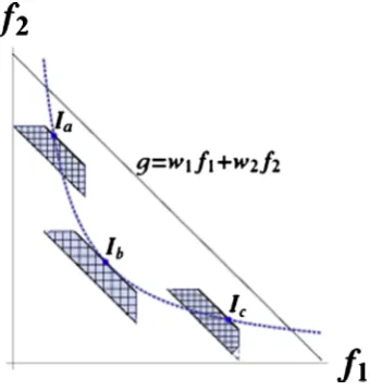
In the two-dimensional objective space of a WDS least-cost design problem, the weighted fitness function (WFF) in Eq. (5) defines a line with a negative gradient which cuts the positive axis of both objective functions, as displayed in Fig. 2. To reduce the value of the fitness functiong, a solution must be found which can focus the search towards the Pareto-optimal front. The effectiveness of the WFF is dependent on the orientation of the linegwith respect to the current non-dominated front; this orientation is defined solely by the weighting co-efficients and appropriate definition of these weights is therefore crucial in conducting a successful local search. The WFF must be locally relevant to the selected individual, which acts as the starting point for the local search, and any improvements with respect to the WFF should coincide with actual improvements to the starting individual or the population as a whole.

Figure2displays a particular WFFgwith fixed weights and a WFF with the same weights intersecting the non-dominated front in a given generation at the location of three solutions or individuals,Ia,IbandIc. At the locations of individualsIaandIc, the WFF cuts through the

front. An individual identified through local search as an improvement could occupy anywhere below the WFF, as indicated by the hatched region at each individual. There is clearly an overlap between the hatched region at each individualIaandIcand the regions of the objective space which are currently dominated, which reduces the effectiveness of this WFF at the locations of these individuals. Figure2also shows that the WFF is almost tangential to the front at the position of individualIb. Any individuals identified through local search which

improve the value of the WFF will also improve the population as a whole. This is clearly a more desirable situation and designing a WFF which approximates the gradient of the current non-dominated front at the location of the starting individual is more effective. A WFF defined

in this way is unable to guarantee a search in a non-dominated region of the objective space if the front is concave at that location; however, in reality the front is discrete and therefore will not be truly concave or convex at any given location.

As the explicit form of the current non-dominated front is not known at a given location, the gradient of the front cannot be analytically determined and a numerical approximation must be utilised. To approximate the gradient of the non-dominated front at a given location, a group of individuals around the chosen location are selected and the gradient of the best-fitting straight line through these individuals is found using a least-squares method. The gradientmaround an individualIiis approximated here by (Berendsen2011)

m¼

X

j¼−NI NI

f₁ Ii_þj

−f¯₁

f₂ Ii_þj

−f¯₂

X

j¼−NI NI

f1 Iiþj

−f¯1

2 ð6Þ

whereIiindicates theith individual along the current non-dominated front,f1(Ii) andf2(Ii) are

the respective objective function values corresponding to individualIiand f1 and f2 are the respective average objective function values for all individuals in this group. We use a sample of 2NI+1 individuals to generate the gradient. The firstNIindividuals are selected in each direction along the current non-dominated front from the position of individualIi. Smaller

groups of individuals will provide a more accurate representation of a gradient local to a given point on the Pareto-front, and this is supported by our investigations. As the 2NI+1 individuals

are mutually non-dominating, it can be shown from Eq. (6) that the gradient mis strictly negative. Defining the weights as

w1¼₁−₋m_m

w₂¼ 1

1−m

ð7Þ

therefore ensures the requirement∑wi=1 in Eq. (5) is satisfied. The multi-objective problem

given by Eq. (4) is thus replaced with the single-objective problem given by Eqs. (5) and (7).

3.3 Single Objective Optimisation

explored and the search moves onto the next stage. When the maximum number of decision variables have been investigated (either the number of decision variables related to the problem or some pre-specified limit), the pattern search step is applied. The difference between the current optimal value for each decision variable and the original decision variable value is calculated. This difference identifies a pattern search direction which improves the original solution over all decision variables. The pattern search direction is then exploited further by performing an additional search in this direction. The process then repeats, performing another univariate search from the current optimal position.

3.4 Cultural Learning

The final component of the MA is cultural learning where a localised group of individ-uals learn from each other what constitutes an improvement. The pattern direction generated from the Hooke and Jeeves operator in Section3.3 constitutes a direction of improvement in decision space, where improvement is measured relatively to the WFF. The WFF defined in Section 3.2 such that it approximates the gradient to the current non-dominated front at a particular location in objective space may also give a close approximation to the gradient of the front at the location of nearby individuals. A group of consecutive individuals along a non-dominated front occupy a similar region of objective space in terms of the relationship between cost and deficit for each individual. To achieve the same balance between cost and deficit, it is likely that an individual will share some combinations of decision variables with its neighbours. A pattern direction for one individual, which identifies a direction of improvement in decision space, may therefore lead to improvements if applied to the neighbouring individuals.

The cultural learning operator is implemented after the local search discussed above has taken place. A group ofNCconcurrent individuals along the non-dominated front, which is centered on the individual selected for local improvement, is selected for cultural learning. It is assumed that the group of concurrent individuals will have enough similarities in decision variables and will be close enough in objective space to the gradient specified by the WFF that this is an appropriate measure of improvement. The pattern direction is therefore applied to each individual in the group to generate new individuals in the child population. This cultural learning step will enable larger regions of objective space to be locally improved per generation, as the Hooke and Jeeves search is only applied to one member of the group. The number of children generated from one group of individuals is therefore less than the number that would be required if the Hooke and Jeeves search was applied to every individual in the group, so more groups of individuals can be improved and larger regions of the non-dominated front can be searched.

4 Results

initiated optimization runs. Also, the MA’s results are compared with the best available solutions in the literature based on various other solution approaches.

4.1 Parallelisation of the Algorithms

In order to improve computation times the operation of the GA and the MA were parallelised. Two separate parallelisation methods were utilised, each designed to address a particular computational burden. In a single optimisation run the large number of network evaluations performed can lead to substantial computation times, particularly for larger problems. In order to speed up the progress of the evolution a controller-worker model was implememented, where the controller performs the routine operation of the algorithm and employs the workers to perform the fitness evaluations. Additionally, an island model was employed so independent optimisation runs are performed simultaneously. This combination yields a series of islands, each performing separate optimisation runs, with a controller-worker architecture between the processors assigned to each island. This combined approach enables substantially more processors to be employed than would be available if either of the parallelisation models were used alone. To perform the optimisation runs the high-performance computer at the University of Strathclyde (HPCUOS) was used. This facility has 1048 cores, each with 2.93 GHz CPU and 12 GB RAM. A range of cores from 16 to 160 was utilised, depending on the requirements of a particular optimisation. The benefits of this parallelisation are that an optimisation which would have taken approximately 160 days with a single processor on a workstation with 2 quad-core 2.27 GHz processors and 12 GB RAM was perfomed in just over 1 day, a reduction of over 99 %.

4.2 Baseline GA

We used the Pareto-based elitist multiobjective genetic algorithm NSGA II (Deb et al.2002) as the baseline GA upon which the MA is constructed. The framework of the MA given in Section3is designed to be simple to implement and complimentary with any GA. Hence any alternative GA could be used. The decision variables are integer-coded, where each integer represents a specific pipe-size. One-point crossover is applied to generate two children from a pair of parents derived from a randomly populated binary tournament. Mutation is applied to each decision variable of each child with a probability ofpm. If a particular decision variable is

selected for mutation, then, either a random mutation, where a new value is selected at random, or a creeping mutation is applied, where either the next larger or next smaller value is selected, each with a conditional probability of 0.5. If the decision variable is equal to a boundary value, the feasible adjacent value is selected with a conditional probability of 1. Both random and creeping mutation are applied with a conditional probability of 0.5 each.

4.3 Parameter Values

The parameter values which are used throughout the Results section are as follows: probability of crossover,pc=1; probability of mutation,pm=1/Np;Npis the number of decision variables

or pipes in each problem; population size,Npop=200 (Kadu network) andNpop=500 (Balerma

network); frequency of applying local and cultural improvement operators,NG=10; number of

individuals to generate the WFF,NI=1; number of concurrent individuals selected for cultural

improvement, NC=4; percentage of non-dominated front available for local improvement,

the least-cost solution for the Balerma network to date used a population size of 500 also. A preliminary sensitivity analysis was performed on each parameter: first the GA parameters were investigated and a combination of good parameter values were found. The same values were then used for the MA and the additional MA parameters were then investigated. The values used here were found to perform well collectively, however, it may be that different combinations of these parameter values provide comparable or even better results–this is an area of ongoing investigations. The respective network-specific design data can be found in Kadu et al. (2008) and Reca and Martinez (2006).

4.4 Kadu et al. (2008) Network

The WDS consists of two reservoirs, 26 nodes and 34 pipes. There are 14 discrete pipe sizes giving a solution space of 1434or almost 1039design configurations. The cheapest solution previously found to this problem is Rs131.31×106(Haghighi et al.2011) with the Hazen– Wiliams formula ashf=ωl(Q/C)1.85d-4.87wherehf=headloss;ω=coefficient for the system of units; l = pipe length;Q = pipe flow rate; d =diameter; and C = roughness coefficient. However this solution is hydraulically feasible in Epanet 2.0 only if ω≤10.5361 when the units are (m, m3/s). We used the standard Epanet 2.0 formulation (Rossman 2000) that is common in the literature, i.e.hf=10.6668×l(Q/C)1.852d-4.871.The initial termination condition

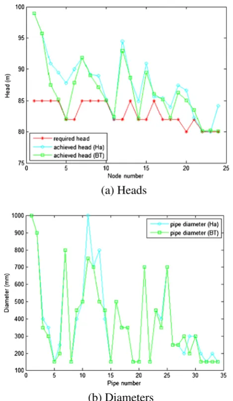
is set to 107 FEs to investigate the performance of the algorithms over a relatively long evolution period. A new least-cost solution of Rs124.69×106is found here using the more restrictive head-loss parameters standard in Epanet 2.0, representing a 5.04 % reduction of the least-cost solution previously reported. The pipe diameters and nodal heads produced by the previous optimal solution of Rs131.31×106and the new optimal solution of Rs124.69×106 are compared in Fig.3. The infeasible head for node 23 for the previous optimal solution is evident in Fig.3(a). In Table1the performance of each algorithm is summarized. It is evident that the MA performs better than the GA in terms of converging to good solutions, achieving a lower average final least-cost solution. Using the HPCUOS with 16 nodes comprising 2 islands the average CPU time for a single optimisation run of 107FEs is 0.943 h for the GA and 0.853 h for the MA. The smallest number of FEs it took to find the optimal solution was 2,572,200 for the GA and 142,000 for the MA.

This network represents a substantial challenge. It has not been widely studied and there are limited details available with regard to the performance of the two algorithms presented for comparison with the MA in Table 2. The termination conditions used here for equitable comparisons are 4,400 FEs and 120,000 FEs. The best costs displayed were found only once by each algorithm and so the rates of converging to these costs are omitted. With the termination condition of 120,000 FEs, the best solution found and the average cost are cheaper for both the MA and the GA than the comparative studies. The best cost found by the GA is within 1 % of the optimal solution given in Table1and the average cost is only 3.6 % greater than this optimal solution. In comparison, the MA locates a solution which is only 0.1 % greater than the optimal solution and on average finds a solution within 1.6 % of the optimal solution. It is evident the performance of the MA is particularly impressive given the relatively small number of FEs allowed.

4.5 Balerma Network

This demonstrates the substantial challenge in designing a real-world WDS. Head-losses are calculated using the Darcy–Weisbach equation with an absolute pipe roughness of k= 0.0025 mm. The required pressure head at each demand node is 20 m. The best solution to date for the Balerma network was found by Zheng et al. (2011) costing M€1.923, with the second best solution found by Tolson et al. (2009) costing M€1.940.

Previous investigations on this network have employed between 10 and 100 random trials over 107FEs, and to the best of our knowledge, no previous investigation has converged to their own best result more than once over all trials. This indicates that these algorithms are not converging over 107FEs. Consequently the GA and the MA are compared here initially using a termination condition of 108FEs in an attempt to achieve better convergence (Table1). The

(a) Heads

(b) Diameters

best solutions found by the GA and MA are M€1.929 and M€1.924 respectively, which are both cheaper than the solution found by Tolson et al. and are both within 0.5 % of the solution found by Zheng et al. The most expensive least-cost solution found was M€1.949 for the GA and M€1.937 for the MA. Each algorithm found its own best solution only once over the 100 random trials; in fact, neither the GA nor the MA converged to the same solution more than once after the 108FEs. This indicates that neither algorithm is converging with respect to the least-cost solution, despite the large number of FEs used. Each run is therefore converging to a similar final population, with the main discernible difference that the least-cost solution is different in each case. From Table1it is clear that the MA outperforms the GA with respect to every measure. In particular, the MA finds a solution within 1 % of the solution found by Zheng et al. in under 4 % of the FEs required by the GA and the final solution found is lower on average with less deviation for the MA than the GA. Using the HPCUOS with 160 processors comprising 20 islands, the average CPU time for a single optimisation run of 108 FEs is 4.919 h for the GA and 4.894 h for the MA.

In Table3the GA and the MA with the termination condition 107FEs are compared with a selection of results from the literature. Using the HPCUOS with 16 processors comprising 16 Table 1 Assessment of the genetic and memetic algorithms

Number of randomly initiated runs 100

Optimization problem a_{Kadu network} b_{Balerma network}

Termination criterion (FEs×106) 10 100

Algorithm GA MA GA MA

Cheapest final cost found (106_{) 124.69 124.69 1.929 1.924} Average final cost found (106_{) 125.48 125.39 1.938 1.928} Standard deviation of final cost (106) 0.313 0.349 0.005 0.003 Average number of FEs required to find a feasible

solution within 1 % of current best (106)

0.6656 0.084 57.80 2.30

Average CPU time per optimization run (hours) 0.943 0.853 4.919 4.894

Costs are ina_{Rupees and}b_{Euros respectively for the}a_{Kadu and}b_{Balerma networks}

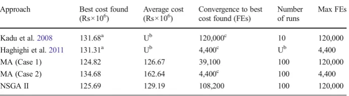
Table 2 Comparison of published results for the Kadu network

Approach Best cost found (Rs×106₎

Average cost (Rs×106₎

Convergence to best cost found (FEs)

Number of runs

Max FEs

Kadu et al.2008 131.68a Ub 120,000c 10 120,000 Haghighi et al.2011 131.31a Ub 4,400c Ub 4,400

MA (Case 1) 124.82 126.67 39,100 100 120,000

MA (Case 2) 134.68 162.64 4,400c _{100 4,400}

NSGA II 125.69 129.19 108,200 100 120,000

a

Hydraulically infeasible solutions b

U indicates this value is unclear from the reference c

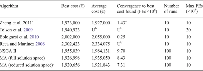
islands the average CPU time for a single optimisation run of 107FEs is 2.18 h for the GA and 1.84 h for the MA. As discussed above, all algorithms in Table3converge to their own best solution only once. The MA performs better than the standard GA with respect to every measure and only the NLP-DE algorithm (Zheng et al.2011) provides better results than the MA. The best cost found by the MA is M€1.927 which is a 0.2 % increase on the best cost found with NLP-DE by Zheng et al. of M€1.923, and the average final cost found by the MA is only 0.4 % greater than that found by NLP-DE. However the NLP-DE algorithm comprises three stages. First the WDS network is converted from a looped network to a branched network by identifying the shortest-distance tree using graph theory. This branched network is then optimised using continuous diameters and a commercial non-linear programming software. The final step uses the non-linear programming solution of the branched network problem to restrict the search space for the initial seeding of a differential evolution optimisation. The differential evolution then proceeds as standard. This approach can therefore be characterised as a differential evolution optimisation with substantial pre-processing of the network. There are no published details regarding the NLP used and any increase in CPU time incurred by the overall NLP-DE procedure compared to the standard DE used in that study. The MA described here is much simpler to implement as it is a purely iterative procedure which is initiated randomly and requires no prior network preparation or analysis. Additionally, the MA is more computationally efficient than the standard GA and requires no external optimiser. The results of Table3indicate that despite the simplicity of the MA, the quality of the solution is comparable with that found by the more complex NLP-DE procedure. Indeed, further improvements were achieved after reducing the solution space as summarized in theAppendix. A new best solution was found.

5 Conclusions

A memetic algorithm (MA) is developed and compared with a robust and widely used genetic algorithm (GA) in the solution of the least-cost water distribution system (WDS) design problem. The problem is formulated as a multi-objective optimisation, with the competing objectives to minimise cost and maximise network performance. Two benchmark WDS networks are used to test the performance of the MA. The MA is found to substantially outperform the GA in each case, demonstrating improved convergence speed and convergence rates. In comparison with other Table 3 Comparison of published results for the Balerma network

Algorithm Best cost (€) Average cost (€)

Convergence to best

cost found (FEs×106₎ Number_{of runs} Max FEs_(×106₎

Zheng et al. 2011a 1,923,000 1,927,000 1.43a 10 10

Tolson et al.2009 1,940,923 Ub Ub 10 30

Bolognesi et al.2010 2,002,000 2,055,000 0.25 10 10 Reca and Martinez2006 2,302,423 2,334,075 Ub 10 10

NSGA II 1,955,039 1,984,131 9.70 100 10

MA (full solution space) 1,926,998 1,935,050 8.43 100 10 MA (reduced solution space)c 1,920,656 1,921,843 7.31 100 10

a

A direct comparison is not obvious as the differential evolution in NLP-DE is preceded by graph theory, NLP and search space reduction

b

U indicates this value is unclear from the reference c

studies in the literature the MA is shown to be highly competitive. This investigation indicates that the local search and cultural improvement operators introduced here could be a useful tool in achieving competitive solutions to the design of real-life WDS networks in tractable time periods. Future investigations could combine the local and cultural improvement operators defined here with alternative baseline GAs, or alternative evolutionary computing techniques.

Acknowledgments This work was supported by the UK Engineering and Physical Sciences Research Council (EPSRC Grant Reference EP/G055564/1).

Appendix: Search Space Reduction on the Balerma Network

For the Balerma network, as an alternative to the protracted optimization runs of 108 FEs in Table 1, we used engineering judgement to reduce the search space prior to the optimisation. The number of decision variables was reduced from 454 to 171 by removing the decision variables whose optimal values did not vary across the previ-ous investigations. The remaining 171 decision variables were then restricted to three possible pipe sizes based on the previous investigations. This process reduced the search space from 10454 to 3171 or 3.87 ×1081 possible solutions. Applying the MA to this reduced problem yielded a new optimal solution after 107 FEs of €1,920,656, which was found once out of 100 random runs. Details on the 100 runs of the MA on this reduced problem are also included in Table 3. The median, maximum and the standard deviation of the least-cost solutions found across the 100 runs are

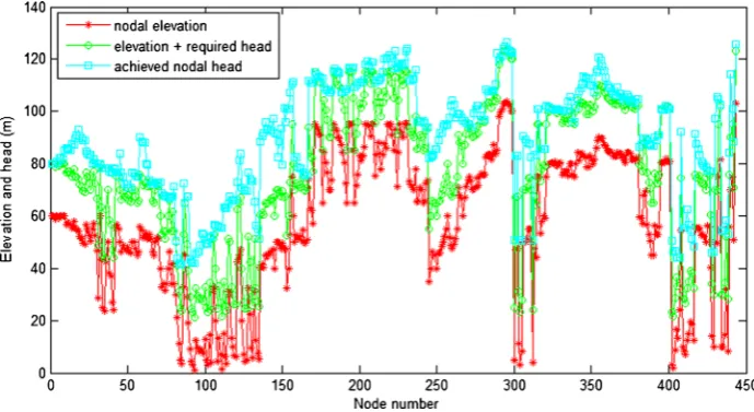
€1,921,708,€1,923,897 and€707 (0.04 % of the corresponding mean value in Table3) respectively. These solutions are a substantial improvement on any other method in Table 3. Using the HPCUOS with 16 processors comprising 16 islands the average CPU time for a single optimisation run of 107 FEs is 1.97 h. The nodal heads for the new best solution (€1,920,656) are given in Fig. 4. The pipe diameters can be found in Online Resource 1.

Open AccessThis article is distributed under the terms of the Creative Commons Attribution License which permits any use, distribution, and reproduction in any medium, provided the original author(s) and the source are credited.

References

Banos R, Gil C, Reca J, Martinez J (2009) Implementation of scatter search for multi-objective optimization: a comparative study. Comput Optim Appl 42:421–441

Banos R, Gil C, Reca J, Montoya FG (2010) A memetic algorithm applied to the design of water distribution networks. Appl Soft Comput 10:261–266

Berendsen HJC (2011) A student’s guide to data and error analysis. Cambridge University Press, Cambridge Bolognesi A, Bragalli C, Marchi A, Artina S (2010) Genetic heritage evolution by stochastic transmission in the

optimal design of water distribution netwroks. Adv Eng Soft 41:792–801

Cisty M (2010) Hybrid genetic algorithm and linear programming method for least-cost design of water distribution systems. Water Resour Manag 24:1–24

Deb K, Pratap A, Agarwal S, Meyarivan T (2002) A fast and elitist multi-objective genetic algorithm: NSGA-II. IEEE Trans Evol Comp 6(2):182–197

di Pierro F, Khu ST, Savic D, Berardi L (2009) Efficient multi-objective optimal design of water distribution networks on a budget of simulations using hybrid algorithms. Environ Model Softw 24:202–213 Erfani T, Utyuzhnikov S (2011) Directed search domain: a method for even generation of the Pareto frontier in

multiobjective optimization. Eng Optimiz 43(5):467–484

Eusuff MM, Lansey KE (2003) Optimization of water distribution network design using the shuffled frog leaping algorithm. J Water Res Pl-ASCE 129(3):210–225

Guo Y, Keedwell EC, Walters GA, Khu ST (2007) Hybridizing cellular automata principles and NSGA II for multi-objective design of urban water networks. EMO 2007:546–549

Haghighi A, Samani HMV, Samani ZMV (2011) GA-ILP method for optimization of water distribution networks. Water Resour Manag 25(7):1791–1808

Kadu MS, Gupta R, Bhave R (2008) Optimal design of water networks using a modified genetic algorithm with reduction in search space. J Water Res Pl-ASCE 134(2):147–160

Kanakoudis VK (2004) Vulnerability based management of water resources systems. J Hydroinformatics 6(2): 133–156

Miettinen KM (1998) Nonlinear multiobjective optimization. Kluwer Academic Publishers, Boston

Reca J, Martinez J (2006) Genetic algorithms for the design of looped irrigation water distribution networks. Water Resour Res 42, W05416

Rossman LA (2000) Epanet 2 user’s manual. US Environmental Protection Agency, Cincinnati

Siew C, Tanyimboh TT (2012) Penalty-free feasibility boundary convergent multi-objective evolutionary algorithm for the optimization of water distribution systems. Water Resour Manag 26(15):4485–4507. doi:

10.1007/s11269-012-0158-2

Skipworth P, Engelhardt M, Cashman A, Savic D, Daul A, Walters G (2002) Whole life costing for water distribution network management. Thomas Telford Publishing, London

Tanyimboh TT, Kalungi P (2008) Optimal long-term design, rehabilitation and upgrading of water distribution networks. Eng Optimiz 40(7):637–654

Tanyimboh TT, Kalungi P (2009) Multicriteria assessment of optimal design, rehabilitation and upgrading schemes for water distribution networks. Civ Eng Environ Syst 26(2):117–140

Tolson BA, Asadzadeh M, Maier HR, Zecchin A (2009) Hybrid discrete dynamically dimensioned search (HD-DDS) algorithm for water distribution system design optimization. Water Resour Res 45, W12416 Zheng F, Simpson AR, Zecchin A (2011) A combined NLP-differential evolution algorithm approach for the