Estimating the Expected Value of Sample
Information Using the Probabilistic
Sensitivity Analysis Sample: A Fast,
Nonparametric Regression-Based Method
Mark Strong, PhD, Jeremy E. Oakley, PhD, Alan Brennan, PhD, Penny Breeze, PhD
Health economic decision-analytic models are used to estimate the expected net benefits of competing decision options. The true values of the input parameters of such models are rarely known with certainty, and it is often use-ful to quantify the value to the decision maker of reducing uncertainty through collecting new data. In the context of a particular decision problem, the value of a proposed research design can be quantified by its expected value of sample information (EVSI). EVSI is commonly esti-mated via a 2-level Monte Carlo procedure in which plau-sible data sets are generated in an outer loop, and then, conditional on these, the parameters of the decision model are updated via Bayes rule and sampled in an inner loop. At each iteration of the inner loop, the decision model is evaluated. This is computationally demanding and may be difficult if the posterior distribution of the model pa-rameters conditional on sampled data is hard to sample
from. We describe a fast nonparametric regression-based method for estimating per-patient EVSI that requires only the probabilistic sensitivity analysis sample (i.e., the set of samples drawn from the joint distribution of the parameters and the corresponding net benefits). The method avoids the need to sample from the posterior dis-tributions of the parameters and avoids the need to rerun the model. The only requirement is that sample data sets can be generated. The method is applicable with a model of any complexity and with any specification of model parameter distribution. We demonstrate in a case study the superior efficiency of the regression method over the 2-level Monte Carlo method. Key words: expected value of sample information; economic evaluation model; Monte Carlo methods; Bayesian decision theory; computational methods; nonparametric regression; generalized additive model.(Med Decis Making 2015;35:570–583)
H
ealth economic decision-analytic models are used to estimate the expected net benefits of competing decision options. The true values of theinput parameters of such models are rarely known with certainty, and uncertainty in model parameters typically results in decision uncertainty. This may motivate decision makers to consider options for further data collection alongside the adoption of new technologies or to delay adoption until after data collection.1,2 The value of learning an input parameter (or a group of input parameters) can be quantified by its partial expected value of perfect information (partial EVPI).3–6 However, we are unlikely to be able to collect perfect information, Received 17 June 2014 from the School of Health and Related
Research (ScHARR), University of Sheffield, Sheffield, UK (MS, AB, PB), and School of Mathematics and Statistics, University of Sheffield, Sheffield, UK (JEO). Mark Strong is funded by a postdoctoral fellowship grant from the National Institute for Health Research (PDF-2012-05-258). The funding agreement ensured the authors’ independence in designing the study, interpreting the data, writing, and publishing the report. This report is independent research supported by the National Institute for Health Research (PDF-2012-05-258). The views expressed in this publication are those of the author(s) and not necessarily those of the NHS, the National Institute for Health Research, or the Department of Health. Revision accepted for publication 9 January 2015.
ÓThe Author(s) 2015 Reprints and permission:
http://www.sagepub.com/journalsPermissions.nav DOI: 10.1177/0272989X15575286
Supplementary material for this article is available on the Medical Decision MakingWeb site at http://mdm.sagepub.com/supplemental.
and it is more useful to quantify the value of specific research designs that will inform the decision-making problem. The value ofreducing, rather than
eliminating, uncertainty through the collection of data is captured by the expected value of sample information (EVSI).4,7,8
The EVSI for any particular data collection exer-cise will depend not only on the study design in ques-tion but also on the decision context.8 Important factors include whether there are costs associated with either delaying or reversing adoption deci-sions,1,9,10 whether the adoption decision will be fully implemented11and whether the proposed study extends across jurisdictions.12,13Some of these fac-tors arise in moving from EVSI per patient to popula-tion EVSI, but others also arise in estimating EVSI per patient. While recognizing these issues, we do not discuss them further in this article but concentrate on the problem of computing per-person EVSI within a single jurisdiction under the assumption of costless reversibility with perfect implementation and with no delay in either the study or the adoption.
The concept of EVSI was first discussed in the health economics literature well over a decade
ago.4,7,14,15 Despite this, very few research funding
or design decisions are informed by EVSI. This, at least in part, reflects the computational burden of cal-culating EVSI via generic Monte Carlo sampling-based methods. For example, in a recently published cost-effectiveness study, the authors noted that to compute EVSI without assuming an approximation that the model was linear, it would have taken 7.5 days.16In another example, the proposed EVSI anal-ysis would have taken 37.5 days.17Clearly, computa-tion times of this order are prohibitive.
The reason for the high computational cost of EVSI analysis is that, unless the model is of a certain form or unless certain parametric assumptions are made, a nested 2-level Monte Carlo scheme is required. In this scheme, plausible data sets are generated in an outer loop, and then conditional on each data set, samples are generated from the posterior distribution of the parameters in an inner loop. The model is run with each inner loop set of parameters to estimate the expected net benefits, conditional on the data sets that have been simulated in the outer loop. The computational cost arises primarily due to the repeated evaluation of the model within the inner loop but also due to the burden of repeated sampling in the inner loop. If the aim is to search over the study design space, then this problem is further com-pounded because EVSI itself must be repeatedly cal-culated. Another difficult arises with the 2-level
Monte Carlo approach if the prior distribution of the model parameters is not conjugate to the data likeli-hood. In this case, generating the inner-loop samples will typically require Markov chain Monte Carlo (MCMC), and the repeated application of MCMC for each sampled data set adds to the computational burden.
A fast approximation scheme for the inner-loop step has been proposed,18,19but this method requires repeated evaluation of partial derivatives of the log posterior density function and therefore considerable time and effort writing the necessary computer code on the part of the analyst. Computationally cheaper single-loop approaches are sometimes available, but these rely either on the model being of a certain
form7,20,21 or on assumptions of Normality of the
mean incremental net benefits.1 Fast single-loop
methods also exist for computing partial EVPI for sin-gle parameters,22,23 but these have not yet been extended to the computation of EVSI.
In this article, we present a method for calculating per-patient EVSI that avoids the nested 2-level scheme, requiring only the single set of sampled model inputs and corresponding model outputs (i.e., net benefits) that is generated in a standard prob-ability sensitivity analysis (PSA). The method is based on a nonparametric regression of the net ben-efits on data samples that are generated conditional on the sampled input parameters in the PSA and fol-lows closely the nonparametric regression method for computing partial EVPI described in Strong et al.24The method makes no assumptions regarding the form of the model, does not require the use of MCMC, and does not require that the parameter prior is conjugate to the data likelihood. All that is required is that the data likelihood can be sampled (but not necessarily evaluated). The article is structured as follows. In the second section, we introduce the method and describe its general appli-cation. In the third section, we demonstrate the method in the case study model that was used for illustrative purposes in Ades et al.,7 and in the fourth section, we present results. We conclude with a short discussion.
METHOD
We assume that we are faced with D decision options, indexedd= 1, . . .,D, and have built a model NB(d,u) that aims to predict the net benefit of deci-sion optiondgiven a vector ofpinput parameter val-ues u = (u1, . . ., up). The true values of the input
parameters are assumed to be unknown, and we rep-resent beliefs about the input parameters via their joint distribution p(u). We index a sample drawn from the joint distribution of the parameters with a bracketed superscript, u(n), for sample draws n = 1, . . .,N.
We envisage that we can collect data that will be informative for some subset of parameters. We con-sider the (as yet uncollected) data as a vector of ran-dom variables and denote this as uppercase X. We use lowercasexfor some arbitrary realized (or sam-pled) vector of values from the distribution ofX. We use the bracketed superscript notation to index a sam-ple of data vectorsx(n),n= 1, . . .,N.
We denote the expectation over the joint distribu-tion ofu asEu. We denote the expectation over the
distribution of the dataXasEXand over the posterior
distribution ofugiven dataXasEujX.
The expected value of our optimal decision, made only with current information is
max
d EufNBðd;uÞg: ð1Þ
If we had dataXthat were informative for (some sub-set of) the inputs, then the optimal decision would be that with the greatest net benefit, after averaging over the joint distribution of the inputs conditional on the data,p(u|X). The expected net benefit would be
max
d EujXfNBðd;uÞg: ð2Þ
But, since X is uncollected, we must average over possible data sets,
EX max
d EujXfNBðd;uÞg
: ð3Þ
The distribution ofXcan be obtained by the margin-alization of p(X, u) = p(X|u)p(u), which suggests a straightforward Monte Carlo sampling scheme for X, that is, sample first a valueu*from the priorp(u) and then sampleXfrom the data likelihoodp(X|u= u*). Note that the data likelihood will depend on the design of the study under consideration, and we return to this point when we discuss our case study. The EVSI is then the difference between equation (3) and equation (1),
EVSI5EX max
d EujXfNBðd;uÞg
max
d EufNBðd;uÞg: ð4Þ
At this point, we note that we can reexpress (4) as
EVSI5EX max
d EujXfNBðd;uÞg
max
d EX EujXfNBðd;uÞg
:
ð5Þ
The reason for the reexpression will become appar-ent when we discuss Monte Carlo sampling schemes for estimating EVSI.
The Monte Carlo Approach to Computing EVSI
A probabilistic sensitivity analysis (PSA) takesN
samples from the joint distribution of the input parameters, {u(1), . . ., u(N)}, and generates a corre-sponding set of N net benefits {NB(d, u(1)), . . ., NB(d, u(N))} for each decision option d. From this, the usual Monte Carlo solution to the second term in equation (4) is
max
d EufNBðd;uÞg ’maxd
1
N
XN
n51
NBðd;uðnÞÞ: ð6Þ
The first term in equation (4) requires more work, and unless there are analytic solutions to the expecta-tions, the usual approach is to use a nested 2-level Monte Carlo method.7Here, the estimator is given by
EX max
d EujXfNBðd;uÞg
’ 1
K
XK
k51
max
d
1
J
XJ
j51
NBðd;uðj;kÞÞ;
ð7Þ
whereu(j,k)are samples drawn from the posterior dis-tribution ofu|x(k), andx(k)are generated by first sam-plingu(k)fromp(u) and thenx(k)fromp(X|u=u(k)). Subtracting equation (6) from equation (7) results in the 2-level Monte Carlo EVSI estimator
d
EVSI51
K
XK
k51 max
d
1
J
XJ
j51
NBðd;uðj;kÞÞ max
d
1
N
XN
n51
NBðd;uðnÞÞ:
ð8Þ
However, if we arrange our sampling scheme such that it reflects equation (5), we obtain instead
d
EVSI51 K
XK
k51
max d
1
J XJ
j51
NBðd;uðj;kÞÞ max d
1
K XK
k51
1
J XJ
j51
NBðd;uðj;kÞÞ
Here, both terms in the EVSI expression are evaluated using the same sampled values of u, and hence we will obtain an estimator with smaller Monte Carlo error than if we were to use equation (8).
The first problem with the nested 2-level scheme is the requirement to evaluate the net benefit function (i.e., to run the model) at each iteration of the inner loop, resulting in J 3 K model evaluations. If the model is slow to run and/or ifJ andKare large (to obtain adequate precision), then the scheme will be computationally burdensome. A second potential problem is the requirement to sample from the poste-rior distribution of the input parameters, conditional on the sampled data, that is, obtaining thej= 1, . . .,J
samplesu(j,k)from eachp(u|x(k)) in the inner loop. If
p(X|u) andp(u) are conjugate, then the posterior dis-tribution will be of a known form, and sampling from it will be straightforward. However, if conjugate forms are not appropriate, we may be required to resort to MCMC to generate thej= 1, . . .,Jsamples u(j,k)fromp(u|x(k)). The MCMC step must be repeated for each of thek= 1, . . .,Ksampled data values, and this will add considerably to the computational bur-den. Setting up the MCMC sampler (e.g., via writing BUGS code25) and checking the MCMC chain(s) for convergence also requires investment in modeler time.
We note at this point that in some restricted cases, we can avoid entirely the inner-loop Monte Carlo step. If the model is linear or multilinear (i.e., of ‘‘sum-product’’ form) in the parameters, and if the parameters are independent of one another (and retain this independence after updating with data), and if we can analytically compute the posterior expectations of the parameters given the data, then we can simply ‘‘plug in’’ the expected parameter val-ues into the net benefit equation to obtain the expected net benefit.7,21,26
Nonparametric Regression Method
The problem with the 2-level Monte Carlo scheme is the need to compute the inner expectation in the first term in equation (4) via Monte Carlo. Not only does this require Jmodel runs for each outer loop, but it is this step that requires the potentially prob-lematic sampling from the conditional distribution
p(u|X). We therefore propose to estimate this expec-tation as follows.
Consider generating a random parameter vectoru from p(u) and a random data sample Xconditional on u and then evaluating NB(d, u). We recognize that we can express the observed NB(d, u) as a sum
of the conditional expectation that we require and a mean-zero error term,
NBðd;uÞ5EujXfNBðd;uÞg1e; ð10Þ
where the erroreis a function of bothXandu. To see whyehas zero mean, we rearrange to give
e5NBðd;uÞ EujXfNBðd;uÞg; ð11Þ
and then take expectations with respect to bothXand u, giving
EX;uðeÞ5EX;ufNBðd;uÞg EX;u½EujxfNBðd;uÞg 5EufNBðd;uÞg EX½EujxfNBðd;uÞg;
noticing that the first term in the right-hand side of equation (11) is a function only ofuand the second term a function only of X(uhaving been integrated out). Then, by the law of total expectation (or ‘‘tower rule’’),EX½EujxfNBðd;uÞg5EfNBðd;uÞg, and hence EðeÞ50. Note that this holds regardless of the distri-bution ofuand regardless of the relationship between uandX.
Next, we recognize that the expectation EujXfNBðd;uÞgcan be thought of as an unknown func-tion of X. We denote this function g(d, X), and substituting this into equation (10) gives
NBðd;uÞ5gðd;XÞ1e: ð12Þ
In some instances, the data X will be high dimen-sional (e.g., censored time-to-event data in a study that measures survival), and if this is so, we write the function g in terms of some low-dimensional summary statistic of the data T(X) = {T1(X), . . .,
Tp(X)}, giving
NBðd;uÞ5gfd;TðXÞg1e: ð13Þ
We discuss choice of summary statistic in the next section.
GAM models assume that the expectation of the dependent variable is a smooth but usually unknown function of the independent variable, which is exactly what we need here. The standard linear model is a special case of the GAM model in which the functional form of the expectation of the depen-dent variable is specified a priori.
When we adopt a GAM model, we usually repre-sent the unknown underlying smooth function as some form ofspline, a common choice being thecubic spline. In the simplest case, a univariate cubic spline represents an arbitrary smooth single-input function as a series of short cubic polynomials joined piece-wise such that the function is twice-differentiable at the ‘‘knots’’ (i.e., join points). The same spline can also be represented as the weighted sum of a series of predetermined ‘‘basis functions’’ that extend over the whole range of the function input. Simple univar-iate cubic splines have natural extensions to higher dimensions and to a regression framework, where the spline parameters (i.e., the basis function weights) are estimated from noisy data. For an introduction to GAM models, see Hastie and Tibshirani27or Wood.28 Returning now to the problem of estimating g{d, T(X)}, we obtain the necessary ‘‘data’’ for the GAM regression analysis as follows. We assume we have at our disposal a PSA sample of sizeK. This consists of a set ofk= 1, . . .,Ksamples from the distribution of the input parametersu(k), andk= 1, . . .,K correspond-ing evaluations of the model NB(d,u(k)), for each deci-sion optiond= 1, . . .,D. The dependent variable for regressiondis the net benefit NB(d,u(k)) for decision optiond. To generate realizations of the independent variable (which is common to alld= 1, . . .,D regres-sion analyses), we sample, for each valueu(k), a data set x(k)from the likelihood p(X|u =u(k)) and, from x(k), calculate the summary statistic T(x(k)). At no point do we attempt to derive or sample from the potentially difficult posterior distribution of the parameters, p(u|x(k)), and at no point do we rerun the economic model. This is why the method is fast and simple.
We note here that EVSI is invariant to the reexpres-sion of net benefits as incremental net benefits, rela-tive to some chosen ‘‘baseline’’ option. Under this reexpression, the (incremental) net benefit of the baseline option is zero. This reduces the number of regression equations fromDtoD21.
Choice of Summary StatisticT()
Study data xmay be scalar or vector valued and may be informative for one or more economic model
parameters. In the simplest case, we have scalar data that are informative for a single economic model parameter. Here we chooseT(x) =x. Ifxis vector val-ued, but we still expect data only to update a single model parameter ui, and then we choose T(x) to be
a sample estimator forui. This leads to quite natural summary statistics. So, for example, if we wish to cal-culate the expected value of a 2-arm, binary outcome trial to update beliefs about an odds ratio, then we our choice ofT(x) would be the sample odds ratio.
If we wish to update beliefs aboutq.1 economic model parameters {u1, . . .,uq}, then we would calcu-late q summary statisticsT(x) = {T1(x), . . ., Tq(x)},
where each Ti(x) is a sample estimator for ui. For
example, if we wish to calculate the expected value of a study to learn about the shape and scale parame-ters of a Weibull distribution, {u1,u2}, andxare cen-sored time-to-event data, then we would choose {T1(x), T2(x)} to be the sample estimates fu^1;^u2g
derived from a Weibull survival model.
In the case ofq. 1, we write the vector of scalar summary statistics asT(x) = {T1(x), . . .,Tq(x)}, and
fit the GAM model NB (d,u) =g{d, T(x)} +e, where
gis now a multivariate smoothing function.28 Hypothetical Nonparametric Regression Example
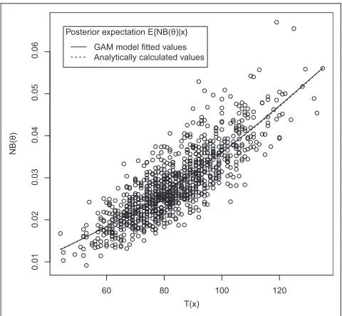
To give an example, we imagine a hypothetical net benefit function NB(u) =u2(for clarity, we have drop-ped the decision option indexdin this example). The parameterurepresents a proportion (e.g., of people in the population who have a certain characteristic), and current knowledge about the proportion is expressed via a Beta(40,200) distribution. We want to know the value of doing a study with 500 partici-pants to learn about the proportion. The number of people in the study with the characteristic of interest, x, is modeled using a Binomial(u, 500) distribution.
The PSA sample comprises samples {u(1), . . .,u(K)} with the corresponding samples from the net benefit function {NB(u(1)), . . ., NB(u(K))}. For each sampleu(k), we generate a sample of datax(k)fromX|u(k)~ Bino-mial (u(k), 500). The data here are scalar, and we there-fore chooseT(x) =x. We fit a GAM regression of NB(u) on T(x) and extract the fitted values, which are our estimates ofEujxfNBðuÞg. In this hypothetical exam-ple, we can calculate EujxfNBðuÞg analytically, so can compare the GAM regression values with their true counterparts.
sampled values of T(x). The solid line shows the GAM model fitted values, and the dashed line shows the analytically calculated values.
Regression Diagnostics
As with all regression analysis, it is important to check assumptions. Most important, we require that there is no structure in the residuals (e.g., a U-shaped or S-shaped pattern) since this would suggest unmodeled structure in the target function g and therefore bias in the fitted values. We note that for the purposes of calculating EVSI, we are seeking to estimate only the posterior mean net benefits. We do not require the posterior variance of the net bene-fits for the EVSI computation and therefore whether the residuals have equal variance and follow a partic-ular distribution is of secondary importance.29
In contrast to the estimator for the EVSI, the esti-mator for the Monte Carlo standard error of the EVSI given in the online Appendixdoesrely on the net benefits having approximately equal variance and approximate Normality if the number of rows of the PSA is small. However, if the size of the PSA is large, then the standard error estimator can be justi-fied on large sample results, even in the absence of Normality of the net benefits (see Appendix).28
EVSI Calculation
After fitting a GAM model for each decision option
d, we then extract the regression model fitted values. The fitted values are estimates of g{d, T(x(k))}, k = 1, . . .,K, our target quantity. We denote the GAM fit-ted values for decision optiondasg^ðdkÞ, and the esti-mated EVSI is then given by
d
EVSI5 1 N
XN
k51
max
d g^
ðkÞ
d maxd
1
K
XK
k51
^
gdðkÞ: ð14Þ
Note that we choosemaxdK1 PK
k51g^
ðkÞ
d rather than
maxdK1 PK
K51NBðd;uðkÞÞ as the second term in the
EVSI estimator, following expression (5) rather than expression (4). By choosing this as our estimator, we exploit the positive correlation between the two terms in equation (14) and hence estimate the EVSI with increased precision.
The sampling scheme for the GAM regression-based EVSI is given in Box 1.
Because we are averaging overk, we can think of this as a single-loop Monte Carlo method. The size of Kwill determine the precision of the estimate of the EVSI, and a method for estimating the standard error of the GAM-based approximation is given in the Appendix.
60 80 100 120
0.01
0.02
0.03
0.04
0.05
0.06
T(x)
NB(
θ
)
[image:6.594.48.288.92.314.2]Posterior expectation E{NB(θ)|x} GAM model fitted values Analytically calculated values
Figure 1 Hypothetical example. Generalized additive model (GAM) model fitted values of the posterior expected incremental net benefit versus analytic values. The lines representing the GAM fitted and analytic values are almost indistinguishable.
Box 1 Generalized Additive Model (GAM) Regres-sion-Based EVSI Algorithm
Generate a PSA sample of size K:
fork= 1, . . .,Kdo
Sampleu(k)from the distribution of the parameters,
p(u)
Evaluate the economic model to obtain (incremental)
net benefits NB(d,u(k))
end for
Given the PSA sample, simulate data samples:
fork= 1, . . .,Kdo
Generate a data samplex(k)fromp(X|u(k))
Calculate summary statisticT(x(k))
end for
Fit regression models and calculate EVSI:
Regress net benefits NB(d,u(k)) from the PSA onT(x(k))
for eachd
Extract GAM model fitted values for eachd
Calculate EVSI via equation (14).
CASE STUDY: ADES (2004) DECISION TREE MODEL
Model
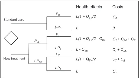
Our case study is based on the model that was used for illustrative purposes in Ades et al.7The decision problem has two options:d = 1 (standard care) and
d= 2 (new treatment) and can be represented by a sim-ple decision tree (Figure 2). There are 11 parameters in the model, which we write as the vector u = (L, QE, QSE, CE, CT, CSE, PC, PSE, OR, PT,l). Parameter
def-initions and distributions are given in Table 1. The output of the model is the net benefit for each deci-sion option in monetary units. The algebraic form of the model is given in equations (15) and (16), with some components ofubeing redundant in each net benefit function.
NBð1;uÞ5PCflLð11QEÞ=2CEg1ð1PCÞlL: ð15Þ
NBð2;uÞ5PSEPT½lfLð11QEÞ=2QSEg ðCT1CSE1CEÞ1 PSEð1PTÞ flðLQSEÞ ðCT1CSEÞg1
ð1PSEÞPTflLð11QEÞ=2 ðCT1CEÞg1
ð1PSEÞ ð1PTÞ ðlLCTÞ: ð16Þ
The model is multilinear in the parameters, and all parameters are independent. Thus, the expectation of the net benefit,EfNBðd;uÞg, is equal to the net ben-efit equation evaluated at the parameter expectations, NBfd;EðuÞg. This is generally the case for decision tree models with independent parameters but not for Markov models or individual-level simulation models.
For our case study, we consider the same 3 data collection scenarios presented in Ades et al.7—that is, data collection to inform the probability of side effects (PSE), the quality of life after critical event
(QE), and the treatment effect size (OR). For each
[image:7.594.48.546.107.249.2]sce-nario, we calculated EVSI using 3 methods. First, we replicated the method presented in Ades et al. The method relies on the model being of multilinear form with independent parameters and that there are analytic solutions (or good approximations) to the posterior expectations of the parameters, condi-tional on simulated data. Hence, the method only requires a single-loop Monte Carlo scheme to evalu-ate the outer expectation in the first term in equation (4). Second, we used the 2-level Monte Carlo scheme outlined earlier, with an MCMC inner loop. This method does not rely on the model being multilinear with independent parameters or that there are ana-lytic solutions to the posterior expectations of the parameters. However, it has high computational cost. Third, we used the GAM regression method pre-sented earlier. As with the Ades et al. method, the Table 1 Case Study Parameter Distributions
Description Parameter Mean Distribution
Mean remaining lifetime L 30 Constant
QALY after critical event, per year QE 0.6405 logit(QE);N(0.6, 1/6)
QALY decrement due to side effects QSE 1 Constant
Cost of critical event CE $200,000 Constant
Cost of treatment CT $15,000 Constant
Cost of treatment side effects CSE $100,000 Constant
Probability of critical event, no treatment PC 0.15 Beta(15,85)
Probability of treatment side effects PSE 0.25 Beta(3,9)
Odds ratio, (PT/(12PT))/(PC/ (12PC)) OR 0.2636 log(OR);N(–1.5, 1/3)
Probability of critical event on treatment PT 0.0440 [derived fromORandPC]
Monetary value of 1 QALY l $75,000 Constant
QALY, quality-adjusted life year. Adapted from Ades et al.7CopyrightÓ2004. Reprinted with permission from SAGE Publications.
Standard care
New treatment
1-PC
PC
1-PT
1-PT
PT
PT
PSE
1-PSE
Health effects Costs
L L(1 + QE)/2
L(1 + QE)/2 - QSE
L - QSE
L L(1 + QE)/2
CT CT+ CE CT+ CSE CT+ CSE+ CE 0
CE
[image:7.594.48.288.283.418.2]GAM method uses Monte Carlo to evaluate the outer expectation in the first term in equation (4). For con-sistency, we use K to denote the size of the outer expectation Monte Carlo loop when reporting all 3 methods.
Because all 3 methods use Monte Carlo to estimate the outer expectation in equation (4), there will be a Monte Carlo sampling error that tends to zero as the outer-loop sampling size increases. For each esti-mated EVSI, we calculated the Monte Carlo standard error using the methods presented in the Appendix. We repeated each analysis with a range of values of
K to demonstrate the relationship between K and the Monte Carlo standard error. We also recorded the total CPU time required to undertake the EVSI computation to compare the efficiency of each method at different values ofK.
For the Ades et al.7method, we chose values ofK
equal to 104, 105, and 106. For the MCMC-based method, we chose an inner-loop sample size of J= 104after an initial exploration to determine an ade-quate sample size to achieve stability of the inner-loop estimates. We then chose values ofKequal to 104, 105, and 106. Values of K greater than this required prohibitively long runtimes. For the GAM-based method, we chose values of K equal to 104, 105, and 106.
Data Collection Scenario 1: EVSI for the Probability of Side Effects (PSE)
To reduce uncertainty about PSE, we considered
the value of undertaking an observational study of
n = 60 patients on the new treatment. The number of participants observed to experience a side effect is assumed to follow a Binomial(PSE, 60) distribution.
Method 1—single-loop method presented in Ades et al.
In method 1, we replicated the single-loop method used in the case study in Ades et al.7First, we drewk= 1, . . .,Ksamples from the Beta(3, 9) prior distribution forPSE. Next, for each sampled valueP
ðkÞ
SE, we
gener-ated a sample of datax(k)from a Binomial(PðkÞ
SE, 60)
dis-tribution. Due to conjugacy, the posterior distribution has the closed formPSE|x(k)~ Beta (3 +x(k), 692x(k)),
with expectation EPSEjxðkÞðPSEÞ5ð31xðkÞÞ=72.
Because the economic model is multilinear in the parameters, we can calculate for each data setk the exact expected net benefit EujxðkÞfNBðd;uÞg by
plug-ging into equations (15) and (16) the posterior expecta-tionEPSEjxðkÞðPSEÞ, along with the expected values for
the remaining uncertain parameters, EðQEÞ, EðPCÞ, andEðPTÞ. Finally, we estimated the EVSI by
d
EVSI5 1 K
XK
k51
max
d EujxðkÞfNBðd;uÞg
max
d
1
K
XK
k51
EujxðkÞfNBðd;uÞg
h i
: ð17Þ
Method 2—2-level nested Monte Carlo/MCMC sampling scheme
In method 2, we implemented the generic 2-level Monte Carlo scheme outlined earlier. In an outer loop, we drewk= 1, . . .,Ksamples from the Beta(3, 9) prior distribution forPSE. For each valuePðSEkÞ, we
generated a sample of datax(k)from a Binomial(PðSEkÞ, 60) distribution. Conditional on each simulated trial data valuex(k), we then ran an inner-loop of sizeJ= 104. At each run of the inner loop, we sampled a vec-tor of parameter valuesu(j,k)from the posterior distri-butionp(u|x(k)) and evaluated the model net benefit equation NB(d, u(j,k)). Finally, we calculated EVSI via equation (9). Becausex(k)is only informative for the parameterPSE, andPSEis independent of all other
model parameters, drawing fromp(u|x(k)) reduced in this case to drawing from the posterior distribution
p(PSE|x(k)) and the prior distributions for the
remain-ing parameters. Although the posterior distribution
p(PSE|x(k)) has a known form in this example, we
did not assume that this was so and implemented the inner loop in OpenBUGS.25 At each inner-loop step, we discarded the first 1000 MCMC samples as a burn-in.
Method 3—GAM regression
In method 3, we implemented the GAM regression scheme outlined earlier. First, we generated a PSA sample of sizeK. We calculated the incremental net benefit for each PSA sample. Next, for each parameter vectoru(k)in the PSA sample, we generated a sample of data x(k) from a Binomial(PðSEkÞ, 60) distribution. Because the data in this case are scalar, the summary statistic isT(x(k)) =x(k). We regressed the incremental net benefits onT(x(k)), extracted the model-fitted val-ues, and estimated the EVSI via equation (14).
Data Collection Scenario 2: EVSI for Quality of Life after Critical Event (QE)
To reduce uncertainty aboutQE, we considered the
100 patients who have experienced a critical event. We assume that, conditional on QE, the sample
mean of the logit transform of the quality of life reported in a single data collection exercise is Nor-mally distributed with expectation logit(QE) and
var-iance s2/n, where s2, the population variance, is assumed known and equal to 2 (see Ades et al.7for details).
Method 1—single-loop method presented in Ades et al.
As in scenario 1, we replicated the single-loop method used in the case study in Ades et al.7 First, we drewk= 1, . . .,Ksamples from the Normal(0.6, 1/6) prior distribution for logit(QE). Next, for each
sampled value logit(QE)(k), we generated a sample
of datax(k)from a Normal{logit(QE)(k), 1/50}
distribu-tion. Due to conjugacy, the posterior distribution of logit(QE)|x(k) is Normal{(0.6 3 6 + x(k) 3 50)/
(50 + 6),1/(50 + 6)}. The posterior expectation EQEjxðkÞðQEÞcan then be estimated from the posterior distribution of the logit-transformed parameter,
p(logit(QE)|x(k)), using a Taylor series method
(described in full in Ades et al.). Because the eco-nomic model is multilinear in the parameters, we can calculate for each data setkthe expected net ben-efitsEujxðkÞfNBðd;uÞgby plugging into equations (15)
and (16) the posterior expectationEQEjxðkÞðQEÞ, along
with the expected values for the remaining uncertain parameters,EðPSEÞ,EðPCÞandEðPTÞ. We estimated EVSI as described for scenario 1 using equation (17).
Method 2—2-level nested Monte Carlo/MCMC sampling scheme
In method 2, we implemented the 2-level Monte Carlo scheme outlined earlier. In an outer loop, we drewKsamples from the Normal(0.6, 1/6) prior dis-tribution for logit(QE). For each value logit(QE)(k),
we generated a sample of datax(k)from a Normal{lo-git(QE)(k), 1/50} distribution. Conditional on each
simulated trial data valuex(k), we then ran an inner loop of sizeJ = 104. At each run of the inner loop, we sampled a vector of parameter valuesu(j,k)from the posterior distribution p(u|x(k)) and evaluated
the model net benefit equation NB(d,u(j,k)). Finally, we calculated EVSI via equation (9). Becausex(k)is only informative for the parameterQE, andQEis
inde-pendent of all other model parameters, drawing from
p(u|x(k)) reduced in this case to drawing from the posterior distributionp(QE|x(k)) and the prior
distri-butions for the remaining parameters. The posterior distribution p(QE|x(k)) does not have a standard
form, and we therefore implemented the inner loop in OpenBUGS.25 At each inner-loop step, we dis-carded the first 1000 MCMC samples as a burn-in.
Method 3—GAM regression
In method 3, we implemented the GAM regression scheme outlined earlier. First, we generated a PSA sample of sizeK. We calculated the incremental net benefit for each PSA sample. Next, for each parameter vectoru(k)in the PSA sample, we generated a sample of datax(k)from a Normal{logit(QE)(k), 1/50}
distribu-tion. Because the data are scalar, the summary statis-tic isT(x(k)) =x(k). We regressed the incremental net benefits onT(x(k)), extracted the model-fitted values, and estimated the EVSI via equation (14).
Data Collection Scenario 3: EVSI for the Treatment Effect Size (OR)
To reduce uncertainty about the treatment effect size parameterOR, we consider the value of undertak-ing a randomized controlled trial withn= 200 patients allocated to the new treatment, andn= 200 patients allocated to standard care. We assume that, condi-tional on PC and PT, where logit(PT) = logit(PC) +
log(OR), the number of critical events isxT~ Binomial
(PT, 200) in the new treatment group andxC~ Binomial
(PC, 200) in the standard care group.
Method 1—single-loop method presented in Ades et al.
Again, we replicated the single-loop method used in the case study in Ades et al.7The scheme for updat-ing the model parameters conditional on the sampled data is rather more complex than in scenarios 1 and 2. We give a brief outline of the method here, and the reader is referred to the original study for full details. First, we drewk = 1, . . .,K samples from the Beta (15, 85) prior distribution forPC, andk= 1, . . .,K
sam-ples from the Normal(–1.5, 1/3) prior distribution for log(OR). For each k, we calculated PðTkÞ5logit1
flogitðPðCkÞÞ1logðORÞðkÞg. Next, for each valuePðCkÞ, we generated a sample of data xðCkÞ from a Binomial(PðCkÞ, 200) distribution and, from each valuePðTkÞ, a sample of dataxTðkÞfrom a Binomial(PðTkÞ, 200) distribution. From xðCkÞ and xðTkÞ, we calculated the log odds ratio fxðTkÞ=ð200xðTkÞÞg=fxðCkÞ=
1=ðnxðCkÞÞ11=xTðkÞ11=ðnxðTkÞÞ. These assump-tions result in conjugacy and therefore a Normal pos-terior distribution for log(OR) given the sampled data. The posterior expectation of log(OR) was added to the prior expectation for logit(PC) to give a value of
log-it(PT) that reflected the new knowledge of the
treat-ment effect derived from the simulated trial. The posterior expectation of PTjxðTkÞ;xðCkÞ was derived from the expectation oflogitðPTÞjxðTkÞ;x
ðkÞ
C using a
Tay-lor series approximation. Finally, the expected net benefitsEujxðkÞ
T ;x
ðkÞ
C
NBðd;uÞwere obtained by plugging into equations (15) and (16) the posterior expecta-tions EPTjxðkÞ
T ;x
ðkÞ
C
ðPTÞ, along with the prior expected
values for the remaining uncertain parameters, EðPSEÞ, EðPCÞ, andEðQEÞ. We then estimated EVSI
as described for scenario 1 using equation (17).
Method 2—2-level nested Monte Carlo/MCMC sampling scheme
In method 2, we implemented the 2-level Monte Carlo scheme outlined earlier. In an outer loop, we generated samples of data xðkÞ5ðxðkÞ
C ;x
ðkÞ
T Þ as in
method 1. Conditional on each simulated trial data vector, we ran an inner loop of sizeJ= 104. Because
we require thatx(k)is informative only for the param-eterORand not forPC, we used the inner-loop step to
sample parameter valuesPðTj;kÞfrom its posterior dis-tributionp(PT|x(k)) and values ofPCfrom its prior
dis-tribution. We evaluated the model net benefit equation NB(d,u(j,k)) at each inner loop run and cal-culated EVSI via equation (9). The posterior distribu-tionp(PT|x(k)) does not have a standard form, and we
therefore implemented the inner loop in Open-BUGS.25 At each inner-loop step, we discarded the first 1000 MCMC samples as a burn-in.
Method 3—GAM regression
In method 3, we implemented the GAM regression scheme outlined earlier. First, we generated a PSA sample of sizeK. We calculated the incremental net benefit for each PSA sample. Next, for each parameter vectoru(k)in the PSA sample, we generated a sample of data comprisingxðCkÞfrom a Binomial(PðCkÞ, 200) dis-tribution andxðTkÞfrom a Binomial(PðTkÞ, 200) distribu-tion. Data samples in this case are vector valued,
xðkÞ5ðxðkÞ
C ;x
ðkÞ
T Þ, and we therefore calculated the
sam-ple log odds ratio statistic TðxðkÞÞ5log
½fxðTkÞ=ð200xðTkÞÞg=fxðCkÞ=ð200xðCkÞÞg. We regressed the incremental net benefits onT(x(k)), extracted the model-fitted values, and estimated the EVSI via equa-tion (14).
RESULTS
Table 2 shows the EVSI values, standard errors, and timings for the 3 data collection scenarios calcu-lated by the Ades et al.7 method, the 2-level Monte Carlo/MCMC method, and the GAM regression method. For comparison, Ades et al. report values of $5550, $1880, and $3260 for scenarios 1, 2, and 3, respectively, using the single-loop method with a sample size of 105. Partial EVPI values forPSE, QE,
[image:10.594.47.545.108.278.2]and OR (the parameters updated in scenarios 1, 2, and 3) are $6280, $2090, and $3890, respectively. Table 2 Estimated EVSI Values and CPU Run Times for the Three Case Study Scenarios
Sample Size EVSI (SE), $
Mean CPU Time, s
Outer (K) Inner (J) Total Scenario 1 Scenario 2 Scenario 3
Ades et al7(2004) method
104 2 104 5660 (107) 1955 (38) 3121 (79) 0.1
105 2 105 5543 (34) 1872 (12) 3279 (26) 0.2
106 2 106 5565 (11) 1884 (3.7) 3245 (8.0) 1.2
Two-level Monte Carlo method
104 104 108 5464 (105) 1871 (37) 2967 (80) 4456
105 104 109 5562 (34) 1892 (12) 3049 (26) 43,303
106 104 1010 5569 (11) 1886 (3.7) 3031 (8.1) 424,686
GAM regression method
104 2 104 5334 (130) 2047 (163) 3117 (137) 0.1
105 2 105 5534 (42) 1846 (51) 3020 (41) 0.7
106 2 106 5580 (13) 1861 (16) 3035 (13) 8.1
There is good agreement between all 3 methods in scenarios 1 and 2. In scenario 3, the most precise EVSI estimates obtained using the MCMC and GAM meth-ods are in agreement with each other and are approx-imately $200 lower than the most precise estimate obtained using the Ades et al.7method.
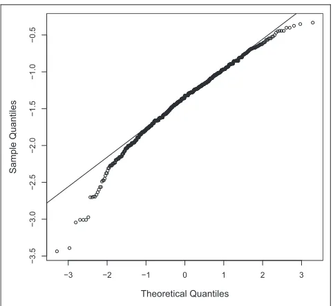
The analytic method for computing the inner con-ditional expectation EujxfNBðd;uÞg is exact for sce-nario 1 but not for scesce-narios 2 and 3. In scesce-narios 2 and 3, a Taylor series approximation is used to derive the expectation of a logit-transformed parameter from the expectation of the parameter itself, and in sce-nario 3, the log odds ratio obtained for each simulated study is assumed to be Normally distributed. These approximations are not required in either the 2-level method or the regression method. The assumption in the analytic method that the study log odds ratios are Normally distributed may in particular be problem-atic. The assumption is reasonable if the underlying probabilities are close to 0.5 but not when probabili-ties are close to 0 or 1. In our case study, the mean probability of a critical event is EðPTÞ50:044 on the new treatment and EðPCÞ50:15 on standard
care. To explore the robustness of the assumption of Normality, we generated samples from XT ~
Binom(0.044, 200) and XC ~ Binom(0.15, 200) and,
[image:11.594.48.289.91.313.2]for each pair of samples, calculated the log odds ratio. A Normal QQ plot of the sampled log odds ratios in
Figure 3 shows that the assumption of Normality does not hold.
Precision and Computational Efficiency
For comparisons within each method, the Monte Carlo standard error scales in proportion to K21/2
(as expected), and the computation time scales approximately in proportion toK.
For the same level of precision, the 2-level Monte Carlo method requires 104(i.e., the inner loop size) times as many samples as does the Ades et al.7 ana-lytic method. This holds across all 3 scenarios. The 2-level method is roughly 5 orders of magnitude slower than the Ades et al. method for the same value ofK, primarily due to the requirement for 104model evaluations at each outer-loop run.
For scenario 1, the standard errors obtained using the GAM method are approximately 20% larger than those of the analytic method, given the same number of model runs. Thus, to achieve the same pre-cision, the number of runs would need to be increased by approximately 1.22 = 1.44 times (this was con-firmed empirically; results not shown). For scenario 2, the standard errors obtained using the GAM method are approximately 4 times larger than those of the ana-lytic method, given the same number of model runs. Thus, to achieve the same precision, the number of runs would need to be increased by approximately 16 times. For scenario 3, the standard errors obtained using the GAM method are approximately 60% larger than those of the analytic method, given the same number of model runs. Here, to achieve the same pre-cision, the number of runs would need to be increased by approximately 2.6 times.
The precision of the GAM estimate, as well as being related to the sample size, is related to the uncertainty in the model parameters that are not updated by the data. This uncertainty propagates through to the model output (the net benefit) in the PSA sample and causes the variability in the net ben-efit that is modeled by the error term in the regression. In the case of scenario 2, the GAM estimate requires relatively more samples (for some given precision) than does the GAM estimate for scenario 1 or 3. This suggests that in scenario 2, the uncertainty in the parameters not updated by data (i.e., PSE and
log(OR)) is large. This is confirmed by the relatively high partial EVPI values forPSEand log(OR).
In terms of computational speed, the GAM method is roughly an order of magnitude slower than the
−3 −2 −1 0 1 2 3
−3.5
−3.0
−2.5
−2.0
−1.5
−1.0
−0.5
Theoretical Quantiles
Sample Quantiles
analytic method but roughly 4 orders faster than the 2-level method.
DISCUSSION
Our key idea is that instead of estimating, for each decision option, the posterior expected net benefits via a computationally burdensome repeated (inner-loop) Monte Carlo step, we estimate the functional rela-tionship between the posterior expected net benefit and the simulated data via a nonparametric regression.
Strengths and Limitations
The value of the nonparametric regression method over the 2-level Monte Carlo approach is 2-fold: it is straightforward to implement, requiring less detailed mathematical thinking on the part of the analyst for any particular application, and is several orders of magnitude faster for any given precision. Due to the method’s ease of use and the fact that it only requires the PSA sample and not the model itself, we would suggest that the regression method is applicable in even the simplest of modeling contexts.
In common with other established methods for computing EVSI, we must be able to generate sample data sets, conditional on samples from the prior dis-tribution of the model parameters. For complex study designs, this may not be straightforward. For our method, we must also be able to summarize the sam-pled data in either a scalar, or low-dimensional, sum-mary statistic. Again, for complex study designs, this may not always be easy.
How This Fits with Existing Literature
One option for computing EVSI is to assume that the incremental net benefit is Normally distributed with parameters that are known functions of study sample size. Under this assumption, EVSI can be cal-culated using fast analytical methods. This ‘‘paramet-ric’’ approach is most appropriate in settings in which cost-effectiveness analysis is undertaken alongside a single 2-arm randomized controlled trial (RCT). In this setting, the mean incremental net ben-efit is derived directly from individual-level costs and effects, and the central limit theorem can be used to justify the assumption of Normality. The method has been explored in theoretical investi-gations9–13and applied in real clinical decision prob-lems.30However, the approach is not straightforward for decision problems with more than 2 options and
may not be appropriate when a more complex decision-analytic model has been used to estimate incremental net benefit. A nonlinear cost-effectiveness model with non-Normal input parameters may gener-ate notably non-Normal incremental net benefits. It may be difficult to predict the relationship between the size of a proposed study that informs some partic-ular subset of parameters and the net benefits of a range of competing decision options. Deriving the parame-ters of the Normal distribution(s) that the parametric approach requires may therefore be difficult.
The nonparametric regression approach that we propose has some similarities to the model emulation method proposed in Oakley,31and in one sense, the GAM model can be viewed as an emulator for the pos-terior expectation of the net benefit, conditional on the data. The important difference between the 2 approaches is that in Oakley, the net benefit function itself is emulated. Emulating the net benefit function allows for the rapid evaluation of a slow economic model, but it does not address the problem of how to sample from a difficult posterior distribution of the parameters conditional on the data. Our method also has some similarities to the spline-based approach for computing partial EVPI that has been proposed by Madan et al.21Here, a spline is used to approximate the conditional expectation of some pre-defined subfunction of the net benefit function, given some sampled value of a parameter of interest. Although the method by Madan et al is shown to per-form well, it requires algebraic manipulation of the net benefit function to identify the appropriate sub-functions for the spline approximation. This may be difficult in complex models.
Implications for Practice and for Research
Throughout the article, we have assumed that the decision maker’s utility is equal to net benefit and that the decision problem is to maximize net benefit over a set of discrete treatment options. This is the typical decision problem faced by government agen-cies such as the National Institute for Health and Care Excellence (NICE), but the type of decision prob-lem faced by the pharmaceutical industry is some-what different. Here, utility is profit, and under value-based pricing, the decision problem is to choose price to maximize profit, subject to the con-straint that additional health benefits do not cost more than the funder’s willingness to pay. EVSI from an industry perspective has been explored by Willan34and by Willan and Eckermann,35as well as more recently within a value-based pricing context by Breeze and Brennan.36Our nonparametric
regres-sion method for computing EVSI will apply equally well in this context.
Further research could extend to testing the nonparametric regression method in other cost-effectiveness models, including Markov cohort mod-els and more complex patient-level modmod-els. An important feature of our method is that all variation in the net benefit function that is not due to the data is taken up by the error term in the regression analysis and ‘‘averaged out.’’ Thus, any variation in the net benefit that arises due to poor convergence of a patient-level model is also averaged out in the regression.24 This means that, to calculate EVSI for a patient-level model (in which patients do not inter-act), only a single patient needs to be ‘‘run’’ through the model at each evaluation of the PSA. We look for-ward to more research in this area.
REFERENCES
1. Eckermann S, Willan AR. Expected value of information and decision making in HTA. Health Econ. 2007;16(2):195–209. 2. McKenna C, Claxton K. Addressing adoption and research design decisions simultaneously. Med Decis Making. 2011;31(6): 853–65.
3. Raiffa H. Decision Analysis. Introductory Lectures on Choices under Uncertainty. Reading, MA: Addison-Wesley; 1968. 4. Claxton K, Posnett J. An economic approach to clinical trial design and research priority-setting. Health Econ. 1996;5(6):513–24. 5. Felli JC, Hazen GB. Sensitivity analysis and the expected value of perfect information. Med Decis Making. 1998;18(1):95–109. 6. Felli JC, Hazen GB. Erratum: Correction: sensitivity analysis and the expected value of perfect information. Med Decis Making. 2003;23(1):97.
7. Ades AE, Lu G, Claxton K. Expected value of sample informa-tion calculainforma-tions in medical decision modeling. Med Decis Mak-ing. 2004;24(2):207–27.
8. Eckermann S, Karnon J, Willan AR. The value of value of infor-mation: best informing research design and prioritization using current methods. Pharmacoeconomics. 2010;28(9):699–709. 9. Eckermann S, Willan AR. The option value of delay in health technology assessment. Med Decis Making. 2008;28(3):300–5. 10. Eckermann S, Willan AR. Time and expected value of sample information wait for no patient. Value Health. 2008;11(3):522–6. 11. Willan AR, Eckermann S. Optimal clinical trial design using value of information methods with imperfect implementation. Health Econ. 2010;19(5):549–61.
12. Eckermann S, Willan AR. Globally optimal trial design for local decision making. Health Econ. 2009;18(2):203–16.
13. Eckermann S, Willan AR. Optimal global value of information trials: better aligning manufacturer and decision maker interests and enabling feasible risk sharing. Pharmacoeconomics. 2013; 31(5):393–401.
14. Claxton K. Bayesian approaches to the value of information: implications for the regulation of new pharmaceuticals. Health Econ. 1999;8(3):269–74.
15. Claxton K. The irrelevance of inference: a decision-making approach to the stochastic evaluation of health care technologies. J Health Econ. 1999;18(3):341–64.
16. Soares MO, Dumville JC, Ashby RL, et al. Methods to assess cost-effectiveness and value of further research when data are sparse: negative-pressure wound therapy for severe pressure ulcers. Med Decis Making. 2013;33(3):415–36.
17. Brennan A, Kharroubi SA. Expected value of sample informa-tion for Weibull survival data. Health Econ. 2007;16(11):1205–25. 18. Brennan A, Kharroubi SA. Efficient computation of partial expected value of sample information using Bayesian approxima-tion. J Health Econ. 2007;26(1):122–48.
19. Kharroubi SA, Brennan A, Strong M. Estimating expected value of sample information for incomplete data models using Bayesian approximation. Med Decis Making. 2011;31(6):839–52. 20. Welton NJ, Madan JJ, Caldwell DM, Peters TJ, Ades AE. Expected value of sample information for multi-arm cluster randomized trials with binary outcomes. Med Decis Making. 2014;34(3):352–65. 21. Madan J, Ades AE, Price M, et al. Strategies for efficient com-putation of the expected value of partial perfect information. Med Decis Making. 2014;34(3):327–42.
22. Strong M, Oakley JE. An efficient method for computing sin-gle-parameter partial expected value of perfect information. Med Decis Making. 2013;33(6):755–66.
23. Sadatsafavi M, Bansback N, Zafari Z, Najafzadeh M, Marra C. Need for speed: an efficient algorithm for calculation of single-parameter expected value of partial perfect information. Value Health. 2013;16(2):438–48.
24. Strong M, Oakley JE, Brennan A. Estimating multi-parameter partial expected value of perfect information from a probabilistic sensitivity analysis sample: a non-parametric regression approach. Med Decis Making. 2014;34(3):311–26.
25. Lunn D, Spiegelhalter D, Thomas A, Best N. The BUGS project: evolution, critique, and future directions. Stat Med. 2009;28(25): 3049–67.
27. Hastie T, Tibshirani R. Generalized additive models. Stat Sci. 1986;1(3):297–318.
28. Wood SN. Generalized Additive Models: An Introduction with R. Boca Raton, FL: Chapman and Hall/CRC; 2006.
29. Gelman A, Hill J. Data Analysis Using Regression and Multi-level/Hierarchical Models. New York: Cambridge University Press; 2007.
30. Kent S, Briggs A, Eckermann S, Berry C. Are value of informa-tion methods ready for prime time? An applicainforma-tion to alternative treatment strategies for NSTEMI patients. Int J Technol Assess Health Care. 2013;29(4):435–42.
31. Oakley JE. Decision-theoretic sensitivity analysis for complex computer models. Technometrics. 2009;51(2):121–9.
32. Soares MO, Welton NJ, Harrison DA, et al. An evaluation of the feasibility, cost and value of information of a multicentre rando-mised controlled trial of intravenous immunoglobulin for sepsis (severe sepsis and septic shock): incorporating a systematic
review, meta-analysis and value of information analysis. Health Technol Assess. 2012;16(7):1–186.
33. Leaviss J, Sullivan W, Ren S, et al. What is the clinical effec-tiveness and cost-effeceffec-tiveness of cytisine compared with vareni-cline for smoking cessation? A systematic review and economic evaluation. Health Technol Assess. 2014;18(33):1–120.
34. Willan AR. Optimal sample size determinations from an industry perspective based on the expected value of information. Clin Trials. 2008;5(6):587–594.
35. Willan AR, Eckermann S. Value of information and pricing new healthcare interventions. Pharmacoeconomics. 2012;30(6):447–59. 36. Breeze P, Brennan A. Valuing trial designs from a pharmaceu-tical perspective using value-based pricing [published online Sep-tember 9, 2014]. Health Econ.