The RMS survey: ammonia mapping of the environment of massive young
stellar objects
J. S. Urquhart,
1‹C. C. Figura,
2‹T. J. T. Moore,
3‹T. Csengeri,
1S. L. Lumsden,
4T. Pillai,
1M. A. Thompson,
5D. J. Eden
6and L. K. Morgan
3,71Max-Planck-Institut f¨ur Radioastronomie, Auf dem H¨ugel 69, D-53121 Bonn, Germany 2Wartburg College, 100 Wartburg Blvd, Waverly, IA 50677, USA
3Astrophysics Research Institute, Liverpool John Moores University, 146 Brownlow Hill, Liverpool L3 5RF, UK 4School of Physics and Astrophysics, University of Leeds, Leeds LS2 9JT, UK
5Centre for Astrophysics Research, Science and Technology Research Institute, University of Hertfordshire, College Lane, Hatfield AL10 9AB, UK 6Observatoire astronomique de Strasbourg, Universite de Strasbourg, CNRS, UMR 7550, 11 rue de l’Universit, F-67000 Strasbourg, France 7Met Office, FitzRoy Road, Exeter, Devon EX1 3PB, UK
Accepted 2015 July 6. Received 2015 July 6; in original form 2015 May 26
A B S T R A C T
We present the results of ammonia observations towards 66 massive star forming regions identified by the Red Midcourse Space Experiment Source survey. We have used the Green Bank Telescope and the K-Band Focal Plane Array to map the ammonia (NH3) (1,1) and (2,2)
inversion emission at a resolution of 30 arcsec in 8 arcmin regions towards the positions of embedded massive star formation. We have identified a total of 115 distinct clumps, approximately two-thirds of which are associated with an embedded massive young stellar object or compact HIIregion, while the others are classified as quiescent. There is a strong
spatial correlation between the peak NH3emission and the presence of embedded objects. We
derive the spatial distribution of the kinetic gas temperatures, line widths, and NH3 column
densities from these maps, and by combining these data with dust emission maps we estimate clump masses, H2column densities and ammonia abundances. The clumps have typical masses
of∼1000 Mand radii∼0.5 pc, line widths of∼2 km s−1and kinetic temperatures of∼16–
20 K. We find no significant difference between the sizes and masses of the star-forming and quiescent subsamples; however, the distribution maps reveal the presence of temperature and line width gradients peaking towards the centre for the star-forming clumps while the quiescent clumps show relatively uniform temperatures and line widths throughout. Virial analysis suggests that the vast majority of clumps are gravitationally bound and are likely to be in a state of global free fall in the absence of strong magnetic fields. The similarities between the properties of the two subsamples suggest that the quiescent clumps are also likely to form massive stars in the future, and therefore provide an excellent opportunity to study the initial conditions of massive pre-stellar and protostellar clumps.
Key words: stars: early-type – stars: formation – ISM: molecules – radio lines: ISM.
1 I N T R O D U C T I O N
Although massive stars (>8 M and 103 L
) make up only a few per cent of the stellar population, they play a central role in many astrophysical processes. They have a profound impact on their local environments through powerful outflows, strong stellar winds, copious amounts of optical/far-UV radiation, and chemi-cal enrichment. The energy and processed material returned to the
∗E-mail: [email protected] (JSU); [email protected]
(CCF);[email protected](TJTM)
interstellar medium (ISM) play an important role in regulating star formation by changing the local chemistry and through the propa-gation of strong shocks in the surrounding molecular clouds. These feedback processes may be responsible for triggering subsequent generations of stars to form or disrupting conditions necessary for star formation in nearby clouds (Elmegreen1998), ultimately gov-erning the evolution of their host galaxy (Kennicutt2005).
Despite their importance, our understanding of the initial con-ditions required and processes involved in the formation and early evolution of massive stars is still rather poor. There are a number of reasons for this: massive stars are rare and relatively few are located closer than a few kiloparsecs; they form almost exclusively
2015 The Authors
at University of Leeds on March 30, 2016
http://mnras.oxfordjournals.org/
in clusters, making it hard to distinguish between the properties of the cluster and individual members; and they evolve rapidly, reaching the main sequence while still deeply embedded in their natal environment, and consequently the earliest stages can only be probed at far-infrared, (sub)millimetre and radio wavelengths. Previous studies have been limited to high angular resolution obser-vations of specific objects or larger low-resolution surveys which have tended to focus on bright far-infrared and/or radio sources that are already very luminous (>103L
; e.g. Wood & Churchwell
1989; Molinari et al.1996; Sridharan et al.2002). These studies
have identified a large number of young massive stars; however, source confusion in complex regions resulted in these samples be-ing biased away from the Galactic mid-plane where the majority of massive stars are located (scaleheight∼30 pc; Reed2000). It is therefore unclear whether these samples are a good representation of the global population of young massive stars.
The Red MSX Source (RMS; Lumsden et al.2013) survey has used a combination of Midcourse Space Experiment (MSX) and Two Micron All-Sky Survey (2MASS) point source catalogues to identify an unprecedented sample of candidate embedded massive young stars. A multiwavelength campaign of follow-up observa-tions (Mottram et al.2007; Urquhart et al.2007a,b,2008,2009a,b,
2011; Cooper et al.2013) has led to the identification of a
combi-nation of∼1300 massive young stellar objects (MYSOs) and com-pact HIIregions (Lumsden et al.2013). This is the largest and most
well-characterized sample yet compiled, and is an order of magni-tude larger than previous catalogues. In a recent study (Urquhart et al.2014b), we investigated the bulk properties of these massive star-forming (MSF) regions using the submillimetre dust emission traced by the APEX Telescope Large Area Survey of the Galaxy (ATLASGAL) survey (870µm; Schuller et al.2009). We extracted clumps parameters by matching the positions of the RMS catalogue with the ATLASGAL Compact Source Catalogue (CSC; Contr-eras et al.2013; Urquhart et al.2014c). This study found strong correlations between the clump mass and the bolometric luminos-ity of the embedded source, and between clump mass and radius (partial Spearman correlation coefficientsrAB, C =0.64 and 0.85,
respectively; see Section 4.1 for definition); however, the available continuum data was not sufficient to investigate these correlations in detail.
In this paper, we use a flux-limited sample of RMS sources to investigate the properties of their natal clumps and the role that environmental conditions play in the formation of massive stars. We have mapped 66 MSF regions in the lowest excitation ammonia inversion transitions (i.e. NH3(J,K)=(1,1) and (2,2)). These
transi-tions are sensitive to cold (∼10–40 K; Ho & Townes1983; Mangum, Wootten & Mundy1992) and dense (>104cm−3; Rohlfs & Wilson
2004) gas and NH3 does not deplete from the gas phase at high
densities (<106cm−3; Bergin & Langer1997), which makes them
an excellent probe of the dense gas properties of these clumps (Rydbeck et al.1977; Ho & Townes1983). Furthermore, the ratio of the hyperfine components of the NH3(1,1) can be used to
esti-mate the optical depth and relative populations of different levels, which can be used to estimate the rotation and kinetic temperature of the gas.
Ammonia is therefore one of the most useful high-density molec-ular gas tracers, and has been widely used to study the properties of MSF regions. These studies have sampled a range of evolu-tionary stages such as infrared dark clouds (IRDCs; Pillai et al.
2006; Ragan, Bergin & Wilner2011; Chira et al.2013), massive
submillimetre clumps (Dunham et al. 2011; Wienen et al.2012) and embedded mid-infrared bright sources (Urquhart et al.2011;
hereafterPaper I). These have found that higher temperatures and larger line widths tend to be associated with more evolved proto-stars, which is generally attributed to increased feedback from the embedded objects.
We used these observations to trace the temperature and density structure of these MSF environments and probe the gas kinemat-ics, which in turn provides an insight into the bulk motion of the gas and level of turbulence, and through virial analysis, an estimate of the global stability of these clumps. These data are combined with archival infrared and submillimetre data to investigate the re-lationship between the embedded MYSOs and compact HIIregions
and their natal clumps, and to evaluate the influence of the local environment on the structure and evolution of the clumps.
The combined data set is extremely rich and will form the foun-dation for several studies. In this paper, the second in the series, we present the results of ammonia mapping observations and a sta-tistical analysis of the mean clump parameters. Subsequent papers will focus on the relationship between the larger-scale environ-ment and the dense clumps, the density and temperature structure of the clumps, and detailed studies of more complicated regions. The structure of the paper is as follows: in Section 2, we describe the observational set-up, data reduction and source extraction pro-cedures, as well as the spectral line analysis. In Section 3, we present an overview of our results, derive physical properties for the clumps and compare their distributions with respect to their em-bedded protostellar content, and evaluate the impact of the external environment. We investigate the correlation between different de-rived properties in Section 4. We summarize our results and present our conclusions in Section 5.
2 O B S E RVAT I O N S A N D DATA A N A LY S I S
2.1 GBTK-band mapping observations
We have mapped 62 fields towards MYSOs and compact HIIregions
identified by the RMS survey. A further four fields were included towards strong dust emission sources that are not associated with an RMS source to allow comparison between MSF clumps and relatively quiescent clumps. These observations have been made using the K-Band Focal Plane Array (KFPA) on the National Radio Astronomy Observatory’s1Green Bank Telescope (GBT). The
ob-servations were made in shared-risk time shortly after the KFPA was commissioned between 2011 March and 2012 February (Project Id.: GBT10C21).
The fields were selected using the results of a programme of tar-geted observations also made with the GBT towards∼600 RMS sources (Paper I). This previous study detected NH3emission
to-wards approximately 80 per cent of the sources targeted. We have selected bright sources that have good detections in both ammonia transitions in order to provide the highest sensitivity maps of the various parameters (e.g.vLSR, line width, density and temperature)
and trace their spatial distribution across these star-forming regions. We chose to focus on sources located within the inner Galactic plane (i.e. <60◦and|b|<1◦) as this has been covered by a number of other surveys and ensures the availability of a wealth of comple-mentary data. It was not always possible to meet these two criteria
1The National Radio Astronomy Observatory is a facility of the National Science Foundation operated under cooperative agreement by Associated Universities, Inc.
at University of Leeds on March 30, 2016
http://mnras.oxfordjournals.org/
simultaneously and as a result a few fields were observed outside this region.
The KFPA features seven 32 arcsec beams in a hexagonal array with a central feed, with a nearest neighbour spacing of 96 arcsec. A 50 MHz spectral bandpass was used to observe both of the ammo-nia (1,1) and (2,2) rotation inversion transitions simultaneously (at ∼23.6945 and 23.7226 GHz, respectively). The ‘Daisy’ pattern was used to map a region∼8 arcmin in diameter towards each target source. The petal-shaped scan trajectories produce fully sampled maps within a radius of 3.5 arcmin of map centre; beyond this point the integration time decreases, resulting in a decrease in signal-to-noise ratios (SNR) towards the map edges. Maps were weighted by integration times during the data reduction in order to compensate for this decrease.
Sky subtraction was accomplished via off-source observations, and a noise diode was used to calibrate fluxes to theTA∗scale. The zenith atmospheric opacity was determined using weather models.2
Time series data from the seven individual receivers in the array was processed through the GBT reduction pipeline.3Sky subtraction
and calibration was performed by the pipeline, and spatial image cubes were produced. The weather conditions were stable for all observations, and the typical pointing corrections were found to be ∼4 arcsec.
The reduced data cubes are approximately 8 arcmin in diameter and gridded using 6 arcsec pixels. All maps were smoothed spatially with a 10 arcsec Gaussian kernel, which results in a final image res-olution of∼32 arcsec, while the velocity axis was smoothed using a top-hat function to produce a resolution of∼0.4 km s−1channel−1.
In a few cases where the observed fields overlapped the adjacent maps were mosaicked together using thewcsmosaicroutine from the StarlinkKAPPAsuite to maximize the fully sampled region.4In
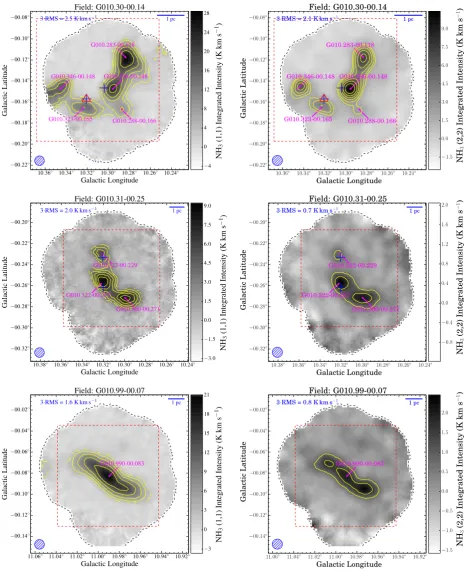
Fig.1, we present a selection of integrated NH3 (1,1) and (2,2)
emission maps for three fields. The contour levels start at 3σ and increase in steps set by a dynamically determined power law of the formD=3×Ni+2, whereDis the dynamic range of the submil-limetre emission map (defined as the peak brightness divided by the local rms noise),Nis the number of contours used (6 in this case), andiis the contour power-law index. The lowest power-law index used was one, which results in linearly spaced contours starting at 3σ and increasing in steps of 3σ (see Thompson et al.2006for more details). The complete set of maps are provided in Fig. A1. In Table1, we give the names, centre coordinates, the noise in the integrated maps of the observed fields along with the distance and velocities of the target sources.
2.2 Source extraction and structure analyses
The emission maps reveal a mixture of isolated clumps with rather simple elliptical distributions and a smaller number of more irreg-ular multipeaked morphologies that are likely to consist of two or more distinct clumps. We have used theFellWalkersource ex-traction algorithm (Berry2015) to identify clumps and determine their properties in a consistent manner.5This algorithm has been
applied to the integrated NH3(1,1) emission maps as they have the
2http://www.gb.nrao.edu/rmaddale/Weather.
3https://safe.nrao.edu/wiki/pub/Kbandfpa/KfpaReduction/
kfpaDataReduceGuide-11Dec01.pdfsee also Morgan et al. (2014). 4http://www.starlink.ac.uk/docs/sun95.htx/sun95.html
5FellWalkeris part of theSTARLINK-CUPIDsoftware suite and more details can be found here:http://docs.jach.hawaii.edu/star/sun255.htx/sun255.html.
highest sensitivity and will most accurately trace the full extent of the clumps.
We set a 3σ detection threshold and required that all sources identified consist of more than 30 pixels in order to reject sources with fewer pixels than the beam integral as these are likely to be spurious detections. We also excluded clumps located towards the edges of the fields as these tend to have lower SNRs, and it is likely that the emission is not entirely captured in the maps leading to larger uncertainties. Multiple clumps are found in 35 of the 66 observed fields (11 fields have three clumps, and one has five clumps; the number of clumps identified in each field is given in Table 1). In the majority of cases, clumps found in the same field have similar radial velocities (typically differing by less than a few km s−1) and are therefore likely to be associated with the
same giant molecular cloud (GMC) complex and can be assumed to be at a similar distance. There are only two fields where the clumps are at significantly different velocities (G024.18+00.12 and G028.29−00.38). We will discuss these two fields in more detail in Section 3.5.1. In fields where two or more clumps are identified, we find that the RMS source is nearly always associated with the brightest and most prominent of the clumps identified.
In total, 115 clumps have been detected and these are identified by labels on the emission maps presented in Fig.1and their parameters are given in Table2. The source names are based on the Galactic coordinates of the peak flux position, which are given in Columns 2 and 3. The source sizes describe an ellipse with semimajor and semiminor axis lengths and position angle; these are determined from the standard deviation of the pixel coordinate values about the centroid position weighted by the pixel values (seeCUPIDmanual
for more details).
The ratio of the semimajor and semiminor axes is used to estimate the aspect ratio of each source, which in turn is used to classify each clump into one of two groups: spheroidal and filamentary structures. In Fig.2, we present the cumulative distribution of the aspect ratio for all of the clumps. This plot shows a break at an aspect ratio of approximately 1.8 and we used this value to distinguish between spheroids and filaments, with the former having smaller aspect ra-tios. This results in 94 spheroidal and 21 filamentary structures. The fraction of filaments identified is significantly lower than has been found for several other high-resolution ammonia surveys (i.e. almost ubiquitous by Lu et al.2014at 3–40 arcsec and over 50 per cent by Ragan et al.2011at 4 and 8 arcsec resolution). It is therefore ex-pected that many of the spheroidally structured clumps will turn out to be filamentary at higher resolution, but the sources classified as filamentary are unlikely to be affected and so this may prove a useful distinction. We investigated the possibility that sources that were identified as filamentary were more likely to be closer and thus more easily resolved. There was, however, no statistically sig-nificant difference between filamentary and spheroidal subsample distances, indicating that filaments can have a large range of size scales.
The clump position angle is given as anticlockwise from Galactic north. In Fig.3, we show the difference between the clump position angles and the Galactic mid-plane. It is clear from this plot that the clumps are preferentially aligned along the Galactic mid-plane, suggesting that Galactic rotation, magnetic field, or Galactic shear may be influencing their structure, although the last of these is less likely (Dib et al.2012). We find no correlation between the clump orientation and the angular separation from the Galactic mid-plane (i.e.|b|). Li et al. (2014) present evidence that the B-field in cores is aligned with the local large-scale field in the diffuse ISM and that the latter is in turn aligned with the Galactic plane.
at University of Leeds on March 30, 2016
http://mnras.oxfordjournals.org/
Figure 1. Examples of the integrated NH3 (1,1) and (2,2) emission maps obtained towards three fields are presented on the left- and right-hand panels, respectively. The NH3(1,1) emission is integrated over a velocity range of∼50 km s−1in order to include the main line and four hyperfine components and is centred on the velocity of the central clump in each field. The NH3(1,1) emission is integrated over a velocity range of three times the standard deviation of the Gaussian fit to the peak profile. The grey-scale and yellow contours show the distribution of the integrated emission. The positions of the MYSOs, HIIregions and MYSO/HIIregions are indicated by blue crosses, red triangles and purple squares, respectively. The dashed red lines outline the regions we focus on in Figs6and9. The contour levels start at 3σand increase in steps set by a dynamically determined power law (see the text for details). The 3σ noise is given in the top-left corner and a linear scale bar shown in the upper-right corner provides an indication of the physical sizes of the clumps. The angular resolution of the GBT beam at this frequency is indicated by the blue hatched circle shown in the lower-left corner of each map. Only a small portion of the data is provided here, the full figure is only available in electronic form at the CDS via anonymous ftp to cdsarc.u-strasbg.fr (130.79.125.5) or via
http://cdsweb.u-strasbg.fr/cgi-bin/qcat?J/A+A/.
at University of Leeds on March 30, 2016
http://mnras.oxfordjournals.org/
Table 1. Observed field parameters.
Field Field RA Dec. Map sensitivity Number vLSR Distance
Id name (J2000) (J2000) (K km s−1) of clumps (km s−1) (kpc)
1 G010.300−00.143 18:08:54.88 −20:05:51.1 0.82 5 12.9 2.2
2 G010.315−00.251 18:09:20.89 −20:08:10.1 0.66 3 27.7 4.0
3 G010.472+00.033 18:08:36.89 −19:51:40.1 0.62 2 67.1 8.5
4 G010.648−00.342 18:10:22.41 −19:53:19.5 1.98 3 −5.0 4.9
5 G010.990−00.075 18:10:04.88 −19:27:37.4 0.54 1 29.7 3.7
6 G011.112−00.395 18:11:31.25 −19:30:29.1 0.64 3 −1.0 4.9
7 G011.501−01.482 18:16:21.87 −19:41:10.5 0.56 2 10.6 1.6
8 G011.902−00.135 18:12:09.88 −18:41:25.4 0.67 3 36.4 12.8
9 G011.924−00.613 18:13:58.89 −18:53:59.2 0.78 1 35.2 3.9
10 G012.432−01.111 18:16:51.25 −18:41:29.4 0.36 2 – 4.1
11 G012.887+00.494 18:11:50.25 −17:31:27.2 0.54 3 33.5 2.4
12 G013.197−00.122 18:14:43.63 −17:32:52.1 1.47 2 53.1 4.6
13 G013.330−00.034 18:14:40.26 −17:23:18.1 0.42 2 54.7 4.7
14 G013.656−00.595 18:17:23.25 −17:22:09.2 0.51 1 47.0 4.3
15 G013.873+00.282 18:14:35.63 −16:45:39.0 0.53 1 48.5 4.4
16 G014.330−00.639 18:18:53.25 −16:47:46.3 0.67 1 22.0 1.1
17 G014.433−00.697 18:19:18.26 −16:43:57.4 0.60 1 16.9 1.1
18 G014.608+00.019 18:17:01.10 −16:14:21.0 0.48 2 25.1 2.9
19 G016.711+01.318 18:16:25.27 −13:46:18.3 0.48 1 20.0 2.2
20 G016.804+00.817 18:18:25.26 −13:55:38.4 0.51 1 – 2.1
21 G016.927+00.961 18:18:08.28 −13:45:03.1 0.70 1 20.9 2.2
22 G017.451+00.813 18:19:41.65 −13:21:34.0 0.41 1 21.3 2.2
23 G017.636+00.156 18:22:26.27 −13:30:21.3 0.59 2 22.1 2.2
24 G018.301−00.387 18:25:41.27 −13:10:20.4 0.58 1 32.3 3.0
25 G018.461+00.001 18:24:35.27 −12:50:58.4 0.62 1 52.4 12.1
26 G018.606−00.071 18:25:07.64 −12:45:19.1 0.61 3 46.0 3.7
27 G018.662+00.030 18:24:52.00 −12:39:28.9 0.56 1 80.9 10.8
28 G018.846−00.558 18:27:21.06 −12:46:11.3 0.87 2 65.2 4.5
29 G019.078−00.285 18:26:48.28 −12:26:12.2 0.62 1 66.0 4.5
30 G019.756−00.130 18:27:32.00 −11:45:54.9 0.53 2 60.2 4.3
31 G019.885−00.535 18:29:14.64 −11:50:21.2 0.59 1 43.2 3.5
32 G019.923−00.258 18:28:19.00 −11:40:36.8 0.63 1 64.7 4.5
33 G020.747−00.074 18:29:12.64 −10:51:41.1 0.60 3 56.0 4.2
34 G021.373−00.241 18:30:59.63 −10:23:01.2 0.59 2 90.8 10.3
35 G022.350+00.070 18:31:42.64 −09:22:26.0 0.62 1 84.2 5.2
36 G022.414+00.315 18:30:56.99 −09:12:16.0 0.61 3 84.2 5.2
37 G023.708+00.172 18:33:52.99 −08:07:21.0 0.60 3 113.0 9.1
38 G024.183+00.120 18:34:57.01 −07:43:28.8 0.63 3 54.5 3.8
39 G025.649+01.047 18:34:21.36 −05:59:46.6 0.67 2 42.2 3.1
40 G025.716+00.046 18:38:03.36 −06:23:49.6 0.58 1 99.2 9.5
41 G025.815−00.168 18:39:00.35 −06:24:28.7 0.60 1 93.7 5.0
42 G027.269+00.147 18:40:33.35 −04:58:15.7 0.71 2 31.6 12.8
43 G028.199−00.049 18:42:58.00 −04:14:00.9 0.58 2 98.2 5.9
44 G028.293−00.377 18:44:18.35 −04:17:59.6 0.70 2 48.8 11.6
45 G028.337+00.113 18:42:38.35 −04:02:10.7 0.84 1 81.0 5.0
46 G029.596−00.615 18:47:32.34 −03:14:56.8 0.76 2 76.6 4.8
47 G030.877+00.056 18:47:29.35 −01:48:09.6 0.56 2 74.5 4.9
48 G031.271+00.061 18:48:11.35 −01:26:59.7 0.80 2 109.0 4.9
49 G031.406+00.299 18:47:35.35 −01:13:15.6 0.56 1 97.6 4.9
50 G032.052+00.068 18:49:35.35 −00:45:08.8 0.81 1 95.3 4.9
51 G033.397−00.001 18:52:17.35 +00:24:48.2 0.55 1 103.9 7.1
52 G033.913+00.109 18:52:50.35 +00:55:23.1 0.48 1 107.5 7.1
53 G034.407+00.231 18:53:18.35 +01:25:06.2 0.68 1 57.9 3.8
54 G035.196−00.744 18:58:12.99 +01:40:29.9 0.50 2 33.9 2.2
55 G035.463+00.140 18:55:33.35 +02:18:58.3 0.53 1 74.1 8.8
56 G037.554+00.201 18:59:09.99 +04:12:13.9 0.48 1 85.1 6.7
57 G043.180−00.520 19:12:09.36 +08:52:11.3 0.49 2 57.5 8.2
58 G043.306−00.213 19:11:17.36 +09:07:26.3 0.48 1 59.6 4.4
59 G045.462+00.049 19:14:24.36 +11:09:20.1 0.56 1 62.1 6.7
60 G048.989−00.301 19:22:26.36 +14:06:33.1 0.55 2 71.0 5.6
61 G052.204+00.724 19:25:00.27 +17:25:34.8 0.54 3 0.5 –
62 G053.604+00.015 19:30:25.88 +18:19:06.5 0.52 2 25.3 1.9
63 G058.468+00.437 19:38:57.00 +22:46:32.1 0.53 2 36.4 4.4
at University of Leeds on March 30, 2016
http://mnras.oxfordjournals.org/
Table 1 –continued
Field Field RA Dec. Map sensitivity Number vLSR Distance
Id name (J2000) (J2000) (K km s−1) of clumps (km s−1) (kpc)
64 G059.782+00.075 19:43:08.62 +23:44:18.9 0.50 1 22.3 2.2
65 G075.766+00.358 20:21:37.30 +37:26:20.9 0.54 2 – 1.4
66 G078.977+00.363 20:31:09.48 +40:03:30.3 0.49 1 – 1.4
The orientation of the elongation of the cores is then aligned either parallel or perpendicular to the direction of the B-field. It therefore seems likely that the preferred orientation of the clumps is due to the influence of large-scale magnetic fields, or that perhaps both are influenced by Galactic kinematics.
The source sizes are only determined from pixels above the de-tection threshold and are therefore likely to underestimate the true source sizes. This can sometimes result in sizes that are smaller than the full width at half-maximum (FWHM) of the telescope beam as the moment method of determining sizes truncates the low-significance emission in the clump’s outer envelope (cf. Rosolowsky et al.2010; Section 7.4). We estimate the angular radius (θR) from
the geometric mean of the deconvolved major and minor axes, mul-tiplied by a factorηthat relates the rms size of the emission distri-bution of the source to its angular radius (equation 6 of Rosolowsky et al.2010):
θR=η
(σ2
maj−σ 2 bm)(σ
2 min−σ
2 bm)
1/4
, (1)
whereσbmis the rms size of the beam (i.e.σbm=θFWHM/
√ 8 ln 2 13 arcsec). Following Rosolowsky et al. (2010), we adopt a value forηof 2.4 to estimate the effective radius of each source. We are able to estimate the effective radius for all but eight clumps: these eight have at least one of their axes smaller than the beamwidth; however, all of these are relatively weak (SNR∼8) and it is likely that the observations do not trace the full extent of their extended envelopes.
The peak flux is directly obtained fromFellWalker; however, the integrated emission is the sum of all pixels above the threshold and does not take account of the beam size. To obtain a value for the total emission, we have divided the derived flux by the beam integral (i.e. 1.133×FWHM232.2 pixels). In Fig.4, we present
the cumulative distribution of theY-factors: this is the ratio of the integrated and peak fluxes and gives an estimate of how centrally concentrated the structures are. The mean and median values for this sample of clumps are 4.04±0.19 and 3.56, respectively, these are smaller than the values derived from the dust emission (5.80±0.11 and 4.66; Urquhart et al.2014b), and are likely a result of the larger beam used for these observations. However, this does indicate that these clumps are centrally condensed.
2.3 Ammonia spectral line analysis
We fit the NH3 (1,1) and (2,2) spectra simultaneously using
pyspeckit,6 which is a
PYTHON implementation of the method
outlined by Rosolowsky et al. (2008). This method utilizes a model whose free parameters include the kinetic (Tkin) and excitation
tem-peratures (Tex), the optical depth (τ), FWHM line width (v), the
radial velocity of the clump (vLSR) and NH3column density to fit
the 18 individual (1,1) and 21 (2,2) magnetic hyperfine transitions.
6http://pyspeckit.bitbucket.org/html/sphinx/index.html
The satellite lines of the weaker (2,2) transition are not detectable in a large fraction of the pointings; simultaneous fitting of the two inversion transitions allows an adequate solution to be obtained with a sufficiently detectable (2,2) main line. This method has been used in many recent studies (cf. Dunham et al.2011; Battersby et al. 2014). Example spectral profiles for the two ammonia transitions are presented in Fig.5and the fitted and derived parameters are given in Table3.7
When using this algorithm we are implicitly assuming that the emission from the two transitions arises from the same spatial vol-ume of gas that fills the beam (e.g. see fig. 11 ofPaper I), that the excitation conditions are similar for all of the hyperfine compo-nents. Furthermore, the model assumes that the kinetic temperature is much less thanT0=41.5 K, the temperature associated with the
energy difference between the (2,2) and (1,1) inversion transitions, implying that only these first two states are significantly populated. To avoid contaminating our results with many low signal-to-noise pixels and anomalous values we restricted the fitting to pixels with an SNR>3σ.
The measured FWHM line width is a convolution of the intrin-sic line width of the source (vint) and the velocity resolution of
the observations (i.e. spectrometer channel width). We remove the contribution of the spectrometer by subtracting the channel width (0.4 km s−1) from the measured line width in quadrature, i.e.
vint=
v2
obs−0.16
, (2)
wherevintandvobsare the intrinsic and observed FWHM line
widths in km s−1. The peak
vinthave mean and median values of
2.2±0.1 and 2.1 km s−1, respectively. These values are similar to
those generally found towards MSF regions (e.g. Sridharan et al.
2002;Paper I; Wienen et al.2012) but broader than found for IRDCs
(∼1.7 km s−1; Chira et al.2013).
The line width consists of a thermal and non-thermal component. The thermal contribution to the line width can be estimated by
vth=
8 ln 2kBTkin
mNH3
, (3)
where 8 ln 2 is the conversion between velocity dispersion and FWHM (i.e. 2.355),kB is the Boltzmann constant, andmNH3 is
the mass of an ammonia molecule. The measured line widths are significantly broader than would be expected from purely thermally driven motion (vth∼0.22 km s−1for gas temperatures of 20 K),
and indicate that there is a significant contribution from super-sonic non-thermal components such as turbulent motions, infall, outflows, rotation, shocks and/or magnetic fields (Arons & Max
1975; Mouschovias & Spitzer1976). Unfortunately, these
obser-vations do not have the resolution to explore these mechanisms in detail, but we are able to look at the global distribution of the thermal and non-thermal motions and infer what impact these may
7A complete set of spectra are provide as online material, Fig. A5.
at University of Leeds on March 30, 2016
http://mnras.oxfordjournals.org/
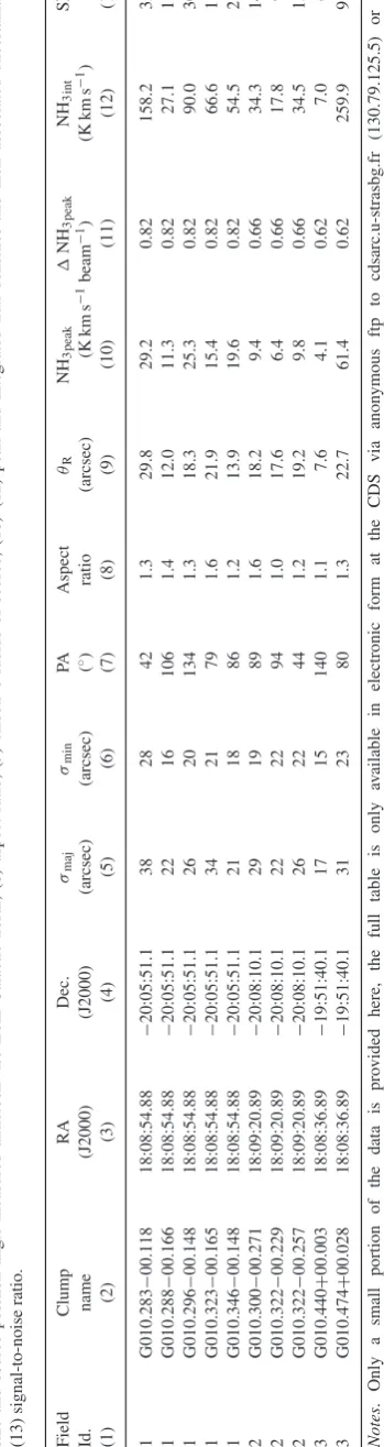
Ta b le 2 . The FellWalker source catalogue. T he parameters g iv en in this table ha v e been obtained from the higher signal-to-noise NH 3 (1,1) inte g rated emission maps. T he columns are as follo ws: (1) Field identification; (2) n ame d eri v ed from G alactic coordinates of the m aximum intensity in the source; (3)–(4) right ascension and d eclination in the J20 00 coordinate system; (5)–(7) semimajor and semiminor size and source position angle m easured anticlockwise from G alactic north; (8) aspect ratio; (9) ef fecti v e radius of source; (10)–(12) peak and inte grated flux d ensities and their associated uncertainties; (13) signal-to-noise ratio. Field Clump R A D ec. σmaj σmin P A Aspect θR NH 3 p eak NH 3 p eak NH 3i n t SNR Id. n ame (J2000) (J2000) (arcsec) (arcsec) ( ◦) ratio (arcsec) (K km s − 1beam − 1)( K k m s − 1) (1) (2) (3) (4) (5) (6) (7) (8) (9) (10) (11) (12) (13) 1 G 010.283 − 00.118 18:08:54.88 − 20:05:51.1 3 8 2 8 4 2 1 .3 29.8 29.2 0 .82 158.2 35.4 1 G 010.288 − 00.166 18:08:54.88 − 20:05:51.1 2 2 1 6 106 1.4 12.0 11.3 0 .82 2 7.1 13.7 1 G 010.296 − 00.148 18:08:54.88 − 20:05:51.1 2 6 2 0 134 1.3 18.3 25.3 0 .82 9 0.0 30.7 1 G 010.323 − 00.165 18:08:54.88 − 20:05:51.1 3 4 2 1 7 9 1 .6 21.9 15.4 0 .82 6 6.6 18.7 1 G 010.346 − 00.148 18:08:54.88 − 20:05:51.1 2 1 1 8 8 6 1 .2 13.9 19.6 0 .82 5 4.5 23.8 2 G 010.300 − 00.271 18:09:20.89 − 20:08:10.1 2 9 1 9 8 9 1 .6 18.2 9 .4 0.66 34.3 14.3 2 G 010.322 − 00.229 18:09:20.89 − 20:08:10.1 2 2 2 2 9 4 1 .0 17.6 6 .4 0.66 17.8 9.8 2 G 010.322 − 00.257 18:09:20.89 − 20:08:10.1 2 6 2 2 4 4 1 .2 19.2 9 .8 0.66 34.5 15.0 3 G 010.440 + 00.003 18:08:36.89 − 19:51:40.1 1 7 1 5 140 1.1 7 .6 4.1 0 .62 7 .0 6.6 3 G 010.474 + 00.028 18:08:36.89 − 19:51:40.1 3 1 2 3 8 0 1 .3 22.7 61.4 0 .62 259.9 98.9 Notes . O nly a small portion o f the data is pro v ided here, the full table is only av ailable in electronic form at the CDS v ia anon ymous ftp to cdsarc.u-strasbg. fr (130.79.125.5) or via http://cdsweb .u-strasbg.fr/cgi-bin/qcat?J/A + A/ .
[image:7.595.84.259.70.729.2]Figure 2. Cumulative distribution function of the aspect ratio of all of the clumps (i.e.σmaj/σmin).
Figure 3. Difference between the clump position angles and the Galactic mid-plane. The bin size is 10◦and the errors are estimated using Poisson statistics.
Figure 4. Cumulative distribution function of theY-factor of the clumps (i.e.Sν(int)/Sν(peak)).
at University of Leeds on March 30, 2016
http://mnras.oxfordjournals.org/
[image:7.595.309.547.519.705.2]Figure 5. Examples of the NH3 (1,1) and (2,2) spectra taken towards the position of the peak emission of the three clumps identified in the G010.315−00.251 field. The NH3(1,1) and (2,2) lines are shown as blue and green histograms, respectively, and the fits to these transitions are shown in red. Only a small portion of the data is provided here, the full fig-ure is only available in electronic form at the CDS via anonymous ftp to cdsarc.u-strasbg.fr (130.79.125.5) or via http://cdsweb.u-strasbg.fr/
cgi-bin/qcat?J/A+A/. Ta
b le 3 . Detected NH 3 clump parameters. The columns are as follo ws: (1) field ID gi v en in T able 1 ; (2) name deri v ed from G alactic coordinates of the p eak emission of each clump; (3)–(4) radial v elocity and the intrinsic F WHM line w idth; (5) optical depth o f the transition; (6)–(8) excitation, rotation and kinetic temperatures; (9) b eam filling factor ( Tex / Trot ); (10)–(11) NH 3 column density and ab undance. F o r columns (4)–(8) and (10)–(11), the first v alue is m easured to w ards the emission peak while the v alue g iv en in parentheses is the median v alue d etermined o v er th e clump. In the final column (12), w e include a fl ag to identify sources where b road line-widths are seen to w ards the centre o f clumps; a v alue o f 1 or 2 indicate whether the emission profile appears to arise from a single clump or multiple distinct clumps along the line o f sight, respecti v ely , and a v alue o f 3 identifies sources that are associated with broad emission wings, w hich are themselv es indicati v e of outfl o w motions. S ource names that are appended b y a † identifies clumps w ith w armer surf ace temperatures and colder centres (see Section 3 .4 for d etails). Field Clump vLSR v τmain Tex Trot Tkin Bff log( N (NH 3 )) log( N (NH 3 )/ N (H 2 )) Notes Id name (km s − 1)( k m s − 1)( K )( K )( K )( cm − 2)( cm − 2) (1) (2) (3) (4) (5) (6) (7) (8) (9) (10) (11) (12) 1 G 010.283 − 00.118 † 14.2 2 .4 (2.5) 4 .0 (3.4) 7 .0 (4.4) 17.0 (17.1) 18.8 (18.9) 0.26 15.35 (15.10) − 7.50 ( − 7.52) 1 G 010.288 − 00.166 † 12.2 1 .8 (1.9) 3 .9 (2.9) 4 .8 (4.1) 15.7 (16.3) 17.1 (17.9) 0.25 15.05 (14.96) − 7.45 ( − 7.35) 1 G 010.296 − 00.148 13.6 4 .2 (3.8) 1 .3 (1.6) 7 .6 (4.8) 21.2 (19.9) 24.6 (22.8) 0.24 15.22 (15.09) − 7.71 ( − 7.51) 2 G 010.300 − 00.271 29.1 4 .8 (3.5) 2 .3 (1.8) 3 .9 (4.0) 15.7 (15.5) 17.1 (16.8) 0.26 15.18 (14.90) − 7.35 ( − 7.32) 2 2 G 010.322 − 00.229 32.8 1 .9 (2.0) 3 .8 (3.3) 3 .9 (3.6) 14.9 (14.8) 16.1 (15.9) 0.24 14.98 (14.90) − 7.46 ( − 7.33) 2 G 010.322 − 00.257 32.8 2 .8 (2.5) 2 .8 (2.3) 4 .3 (3.9) 16.7 (16.1) 18.4 (17.7) 0.24 15.08 (14.88) − 7.66 ( − 7.40) 1 G 010.323 − 00.165 12.6 1 .7 (1.8) 3 .2 (2.8) 6 .2 (4.8) 18.3 (18.0) 20.6 (20.1) 0.27 15.08 (14.95) − 7.73 ( − 7.67) 1 G 010.346 − 00.148 † 12.2 1 .8 (2.0) 3 .2 (2.7) 6 .8 (5.3) 18.1 (18.9) 20.2 (21.3) 0.28 15.13 (15.01) − 7.50 ( − 7.64) 3 G 010.440 + 00.003 † 67.3 3 .7 (3.7) 1 .9 (1.9) 3 .6 (3.6) 14.9 (15.0) 16.1 (16.2) 0.24 14.94 (14.90) − 7.53 ( − 7.54) 3 G 010.474 + 00.028 67.2 5 .8 (4.1) 5 .6 (3.6) 5 .5 (4.0) 21.5 (18.2) 25.1 (20.4) 0.22 15.84 (15.32) − 7.75 ( − 7.25) 2 Notes . O nly a small portion o f the data is pro v ided here, the full table is only av ailable in electronic form at the CDS v ia anon ymous ftp to cdsarc.u-strasbg. fr (130.79.125.5) or via http://cdsweb .u-strasbg.fr/cgi-bin/qcat?J/MNRAS/ .
at University of Leeds on March 30, 2016
http://mnras.oxfordjournals.org/
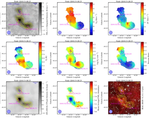
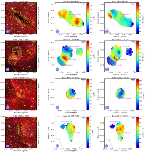
Figure 6. Distribution maps of the various parameters discussed in Section 2. In the upper-left panel, we present the integrated NH3 (1,1) emission map showing the area outlined in red in Fig.1. In the upper-middle and right-hand panels, we show the distribution of peak velocity and FWHM line width. The middle panels (left to right) show the kinetic temperature, ammonia column density, and gas pressure ratio (Rp; ratio of the squares of thermal and non-thermal line-widths), while in the lower panels we present the dust emission, ammonia abundance and the three-colour IRAC image. The contours are the same in every map, and trace the integrated NH3(1,1) emission as described in Fig.1. The magenta labels identify ammonia clumps identified byFellWalker, while the red triangles and blue crosses identify the positions of MYSOs and compact HIIregions identified by the RMS survey. The angular resolution of the GBT beam at this frequency is indicated by the blue hatched circle shown in the lower-left corner of each map. Only a small portion of the data is provided here, the full figure is only available in electronic form at the CDS via anonymous ftp to cdsarc.u-strasbg.fr (130.79.125.5) or viahttp://cdsweb.u-strasbg.fr/cgi-bin/qcat?J/A+A/.
have on the other derived properties. We estimate the non-thermal velocity using
vnt=
v2
int−
8ln2kBTkin
mNH3
. (4)
We have calculated values for the thermal and non-thermal linewidths for all pixels above the 3σ detection level in the inte-grated NH3(1,1) emission maps and used these to create ratio maps
showing the contribution of these components to the gas pressure ratio (Lada et al.2003);
Rp=
v2
th
v2 nt
, (5)
wherevthandvntare as previously defined. The pressure ratio
map is presented in the middle-right panel of Fig.6.
2.4 Beam filling factor
Ammonia emission is often found to be extended with respect to the beam; however, the excitation temperature of the inversion transi-tion is commonly found to be significantly lower than the estimated kinetic temperature of the gas, which suggests that the actual beam filling factor is less than unity (Bff=Tex/Trot∼0.1–0.3;Paper I;
Pillai et al.2006). There are two possible explanations for this: (1) the observed emission is the superposition of a large number of compact dense cores convolved with the telescope beam (i.e. there is structure on scales smaller than the beam); and (2) the gas is subthermally excited (i.e. non-LTE conditions). The latter is con-sidered less likely, however, as the densities are sufficiently high (>105cm−3; Keto, Caselli & Rawlings2015) for local
thermody-namical equilibrium (LTE) between the dust and gas.
The fitting algorithm calculates the kinetic and excitation tem-peratures. We calculate the rotation temperature from the derived
at University of Leeds on March 30, 2016
http://mnras.oxfordjournals.org/
kinetic temperature using the relationship (Walmsley & Ungerechts 1983)
Trot=Tkin/
1+Tkin
T0
ln1+0.6 exp (−15.7/Tkin)
. (6)
We have used these values to estimate the median and peak beam filling factors for the whole sample.8The peak filling factors are
similar to those derived inPaper I, although this study finds the median values are significantly lower (∼0.1), which would indicate that the more of the underlying substructure is concentrated towards the centre of the clumps. At the median distance of the sample, the beam size of ∼30 arcsec corresponds to a physical area of ∼0.4 pc2: this is several times larger than expected for a typical
core (r∼0.1 pc; e.g. Motte et al.2007) and it is therefore likely that the observed clump structures consist of multiple dense cores. This is consistent with recent higher resolution studies made with the VLA (e.g. Ragan et al.2011; Battersby et al.2014; Lu et al.2014).
2.5 Ammonia column density and abundance
The ammonia column density is determined as a free parameter by the fitting algorithm and uses the derived rotation temperature and so has therefore already taken the beam filling factor into ac-count. Determination of the column density assumes that excitation conditions are homogeneous and that all hyperfine lines have the same excitation temperature. The peak NH3column densities range
between 2.2 and 72.4×1014cm−2with a median value of 11.2×
1014cm−2. The column density in the outer envelope is significantly
lower, ranging between 2.2–19.1×1014cm−2with a median value
of 7.2×1014cm−2. The peak values for the NH
3column density
are consistent with studies reported towards other MSF regions and IRDCs that have been made at a similar resolution (e.g. Tafalla et al.
2004; Pillai et al.2006; Dunham et al.2011; Wienen et al.2012
and Morgan et al.2014). Although taking the beam filling factor into account produces more reliable peak NH3column densities
for the unresolved substructure, we note that when estimating the abundances using the dust emission it is in fact the beam-averaged column density that is of interest; this is because no correction is made for the substructure. The beam-averaged NH3column density
is therefore likely to be a factor of a few lower than that deter-mined by the algorithm. To compensate for this, we estimate the beam-averaged NH3column density by multiplying the maps by
the corresponding pixel beam filling factors.
To estimate the NH3 abundance, we compare the N(NH3) to
the totalN(H2) obtained from maps of the submm dust emission
extracted from the ATLASGAL (Schuller et al.2009) assuming a constant gas to dust ratio. ATLASGAL has surveyed the inner parts of the Galactic plane (300◦ < <60◦and |b| <1.5◦) at 870µm (345 GHz) where the dust emission is optically thin and is therefore an excellent probe of column density and the total mass of the clumps. Dust maps were extracted for all but two of the fields (G075.766+00.358 and G078.977+00.363 are located outside the ATLASGAL region). A Gaussian kernel with an FWHM of 25.6 arcsec was used to smooth the ATLASGAL maps to the same resolution as the GBT maps (i.e.(322−19.22)).
We use the kinetic gas temperature (Tkin) derived from the
ammo-nia emission for each pixel and the corresponding pixel flux from the ATLASGAL emission maps to create maps of the H2column
[image:10.595.306.542.53.241.2]8All peak measurements are taken towards the brightest NH3emission seen in the integrated maps presented in Fig1, which is nearly always found towards the centre of the clump.
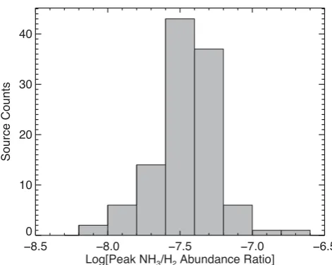
Figure 7. Frequency distribution of the peak NH3abundance relative to the H2within each clump obtained as in Section 2.5, for all clumps. The bin size is 0.2 dex.
density via
N(H2) = SνR
Bν(Tkin) κνμ mH,
(7)
where is the beam solid angle,μis the mean molecular weight of the ISM (we takeµ=2.8 assuming a 10 per cent contribution from helium; Kauffmann et al.2008),mH is the mass of the hydrogen
atom,Ris the gas-to-dust mass ratio (assumed to be 100) andκν
is the dust absorption coefficient (taken as 1.85 cm2g−1 derived
by Schuller et al.2009by interpolating to 870µm from Table1, column 5 of Ossenkopf & Henning1994). We are also assuming that the kinetic temperature is roughly equivalent to the dust temperature (i.e.Tkin=Tdust; e.g. Morgan et al.2010and Ko¨nig et al. 2015).
The H2and beam-averaged NH3column density maps have then
been combined to create maps showing variation in the ammonia abundance across the clumps (i.e.N(NH3)/N(H2)). For the
abun-dance analysis, we only include pixels where both the ammonia and dust emission is over 5σin order to minimize the uncertainty in the maps (lower-middle panel of Fig.6). From these maps, we estimate the fractional abundance in of the inner and outer envelopes and find these to be similar. The peak abundances range between 0.5 and 10.3×10⁻⁸with a median value of 2.5×10⁻⁸(see Fig.7
for the distribution). These values are consistent with many of the studies previously mentioned.
2.6 Uncertainties on the fitted parameters
FellWalkerdoes not provide estimates of the uncertainties for
the position or size of the extracted sources; we estimate that these values are likely to be accurate to within a few arcsec and so errors are relatively small given that most sources are well resolved. The uncertainty in the peak flux is determined from the standard de-viation of an emission-free region in each field, and is typically better than 10 per cent. We assume the uncertainty is similar for the integrated flux values.
The uncertainties in the velocity, line-width, optical depth, kinetic and excitation temperatures and NH3column density are estimated
by the fitting algorithm and are all relatively small. Typical uncer-tainties in the velocity and line-width are better than 0.1 km s−1and
0.3 K for kinetic and excitation temperatures, and since the rotation temperature is derived directly from the kinetic temperature it will
at University of Leeds on March 30, 2016
http://mnras.oxfordjournals.org/
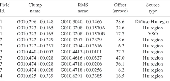
Table 4. RMS associations.
Field Clump RMS Offset Source
Id. name name (arcsec) type
1 G010.296−00.148 G010.3040−00.1466 28.6 Diffuse HIIregion 1 G010.323−00.165 G010.3208−00.1570A 32.6 HIIregion 1 G010.323−00.165 G010.3208−00.1570B 17.7 YSO 2 G010.322−00.229 G010.3207−00.2329 8.6 HIIregion 2 G010.322−00.257 G010.3204−00.2616 6.2 HIIregion 3 G010.440+00.003 G010.4413+00.0101 27.7 HIIregion 3 G010.474+00.028 G010.4616+00.0327 47.0 HIIregion 3 G010.474+00.028 G010.4718+00.0206 36.1 HIIregion 3 G010.474+00.028 G010.4718+00.0256 6.2 HIIregion 4 G010.625−00.339 G010.6291−00.3385 16.5 HIIregion Notes:Only a small portion of the data is provided here, the full table is only available in electronic form at the CDS via anonymous ftp to cdsarc.u-strasbg.fr (130.79.125.5) or viahttp://cdsweb.u-strasbg.fr/cgi-bin/qcat?J/A+A/.
have a similar uncertainty. The uncertainty for the beam filling factor will be dominated by the uncertainty in the excitation temperature, which is roughly about 5 per cent. Although the uncertainty in the NH3column density given by the code is small, it is dominated by
the uncertainty in the peak flux measurement, which as mentioned in the previous paragraph is∼10 per cent and we therefore adopt this value for the uncertainty for this parameter. Finally, we estimate the uncertainty in the abundance ratio to be∼20 per cent, which is a combination of the uncertainty in the peak fluxes of the ATLAS-GAL survey (∼15 per cent; Schuller et al.2009) and NH3added in
quadrature; however, this is a lower limit as the dust models used to estimate the H2column densities are not well constrained and so
the true uncertainty can be a factor of a few times the abundance.
3 R E S U LT S
3.1 Detection statistics
We have detected a total of 115 clumps in the 66 fields observed as part of this project. Integrated NH3(1,1) maps of all of the observed
fields are presented in Fig. A1 and all of the clump parameters determined byFellWalkerare given in Table2.
In Fig.6, we present distribution maps of field G010.31−00.25 produced from the analysis described in the previous section. 31 of the 115 clumps identified have peak integrated NH3(1,1) emission
below an SNR value of 10, which is too low to allow detailed anal-ysis of the spatial distribution of the various parameters derived, particularly those that also rely on the detection of the (2,2) tran-sition. The peak and median values for the derived properties for these lower SNR clumps are given in the results tables, although we do not explicitly present the spatial distribution maps of these low-SNR clumps or discuss them in detail. Distribution maps are provided in Fig A6 of all 84 clumps with an SNR of 10 of more.
3.2 RMS associations
We have matched these clumps with the RMS catalogue to dis-tinguish those associated with massive star formation from those likely to be less active (quiescent). A match was made between a clump and an RMS source if the RMS source was located within clump boundaries as defined by the lowest contour shown in Fig.1 (i.e. 3σ) and possessed a similarvLSRas the clump. In 21 cases,
multiple RMS sources have been associated with the same clump. We find 71 clumps are associated with RMS sources while the star
Figure 8. Distribution of the surface density of sources with a given angular separation between the peak emission from the clump and the nearest RMS association. The bin size is 5 arcsec.
formation is less evolved towards the remaining 44 clumps (approx-imately 40 per cent of the clumps identified); here, we are making the assumption that infrared faint/dark clumps are less evolved. We therefore have a useful sample of relatively quiescent clumps (i.e. not currently associated with an MYSO or HIIregion) with which
to compare the results from our more evolved sample. We also find there is no difference in the proportions of RMS sources associated with spherical and filamentary clumps.
In Table4, we present a list of RMS and clump associations, the RMS classification, and the angular separation between the peak emission position of the ammonia and the position of the embedded HIIregion or MYSO. In Fig.8, we show the distribution
of angular separations between the embedded RMS sources and the peak of the integrated NH3(1,1) emission. This plot reveals a strong
positional correlation between the embedded massive stars and the peak ammonia emission seen towards the centre of the clumps, with the vast majority of embedded objects having offsets of less than 10 arcsec. We find no significant difference in the separations between the MYSOs and the HII regions. The star formation is
therefore primarily taking place towards the centres of centrally condensed clumps where the column densities are highest.
at University of Leeds on March 30, 2016
http://mnras.oxfordjournals.org/
[image:11.595.309.547.254.448.2]We note that the peak of the offset distribution is shifted from zero, with the embedded sources typically found between 5–10 arcsec from the ammonia emission peak. This is larger than the nominal pointing error (∼4 arcsec) and is a little surprising given that a tighter correlation between the embedded sources and the peak of the dust emission has been previously observed (i.e. Urquhart et al. 2014a,c). A similar angular offset was recently reported by Morgan et al. (2014) from a comparison of the dust and ammonia emission peaks from clumps associated with the Perseus molecular cloud. These authors suggested that these two tracers may be sensitive to different conditions or structure in the clumps. In many cases, the ammonia emission is clearly much more extended than the dust emission (e.g. G011.918−00.618 and G014.328−00.646), which would support this hypothesis. Another possibility is that feedback from the embedded massive stars is starting to alter the structure and composition of their local environments, resulting in a shift in position of the peak column density away from the massive stars (Thompson et al.2006).
Although the offset between the peak of the ammonia emission and the embedded source is significantly larger than that found between the embedded source and the dust emission, the difference is only a fraction of the GBT beam and so is relatively small. Furthermore, although the angular offset is noticeable we will see in Section 3.5 that the actual physical offset is less obvious once the distance to the source has been taken into account.
3.3 Mid-infrared imaging
To investigate the embedded protostellar population and evaluate the influence of the local environment, we have extracted mid-infrared
images from the GLIMPSE legacy survey (Benjamin et al.2003; Churchwell et al.2009). We combined the 3.5, 4.5 and 8µm band images obtained with the IRAC instrument (Fazio et al.2004) to produce three-colour images of the mid-infrared environment.
These images are very sensitive to embedded objects such as MYSOs and compact HII regions, and provide a census of the
embedded stellar content of these clumps (see lower-right panel of
Fig.6). Extinction results in a greater reddening for the more deeply
embedded objects in these three-colour images. As a result, these images not only reveal the stellar content and their luminosity but also provide hints to their evolutionary stage.
The 8µm band is sensitive to emission from polycyclic aromatic hydrocarbons (PAHs) that are excited by UV-radiation from em-bedded compact HIIregions as well as large nearby HIIregions,
and thus is an excellent tracer of the interaction regions between ionized and molecular gas. The 4.5µm band includes excited H2
and CO transitions which are thought to trace shocked gas driven by powerful molecular outflows. Excess emission seen in this band is therefore considered a good tracer of massive star formation (e.g. Cyganowski et al.2008,2009). These images can therefore be useful to understand some of the temperature and velocity structure observed in the clumps with respect to the position of the embedded MYSOs and HIIregions.
3.4 General properties of the sample
[image:12.595.61.533.415.739.2]The statistics for the parameters derived in the previous section for the whole sample are given in Table5along with bolometric luminosities taken from the RMS survey; where the median and peak values are significantly different we provide both values.
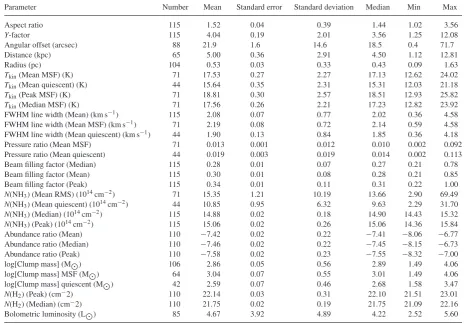
Table 5. Statistical properties for the whole sample.
Parameter Number Mean Standard error Standard deviation Median Min Max
Aspect ratio 115 1.52 0.04 0.39 1.44 1.02 3.56
Y-factor 115 4.04 0.19 2.01 3.56 1.25 12.08
Angular offset (arcsec) 88 21.9 1.6 14.6 18.5 0.4 71.7
Distance (kpc) 65 5.00 0.36 2.91 4.50 1.12 12.81
Radius (pc) 104 0.53 0.03 0.33 0.43 0.09 1.63
Tkin(Mean MSF) (K) 71 17.53 0.27 2.27 17.13 12.62 24.02
Tkin(Mean quiescent) (K) 44 15.64 0.35 2.31 15.31 12.03 21.18
Tkin(Peak MSF) (K) 71 18.81 0.30 2.57 18.51 12.93 25.82
Tkin(Median MSF) (K) 71 17.56 0.26 2.21 17.23 12.82 23.92
FWHM line width (Mean) (km s−1) 115 2.08 0.07 0.77 2.02 0.36 4.58
FWHM line width (Mean MSF) (km s−1) 71 2.19 0.08 0.72 2.14 0.59 4.58
FWHM line width (Mean quiescent) (km s−1) 44 1.90 0.13 0.84 1.85 0.36 4.18
Pressure ratio (Mean MSF) 71 0.013 0.001 0.012 0.010 0.002 0.092
Pressure ratio (Mean quiescent) 44 0.019 0.003 0.019 0.014 0.002 0.113
Beam filling factor (Median) 115 0.28 0.01 0.07 0.27 0.21 0.78
Beam filling factor (Mean) 115 0.30 0.01 0.08 0.28 0.21 0.85
Beam filling factor (Peak) 115 0.34 0.01 0.11 0.31 0.22 1.00
N(NH3) (Mean RMS) (1014cm−2) 71 15.35 1.21 10.19 13.66 2.90 69.49
N(NH3) (Mean quiescent) (1014cm−2) 44 10.85 0.95 6.32 9.63 2.29 31.70
N(NH3) (Median) (1014cm−2) 115 14.88 0.02 0.18 14.90 14.43 15.32
N(NH3) (Peak) (1014cm−2) 115 15.06 0.02 0.26 15.06 14.36 15.84
Abundance ratio (Mean) 110 −7.42 0.02 0.22 −7.41 −8.06 −6.77
Abundance ratio (Median) 110 −7.46 0.02 0.22 −7.45 −8.15 −6.73
Abundance ratio (Peak) 110 −7.58 0.02 0.23 −7.55 −8.32 −7.00
log[Clump mass] (M) 106 2.86 0.05 0.56 2.89 1.49 4.06
log[Clump mass] MSF (M) 64 3.04 0.07 0.55 3.01 1.49 4.06
log[Clump mass] quiescent (M) 42 2.59 0.07 0.46 2.68 1.58 3.47
N(H2) (Peak) (cm−2) 110 22.14 0.03 0.31 22.10 21.51 23.01
N(H2) (Median) (cm−2) 110 21.75 0.02 0.19 21.75 21.09 22.16
Bolometric luminosity (L) 85 4.67 3.92 4.89 4.22 2.52 5.60
at University of Leeds on March 30, 2016
http://mnras.oxfordjournals.org/
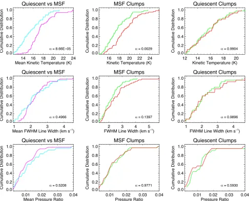
Figure 9. Left-hand panels: cumulative distribution plots comparing the mean values for the kinetic temperature, FWHM line width and pressure ratio for the MSF and quiescent clumps (cyan and magenta curves, respectively). Middle and right-hand panels: cumulative distribution plots comparing the peak and median values (shown in red and green, respectively) for the MSF and quiescent clumps for the same parameters. These allow us to identify any significant differences between the internal and external structure of the clumps. The results of KS tests comparing the peak and median values is given in the lower-right corner of each plot. For these plots and the discussion in the text, we only include sources with an SNR>10.
Nearly all of the clumps are extended with respect to the beam and have a relatively simple morphology with their emission distribution being reasonably well described by an ellipse with aspect ratio ∼1.5. The internal structures and dynamics of the gas of many of the clumps, however, are complicated and hard to interpret. This is made more difficult by the external environment that is heating the surface layers of the clumps and affecting the kinematics. As noted by Ragan et al. (2011), a single model is unlikely to account for the large range of properties observed; however, in this section we attempt to give an overview of the general properties of the clumps and will endeavour to provide a more detailed discussion of some of more interesting differences in later sections.
We find a correlation between the position angles of the clumps and the Galactic plane, such that the semimajor axis of the clumps are preferentially aligned parallel to the Galactic mid-plane (see
Fig.3). Furthermore, examination of the velocity information
re-veals typical velocity gradients of a couple of km s−1and these tend
to also be aligned along the semimajor axis. There are relatively
few examples of clumps that show no sign of a velocity gradient (e.g. G022.412+00.316).
We present in Fig.9the cumulative distribution plots comparing the median and peak values for the kinetic temperature, FWHM line width, and the gas pressure ratio (Rp) for the whole sample
and the MSF and quiescent subsamples. We use the peak and median values of these parameters to compare the conditions to-wards the centres of the clumps with their outer envelopes, and refer to these as ‘inner’ and ‘outer envelope’ values, respectively. In the lower-right corner of these plots, we give the results of Kolmogorov–Smirnov (KS) tests, α, which is the probability of the two samples being drawn from the same population. In order to reject the null hypothesis that any two distributions are drawn from the same parent distribution with greater than 3σconfidence, the value ofαmust be lower than 0.0013. In Fig.10, we present the mid-infrared image and temperature and line width distribution maps for a selection of clumps to help illustrate some of the features discussed in the following paragraphs.
at University of Leeds on March 30, 2016
http://mnras.oxfordjournals.org/
Figure 10. Three-colour mid-infrared images and distribution maps of the kinetic temperature and line width for a range of clump types. The contours are the same in every map and trace the integrated NH3(1,1) emission as described in Fig.1while the symbols used and labels are as described in Fig.6. In the upper, upper-middle, lower-middle and lower panels, respectively, we present examples of: a quiescent clump showing a relatively smooth temperature and velocity distribution; an example of a clump associated with an RMS source that is coincident with a localized increase in both the line-width and temperature, which is indicative of feedback from the embedded HIIregion; a clump located in the edge of a HIIregion, which is having an impact on the exposed side of the clump; and a clump associated with MYSOs that is coincident with a localized enhancement of the line-widths, which may be linked to the molecular outflow.
Comparison of the MSF and quiescent distributions for these three parameters reveals that the only significant difference between them is their kinetic temperatures, which are clearly higher for the MSF clumps.
Inspection of the kinetic temperature and line width cumula-tive distribution plots (Fig.9) for the quiescent clumps indicates that there is no significant difference between the inner and outer envelopes of these sources. This is also seen in the example
distribution map presented in the upper panel of Fig. 10, where the quiescent clump displays a relatively flat distribution for these parameters. This is consistent with the interpretation that these clumps are in a more homogeneous (‘pristine’) state prior to the onset of star formation. The distributions of these two parameters are very different for the MSF clumps where the internal tempera-tures and line widths are clearly seen to be higher than in the outer envelope.
at University of Leeds on March 30, 2016
http://mnras.oxfordjournals.org/
A temperature gradient is clearly seen in many of the distribu-tion maps presented in Fig.6, with the peaks often coincident with the positions of the embedded infrared sources seen in the IRAC images (see also Fig.10). The peak temperatures are∼20 K and decrease to∼12 K towards the edges of the clumps. This suggests that feedback from the central object is having a significant impact on the temperature and dynamics of the surrounding gas. The KS test confirms that the temperature difference between the inner and outer envelope is statistically significant. Furthermore, the temper-ature distributions within the MSF clumps display sharper spatial variation and more complex distribution patterns, which is possibly evidence of feedback from the embedded massive stars.
Comparison of the temperature distribution maps reveals a subsample of 34 clumps where the outer envelope is higher than found towards the central region (e.g. G012.887+00.492, G013.332−00.039 and G019.080−00.290; all of these are iden-tified in Table3). The majority of these (21) are members of the quiescent sample, but approximately one-third (13) are members of the MSF sample. A negative temperature gradient is not unexpected for the quiescent clumps because their exteriors are exposed to the interstellar radiation field while their inner regions are shielded (e.g. Wang et al.2008; Peretto et al.2010), but is perhaps a little surpris-ing for the MSF clumps. Examination of the mid-infrared images reveals that many are located near the periphery of large HIIregions where the strong radiation fields and expanding ionization fronts are clearly having an impact on their temperature and velocity structure (see lower-middle panels of Fig.10for an example).
The observed line widths are more complex than a simple ra-dial profile expected from a single velocity component. There is evidence of an increase in the line width towards the centres of approximately two-thirds of the clumps (a note in Table3identifies these sources and provided an indication of their nature). In total, 54 clumps are associated with significantly higher velocity disper-sions towards their centres with the majority being associated with massive star formation (40). For the MSF clumps, the broadest line widths are not only coincident with the peak of the integrated NH3
emission but also closely correlated with the position of the embed-ded source. A KS test does not find a significant difference between the line widths of the inner and outer envelopes of the MSF clumps. This may be due to the small sample size and because the line pro-files can result from the blended emission from multiple clumps and can include infall and outflow motions, making the interpretation of the distribution maps difficult in some cases.
Inspection of the line profiles reveals evidence for the presence of multiple components towards∼23 per cent of the clumps (19/82), with the emission profile seen towards∼40 per cent appearing to be consistent with a single source (34/82), while one source is classified as ambiguous (G045.467+00.046). 11 clumps show evidence of line wings, which are usually indicative of the presence of molecular outflows. The remaining clumps (24 per cent of the sample) show no significant increase in their line widths towards the centre of the clumps. In Fig.11, we show an example of the three types of profiles discussed.
[image:15.595.311.546.55.669.2]The problem of multiple components is a difficult one to deal with as often the velocity components are blended and cannot be separated in a reliable way. Caution should be exercised when inter-preting the line width, temperature and column density distributions in these cases, as these quantities have been derived from a single fit to blended profile and therefore the peak values may be a little less reliable, however, the mean values should not be significantly affected. This is only likely to affect∼20 per cent of the sample and so is unlikely to impact the statistical results; however, it is
Figure 11. Examples of NH3spectra towards regions of high-velocity dis-persion. The upper, middle and lower panels present an example of single component (40 per cent), multiple component (23 per cent) and wing com-ponent (13 per cent) profiles, respectively. The NH3 (1,1) and (2,2) lines are shown as blue and green histograms, respectively, and the fits to these transitions are shown in red.
at University of Leeds on March 30, 2016
http://mnras.oxfordjournals.org/